Clean Answers over Dirty Databases: A ... - University of Toronto

Clean Answers over Dirty Databases: A Probabilistic Approach Periklis Andritsos University of Trento [email protected]

Ariel Fuxman University of Toronto [email protected]

Abstract The detection of duplicate tuples, corresponding to the same real-world entity, is an important task in data integration and cleaning. While many techniques exist to identify such tuples, the merging or elimination of duplicates can be a difficult task that relies on ad-hoc and often manual solutions. We propose a complementary approach that permits declarative query answering over duplicated data, where each duplicate is associated with a probability of being in the clean database. We rewrite queries over a database containing duplicates to return each answer with the probability that the answer is in the clean database. Our rewritten queries are sensitive to the semantics of duplication and help a user understand which query answers are most likely to be present in the clean database. The semantics that we adopt is independent of the way the probabilities are produced, but is able to effectively exploit them during query answering. In the absence of external knowledge that associates each database tuple with a probability, we offer a technique, based on tuple summaries, that automates this task. We experimentally study the performance of our rewritten queries. Our studies show that the rewriting does not introduce a significant overhead in query execution time. This work is done in the context of the ConQuer project at the University of Toronto, which focuses on the efficient management of inconsistent and dirty databases.

1 Introduction The detection of duplicate records that correspond to the same real-world entity is an important task in data integration and data cleaning. Duplicates may occur due to data entry errors or to the integration of data from disparate sources. Many techniques exist for detecting duplicate records [1, 6, 13, 15, 16, 18, 19, 20]. These techniques may be based on clustering, classification, or other link-analysis or statistical techniques. Duplicate detection is sometimes called tuple matching and is supported by commercial data integration tools such as IBM WebSphere QualityStage1 and FirstLogic Information Quality2 . Partially supported by NSERC. 1 http://www.ascential.com/products/qualitystage.html 2 http://www.firstlogic.com/dataquality/

Ren´ee J. Miller University of Toronto [email protected]

Even in carefully integrated databases where structural and semantic heterogeneity has been resolved, duplication may occur due to true disagreement among the sources. That is, two data sources may record different (inconsistent) information about the same entity. This is a common situation, for example, in the domain of Customer Relationship Management (CRM). One of the goals of CRM is to produce an integrated database from a variety of sources containing customer data. It is often the case that the sources contain conflicting information about the same customer. Commercial data integration tools typically use conflict resolution rules to support the merging of tuples corresponding to the same entity. Examples include rules that take the average between multiple conflicting incomes of the same customer. Such rules (sometimes called survivorship rules) may be hard to design, particularly for categorical data where values cannot always be combined. Furthermore, for some applications, there may be no set of rules that correctly resolve all current and future conflicts. In the absence of complete conflict resolution rules, some data integration tools keep conflicting tuples in the integrated database. In this work, we consider the problem of query answering over dirty databases. Typically, existing data integration tools assume that queries can be executed directly on the dirty database. However, this fails to address the semantics of duplication. For example, suppose that a customer called John has two (inconsistent) incomes of $80K and $120K in the dirty database. Assume that we want to answer the query “get customers who make more than $100K a year”. Using standard query answering, John would appear in the answer. However, our intuition is that we do not know with high certainty whether John is in the answer because according to one of the sources his income may be $80K. The first question that we address here is: what is a good semantics for querying dirty databases? To this end, we note that duplicate tuples are alternative representations for the same real-world entity. In a clean database, only one representation will be present for each entity. In the absence of additional information (such as conflict resolution rules), we will assume that the representation in the clean database includes values from the duplicates. Hence, a dirty database

represents several possible databases that are candidates to be in the clean database. If each real-world entity is assigned a unique key, we can think of the dirty database as an inconsistent database that violates a set of key constraints [4]. We adopt a probabilistic semantics for querying dirty databases. For this, it is necessary to associate probabilities to each of the tuples of the inconsistent database. There are different ways for assigning such probabilities. For example, we could assign probabilities to the sources: the more reliable the source, the higher its probability. Then, we could use provenance information to assign probabilities to the tuples in the integrated database taking their origin into account. In the absence of provenance information, we could just assume uniform probabilities. Finally, the probabilities may be the output of a tuple matching process performed by a data integration tool. In this paper, we present a new semantics for querying duplicated data using a notion that we call clean answers. The semantics of clean answers is independent of the way the probabilities are produced, but is able to effectively exploit them during query answering. In particular, each answer is given together with its probability of being in the clean database. loyaltyCard cardId custFk prob 111 c1 0.4 111 c2 0.6

customer custId name c1 John c1 John c2 Mary c2 Marion

income $120K $80K $140K $40K

income is below $100K. In the semantics of clean answers, we consider all possible databases that can be obtained from the dirty database by choosing exactly one tuple for each duplicate. There are eight possible databases in this example. Each possible database can be assigned a probability. For examfor card 111, and tuples and ple, if we choose tuple for John and Mary, respectively, we obtain a possible database . Since the tuples for each duplicate are chosen independently from the other duplicates, the probability of the possible database is obtained by multiplying the probabilities of its tuples. For , we get a probability of . The clean answer is obtained by summing the probabilities of all possible databases that satisfy the query. In this case, card 111 is in the result of applying the query to four out of the eight possible databases: . Their probabilities are , and 0.024, respectively. Since the sum of these probabilities is 0.6, we will say that card 111 has 60% of probability of being associated with a customer earning over $100K.pp The semantics of clean answers is based on proposals for probabilistic databases [5, 9, 12, 17]. In probabilistic query answering, a set of answers is computed together with their probability of being correct. A distinctive feature of our approach is that it uses an SQL query rewriting, that is, given a query, we rewrite it into another SQL query that produces an answer together with the probability of the answer being in the clean database. While the semantics of probabilistic databases has been well explored, to the best of our knowledge, Dalvi and Suciu [12] are the first to consider query rewriting for probabilistic databases. They consider a semantics in which tuple probabilities are independent. For independent tuples, in any possible database, the probability of one tuple being in the clean database is independent of any other tuple. We cannot make this assumption for duplicated data. Recall that our possible worlds represent potential clean databases which contain exactly one tuple for each real-world entity. Hence, given a group of potential duplicates containing tuples and , if is in a possible database, then the probability of being in that database is zero. Hence, and are not independent. We address this by proposing a new semantics under which tuples representing the same entity are conditionally dependent, and tuples representing different entities are independent. This work is done in the context of the ConQuer project at the University of Toronto.3 This project focuses on the efficient management of inconsistent and dirty databases. In this paper, we make the following contributions.

prob 0.9 0.1 0.4 0.6

Figure 1. A dirty customer database. We now illustrate the semantics of clean answers through an example. In Figure 1, we show a dirty database with information regarding a customer loyalty program. There are two tables: loyaltyCard, which associates card numbers to customers; and customer which stores customers and their income. The attributes cardId and custId represent identifiers, where tuples sharing the same identifier have been determined to be duplicates. The attribute custFk of the loyaltyCard relation is a foreign key to the customer relation. Finally, each tuple has a probability (indicated in attribute prob) representing the likelihood of the tuple being in the clean database. Suppose that we want to get the card numbers of customers who have an income above $100K. Intuitively, card 111 should be in the answer because there is some evidence that it belongs to John, who has an income above $100K with a very high probability. One might ask if it suffices to just clean the database off-line and then answer the query. For example, we may want to remove all the tuples for each duplicate except the one with the highest probability. In this case, we would remove , and . But then, the result of the query is empty because tuple (the only tuple for card 111) joins only with tuple , representing Marion whose

We propose a new semantics for querying duplicated data. This semantics complements and extends previous proposals 3 ConQuer

2

stands for Consistent Querying

in the areas of probabilistic databases and consistent query answering. We propose a query rewriting technique that, for a large class of select-project-join queries, rewrites the query into an SQL query that computes the answers to the query and their probabilities according to the semantics that we define for dirty databases. We show that although a rewriting cannot be obtained in general, the rewriting that we propose here works for many queries that arise in practice.

determined to correspond to the same real-world entity as a cluster. Dfn 1 (clustering) Let be a relation. A clustering partitions into disjoint sets of tuples , called clusters, such that . Most tuple matching techniques apply to a single table; others use information from multiple tables to detect potential duplicates [6]. However, this distinction is immaterial to our discussion. We only require that the final output of the technique be a clustering on each dirty relation. Matching techniques output cluster identifiers, though the way these identifiers are modeled may differ between tools. For example, some tools, like WebSphere QualityStage, output cross-reference tables that indicate which tuples are associated with which cluster. To use the clustering information in query answering, we will assume that each table has an identifier attribute containing the cluster identifer. This identifier attribute (again depending on the matching tool) may be added to the table as a new column. Alternatively, some matchers will choose one of the key values from the tuples in a cluster to be the identifier for the cluster. Each tuple in the cluster is then assigned this same key value. In this latter approach, the original key attribute of the table will contain the cluster identifier. In either case, the identifier attribute will contain duplicate values (and hence will not be a key of the relation). Regardless of which approach is used by the tuple matching tool, the foreign keys of all relations must be updated to refer to the identifiers. This is a simple process, which we will call identifier propagation, that is supported by many matching tools. Finally, we assume that each tuple is assigned a probability, in such a way that there is a probability function for each cluster. By definition of probability function, the sum of the probabilities of all tuples within a cluster must be 1. Clearly, a clean tuple (that is, a tuple with no other matching tuples) will have a probability of 1.

We propose a method that uses the output of a tuple matching technique to assign probabilities to potential duplicates. Our method can be used with tuple matching techniques that only produce groupings of duplicates (with no additional information), or with techniques that output groupings together with a similarity measure or the distance between duplicates [3, 6, 16, 18, 19, 20]. Our method has the advantage that it performs well on categorical data values. It is beyond the scope of this paper to compare the relative advantages of different tuple matching techniques including ours. Deduplication is a well studied area and different approaches are known to work well for different applications and data characteristics. One of the benefits of our approach is that it is modular and can work with different techniques that find matching tuples. Using real data, we argue that the computed probabilities have an intuitive semantics and can be computed efficiently. We also show that our rewritten queries can be executed efficiently on large databases. Our studies show that the rewriting does not introduce a significant overhead in the execution time over the original query. The paper is organized as follows. In Section 2, we define dirty databases and the semantics of clean answers. In Section 3, we present a rewriting that given a query, computes another query that retrieves the clean answers. In Section 4, we present a technique for assigning probabilities to duplicates in a dirty database. Section 5 presents the efficiency evaluation of our approach and, finally, Section 6 concludes the paper and discusses future challenges.

Dfn 2 (dirty database) A dirty database is a database and a where for each relation , we have a clustering function that maps the tuples of to a probability value. The probabilities within each cluster must sum to 1.

2 Dirty Databases and Clean Answers We begin this section by discussing how we model dirty databases. Then, we present our semantics for query answering over such databases.

2.1 Dirty Databases

The following example illustrates how a database with duplicates can be modeled as a dirty database that we can use for query answering.

We assume that the dirty databases we use for query answering have been pre-processed by some data integration tool. The first pre-processing step is tuple matching. The output of a matching technique is a grouping or clustering of tuples. We will refer to a group of tuples that have been

Example 1 Consider the database of Figure 2. This database consists of two dirty tables, order and customer with original schema order[orderId,custFk,quantity] and customer[custId,name,balance], respectively. We 3

order

id o1 o2 o2

orderId 11 12 13

custFk m1 m2 m3

cIdFk c1 c1 c2

quantity 3 2 5

customer

prob 1 0.5 0.5

id c1 c1 c2 c2

custId m1 m2 m3 m4

name John John Mary Marion

balance $20K $30K $27K $5K

prob 0.7 0.3 0.2 0.8

Figure 2. A dirty database with order and customer relations have introduced two new attributes into the customer relation, id and prob, for the identifier the tuple matcher produces and for the tuple probabilities. In relation order, we introduce these same two attributes, but in addition, we introduce a new attribute cIdFk for the identifier of the customer referenced by order.custFk. The values of attribute cIdFk are updated using identifier propagation.

according to their semantics), and therefore cannot be used for our purposes. Example 2 Consider the dirty customer and order relations from Figure 2. There are eight candidate databases:

2.2 Clean Answers

Clearly, not all candidate databases are equally likely to be clean. We model this with a probability distribution, which assigns to each candidate database a probability of being clean. Since the number of candidate databases may be huge (exponential in the worst case), we do not give the distribution by extension. Instead, we use the probabilities of each tuple (function ) to calculate the probability of a candidate database being the clean database. Since tuples are chosen independently from each cluster, the probability of each candidate database can be obtained as the product of the probability of each of its tuples.

It is well known how to answer queries over clean databases. But, how can we answer queries over a dirty database? And, what is the interpretation of the query results? One alternative is to return an answer together with its probability of being obtained from the clean database. In order to do this, one needs a clear indication of which databases may be clean. In our framework, this indication can be obtained from the semantics of duplication. In particular, since the clean database has no duplicates it is reasonable to assume that it consists of exactly one tuple from each cluster of the dirty database. The following is our definition of a candidate database.

Dfn 4 (probability distribution over candidates) Let be a dirty database. The probability of a candidate database is defined as:

Dfn 3 (candidate database) Let be a dirty database. We say that is a candidate database for if (1) is a subset of ; and (2) for every cluster of a relation in , there is exactly one tuple from such that is in .

Notice that, in contrast to the definitions given for cases where tuple independence is assumed [12], we do not need to consider tuples that are not in the candidate database. The reason is that, since every candidate has exactly one tuple from each cluster, the probability of such a tuple not being in the candidate is 1.

Candidate databases are related to the notion of possible worlds, which has been used to give semantics to probabilistic databases [12]. Notice, however, that the definition of candidate database imposes specific conditions on the tuple probabilities. First, the tuples within a cluster must be exclusive events (a very strong form of conditional dependence), in the sense that exactly one tuple of each cluster appears in the clean database. Second, the probabilities of tuples from different clusters are independent. Cavallo and Pittarelli [9] proposed a model in which all the tuples in a relation are assumed to be exclusive events. In our terms, they assume that each relation consists of exactly one cluster. At the other extreme, most work on probabilistic databases assumes that tuple probabilities are independent [14, 5, 12]. To the best of our knowledge, the only work that considers conditional probabilities in a way that satisfies our conditions is ProbView [17]. However, their work does not focus on producing a rewritten query (i.e., a query that computes the answer

Example 3 The following are the probabilities for each of the candidate databases for the dirty database of Figure 2.

We are now ready to give the semantics of query answering in our framework. Recall that the clean database is unknown. However, we can still reason about the answers obtained by applying the query to the candidate databases. Intuitively, a result is more likely to be in the answer if it is obtained from candidates with higher probability of being clean. Therefore, for each tuple of the query result, we will consider the candidates from which it can be obtained, and sum their probabilities. 4

0.07 0.28 0.03 0.12 0.07 0.28 0.03 0.12

Dfn 5 (clean answer) Let be a dirty database. We say that a tuple is a clean answer to a query if there exists a candidate database such that . The probability of is: Example 4 Consider a query that retrieves all the customers whose balance is greater than $10K. select id from customer c where balance > $10K

Figure 3. Candidates for database of Figure 2

( )

queries in this class, there is a simple query rewriting that computes the clean answers directly from the dirty database. We start with a number of motivating examples before introducing the rewriting algorithm.

Customer has a balance greater than $10K in every candidate. Thus, it is a clean answer with probability 1. Customer satisfies the query only in candidates and , and . Therefore, is a clean answer with a probability of .20.

Example 5 Consider again the query that retrieves the customers with a balance greater than $10K. We showed in Example 4 of the previous section that the clean answer for this query on the dirty database of Figure 2 is . Consider a na¨ıve rewriting that returns the probability associated with each tuple.

The notion of clean answers is a generalization of the consistent answers that were defined by Arenas et al. [4] in the context of query answering over inconsistent databases. In particular, if each tuple of the dirty database is assigned a non-zero probability of being in the clean database, then the consistent answers of a query correspond to the clean answers that have a probability of 1 (that is, complete certainty).

select id, prob from customer c where balance > $10K

The result of applying this rewritten query to the dirty , which is not the database is clean answer. However, we can obtain the clean answer anand summing their swer by grouping the two tuples for probabilities. Therefore, the following query returns the clean answers for .

3 Efficient Computation of Clean Answers The clean answers to a query can be obtained directly from the definition if we assume that all the candidate databases of a given dirty database are available. But this is an unrealistic assumption because, in the worst case, the number of candidate databases may be exponential in the size of the dirty database. Since our goal is the efficient computation of clean answers, we present techniques that avoid the materialization of the candidate databases altogether. In particular, we use an approach based on query rewriting. That is, given a query , we produce another query that can be applied directly on any dirty database in order to obtain the clean answers and their probabilities for . There are some queries for which there is no SQL rewriting that computes the clean answers. This follows from existing results in the literature for the problem of obtaining consistent answers which, as we explained in the previous section, is a special case of clean answers. In particular, it has been shown that there are some Select-Project-Join (SPJ) queries for which the problem of obtaining consistent answers is co-NP complete [8, 10]. This implies that, unless P=NP, there are some SPJ queries for which there is no SQL rewriting that computes the clean answers. Thus, the question is: are there large and practical classes of queries for which the clean answers can be efficiently computed? We will show in this section that the answer to this question is positive. More importantly, we will show that, for the

select id, sum(prob) from customer c where balance > $10K group by id

The previous example focuses on a query with just one relation but, as we show in the next example, the rewriting strategy can be extended to queries involving foreign key joins. Example 6 Consider the dirty database of Figure 2. As an aid to follow the next examples, in Figure 3 we repeat the candidate databases given in Example 2. Instead of showing the tuple numbers, in the figure we show the attributes that are relevant to the queries (specifically, id and cIdFk of the order relation, and id and balance of customer). Consider a query that selects the orders and their customers, for those customers whose balance is greater than $10K. select o.id, c.id from order o, customer c where o.cIdFk=c.id and c.balance > $10K

The order tuple , and the balance of both than $10K. Therefore, 5

( )

, appears in every candidate, customer tuples is always greater has probability 1 of being a

clean answer. The query answer is an answer in the candidates , , and and therefore has a probability of .50 of being in the clean answer. Finally, is in the answer obtained from and , since has a balance greater than $10K in these databases, and has a probability of .10 of being in the clean answer. If we apply the query to the dirty database and compute the probabilities as c.prob*o.prob we get the following. o.id o1 o1 o2 o2 o2

c.id c1 c1 c1 c1 c2

prob 0.7 0.3 0.35 0.15 0.1

of of being in the clean database is 0.3. The customer appears in the relation order only in tuple , which corresponds to an order that violates the query (the value for quantity is 5). Therefore, the probability of of being in the clean database is zero. Consider now the rewritten query that would be produced by grouping and summing, as we did in the previous examples. select c.id, sum(o.prob*c.prob) from order o, customer c where o.quantity < 5 and o.cIdFk= c.id and c.balance > $25K group by c.id

join of (o1,c1),(c1,$20K) (o1,c1),(c1,$30K) (o2,c1),(c1,$20K) (o2,c1),(c1,$30K) (o2,c2),(c2,$27K)

In this case, the rewritten query does not compute the clean answers. In fact, the result of the rewritten query is . The value is obtained as the result of grouping and summing the following:

It is easy to see that the clean answers can be obtained by grouping on both the order and customer identifiers, and summing the probabilities of each group as follows.

c.key c1 c1

select o.id, c.id, sum(o.prob * c.prob) from order o, customer c where o.cIdFk=c.id and c.balance> $10K group by o.id, c.id

prob 0.3 0.15

join of (o1,c1,3),(c1,$30K) (o2,c1,2),(c1,$30K)

To understand why the rewritten query fails to compute the clean answers, consider that the join between and occurs in candidates , , and . The join between and occurs in candidates and . Therefore, the rewritten query is incorrectly accounting for the probabilities of and twice.

The intuition underlying the rewriting is that we can sum probabilities because, within each group, every pair of tuples comes from disjoint sets of candidates. For example, the is obtained from the join first tuple in the group of of and . These tuples occur together in candidates , , and . The second tuple of the and , group is obtained from the join of which appear together in candidates , , and . The fact that they come from disjoint sets of candidates is crucial. Otherwise, the strategy of summing the probabilities within the group would fail since some of the candidates would be counted more than once. The previous examples use a simple strategy of grouping and summing to produce the rewriting. However, as we show in the next example, this strategy may fail for some queries. that retrieves all the cusExample 7 Consider a query tomers whose balance is greater than $25K and who have placed orders for less than 5 items.

The previous example shows that there are some queries for which our rewriting may fail. However, we are now going to show that this simple rewriting does work for a large and practical class of queries. We call it the class of rewritable queries. Before introducing this class, we given an algorithm RewriteClean( ) whose output is shown in Figure 4. Let be an SPJ query (with only equality joins) where are the relations in the from clause, and are the attributes in the select clause. The rewritten query produced by RewriteClean( ) groups the result of by the attributes that appear in the select clause of . For each group, it sums the product of the probabilities of the tuples satisfying the conditions of the query. As we already mentioned, it is known in the literature that there are some queries for which there is no SQL rewriting. We argue, however that the hard queries given in the literature do not commonly arise in practice. For example, they have joins that do not involve an identifier attribute or key (e.g., joins between two foreign keys), they are cyclic, or contain self joins. Since such conditions are rare in practice, we will not allow them in the class of rewritable queries. Our query class relies on the notion of the join graph of a query.

select c.id from order o, customer c where o.quantity < 5 and o.cIdFk= c.id and c.balance > $25K

Notice that, unlike the queries of the previous examples, the attribute id of order is not in the select clause of the query. We are going to show in this example that for the dirty database of Figure 2, the strategy of grouping and summing fails to produce the clean answers for . The candidate databases for the dirty database are given in Figure 3. The customer appears in the result of applying to , , and . Therefore, the probability

Dfn 6 (join graph) Let be an SPJ query. The join graph of is a directed graph such that: 6

RewriteClean( ) Given an SPJ query of the form:

Input : A set of tuples , - a clustering of , where is the identifier of cluster - a distance measure . Output : For every tuple in , a probability Main Procedure : - (Step 1) For : * compute cluster representative for by merging all the tuples that belong to it. * initialize sum of distances for , . - (Step 2) For each tuple that belongs to * compute , the distance of to the representative of its cluster. * Add to . - (Step 3) For each tuple that belongs to * compute similarity . * if , or otherwise.

select from where

Output a query select from where group by

of the form: sum(

.prob.*

*

.prob)

Figure 4. Query rewriting the vertices of are the relations used in ; and there is an arc from to if a non-identifier attribute of is equated with the identifier attribute of . We now define the class of rewritable queries. Dfn 7 (rewritable query) Let be an SPJ query, and be the join graph of . We say that is rewritable if: all the joins involve the identifier of at least one relation, is a tree, a relation appears in the from clause at most once, the identifier of the relation at the root of appears in the select clause.

.

:

:

Figure 5. Assigning Tuple Probabilities

4

Computing tuple probabilities

We have been assuming that the results from some tuple matching method are given. Even if such methods produce a clustering of the database, they usually do not produce a probability (or some kind of quantitative characterization) indicating how likely a potential duplicate is to be in the clean database. In this section, we present an approach that assigns such probabilities. Given a clustering, we compute a representative of each cluster. Then, we assign each tuple a probability which is based on the distance of this tuple from its cluster representative. We give a generic procedure to compute the probabilities in Figure 5. In this procedure, we make use of a given clustering and a distance measure . The distance measure is used to assign a probability to each cluster. The actual measure we use in our work will be given in Section 4.1.3. The first step of the algorithm computes the cluster representatives and initializes the sum of distances in each cluster, which will be used as a normalization factor to compute the probabilities. Notice that this is a general procedure and any clustering method as well as distance measure can be employed. For each tuple within a particular cluster with identifier , Step 2 calculates the distance of this tuple to , of its cluster and adds this distance the representative, to . Finally, in order to compute the probability of a tuple , Step 3 turns the distance computed in the previous step for this tuple into a similarity. Intuitively, if this similarity is small, then the tuple under consideration is almost as good as the representative and will eventually acquire a high probability. At this point, we would like to emphasize the role of the cluster representatives. In a semi-automatic process of assigning probabilities, a person’s intuition guides the ranking

The first condition rules out joins on two non-identifier attributes. However, the definition does allow joins between identifiers (which correspond to the keys of the dirty relations), or between a non-identifier and an identifier (for example, a foreign key join). The second condition states that the join graph of the query must be a tree. The third condition restricts each relation of the schema to appear at most once in the from clause. This rules out self-joins, for example, but places no restriction on the number of relations that can appear in the query. The last condition is related to the tree structure of the join graph. In particular, we impose that the identifier of the relation at the root of the tree must appear in the from clause. Notice that the query of Example 7 violates this condition because it does not project on the id attribute of order, the relation at the root the tree. For the data cleaning tasks we wish to support using our rewriting, including the identifier in the select clause is not an onerous restriction. Our rewritings are designed not to support general analysis queries, but rather to help a user in understanding the entities in the dirty database. The next theorem is the main result in this section, and for the class of states the correctness of rewritable queries. We give the proof of the theorem in the Appendix. be the Theorem 1 Let be a rewritable query. Let query obtained by applying the algorithm RewriteClean to . Then, for every dirty database , retrieves the clean answers for on . 7

of a tuple as more (or less) probable of being in the clean database. In our fully automatic approach, the representatives contain the most common features that appear in the cluster. Thus, the quantification of similarity between the tuples of a cluster and its representative gives us a hint of which tuple is more likely to act as a representative by itself. Overall, the higher the similarity, the higher the probability of a tuple appearing in the clean database. Finally, the similarity of each tuple computed by the algorithm in Figure 5 is and the resulting normalized to fall in the interval value is the probability of a tuple being in the clean database (denoted as ). Of course, if a cluster consists of a single tuple (i.e., ), the probability assigned to the tuple in this cluster is equal to one, as we are certain about its existence in the clean database. It is important to find a representative and measure of distance that reflect the semantics of clean answers. To illustrate our approach, consider the customer relation of and are the cluster identifiers for Figure 6, where the three clusters that exist in this relation. To do query anname Mary Mary Marion John John S. John

mktsegmt building banking banking building building banking

nation USA USA USA America USA Canada

here with the problem of calculating the distance among tuples defined over categorical values. We will employ a distance measure that has been used in the clustering of large data sets with categorical values [3], based on information loss. This distance measure provides a natural way of quantifying the duplication of values within tuples and it has been used to detect redundancy in dirty legacy databases [2]. In the following subsections, we explain the data representation and the actual computation of the distance. Note that when a distance measure between tuples (e.g., string edit distance) is available, our method can incorporate it. However, since such measures are well studied in the deduplication and approximate matching literature, we do not investigate them further here. 4.1.1 Data representation We now introduce some conventions and notations that we will use in the rest of the section. We will assume that we have a set of tuples. The tuples are defined over attributes . We assume that the domain of each attribute is named in such a way that identical values from different attributes are treated as distinct values. For each attribute , a tuple takes exactly one value from the set . Let denote the set of all possible attribute values. Let denote the size of . We represent the data as an matrix . In this matrix, the value of is , if tuple contains attribute value ; and zero otherwise. Each tuple contains one value for each attribute, so each tuple vector contains exactly 1’s. Now, let and be random variables that range over (the set of tuples) and (the set of attribute values), respecso that the entries of each tively. We normalize matrix row sum up to 1. For a tuple , the corresponding row of the normalized matrix holds the conditional probability distribution . Since each tuple contains exactly attribute values, for some , if appears in tuple , and zero otherwise.

address Jones Ave Jones Ave Jones ave Arrow Arrow Baldwin

Figure 6. A dirty customer relation. swering over such a dirty database, we need a way of understanding how likely each tuple is to be in the clean database. Intuitively, in cluster , seems to be the most likely tuple since it shares all of its values with at least one other tuple in the group. This intuition is based on our query answering semantics. For cluster , ’Mary’ is the most likely name value, ’banking’ the most likely mktsegment, ’USA’ is the certain nation value, and so on. Our method formalizes this intuition.

4.1 Dealing with Categorical Data When we compare tuples, it is often assumed that there exists some well-defined notion of similarity, or distance, between them. When the objects are defined by a set of numerical attributes, there are natural definitions of distance based on geometric analogies. These definitions rely on the semantics of the data values. For example, values $10,000 and $9,500 are more similar than $10,000 and $1. In many domains, data records are composed of a set of descriptive attributes, many of which are neither numerical nor inherently ordered in any way. For example, in the setting of our customer relation, it is not immediately obvious what the distance, or similarity, is between the values “banking” and “building”, or the tuples of “John S.” and “Mary”. The values without an inherent distance measure defined among them are called categorical. We will deal

Example 8 Table 1 contains the normalized matrix for the customer relation. In this matrix, given tuple , we have a probability of 0.25 of choosing one of the four values that appear in it. 4.1.2 Tuple and Cluster Summaries Our task now is to build the cluster representatives, against which each tuple of a cluster will be compared. We summarize a cluster of tuples in a Distributional Cluster Feature ( ) [3]. We will use the information in the relevant s to compute the distance between a cluster summary (representative) and a tuple. Let denote a set of tuples over a set of attributes, and let and be the corresponding random variables, as 8

Mary Marion John John S. banking building USA Canada America Jones Ave Jones ave Arrow Baldwin 0.25 0 0 0 0 0.25 0.25 0 0 0.25 0 0 0 0.25 0 0 0 0.25 0 0.25 0 0 0.25 0 0 0 0 0.25 0 0 0.25 0 0.25 0 0 0 0.25 0 0 0 0 0.25 0 0 0.25 0 0 0.25 0 0 0.25 0 0 0 0 0.25 0 0.25 0.25 0 0 0 0 0.25 0 0 0 0.25 0 0.25 0 0 0.25 0 0 0 0 0.25

Cluster Id c1 c1 c1 c2 c2 c3

Table 1. The normalized customer matrix described earlier. Also let denote a clustering of the tuples in and let be the corresponding random variable. The Distributional Cluster Feature ( ) of a cluster with identifier is defined by the pair

information that the clusters in contain about the values in and use the distributions that describe the tuples and clusters stored in the corresponding s. The main objective of the quantification of the loss of information is to realize which tuples share as many common values as possible with their cluster representative. Thus, given the s of summaries and , the information loss (and hence the distance) between and is given by the following expression:

where is the cardinality of cluster , and is the conditional probability distribution of the attribute values given the cluster . Practically, the cluster representative of of cluster will be its , . If consists of a single tuple, then , and is computed as described in the previous subsection. For larger clusters, the is computed recursively as follows. Let denote the cluster we obtain by merging two clusters with identifiers and . The of the cluster is equal to , where and are computed using the following equations:

where denotes the clustering after merging the summaries and . Example 9 Table 3 shows the distance between each tuple of the customer relation (3rd column) and its corresponding representative (2nd column). The same table contains the calculation of the similarity (4th column) and the final probability of each tuple being in the clean database (5th column). Notice that the smaller the distance of a tuple to each representative, the higher the similarity and, consequently, the higher the probability that it belongs to the clean database.

Intuitively, when computing a new cluster representative, its cardinality becomes the sum of the cardinalities of the merged sub-clusters, while the conditional probability of its values is the weighted average of the conditional probability distribution of the values from the merged sub-clusters. Note that a cluster representative may not necessarily belong to the initial set of tuples. Table 2 depicts the cluster representative for the customer relation as dictated by the cluster identifiers given in the last column of Table 1. In this table, we see that summarizes three tuples that contain the value USA since the probability of this value in this cluster remains the same as in the initial tuples. Similarly, both tuples and contain the values building and Arrow, which is reflected in their representative, . Finally, contains the last tuple of the relation, .

0.093 0.061 0.124 0.063 0.063 0.000

0.665 0.781 0.554 0.500 0.500 1.000

0.332 0.391 0.277 0.500 0.500 1.000

Table 3. Probability calculation in customer There are several observations we can make from Table 3. Concerning the tuples of cluster , tuple is the most probable one to be in the clean database, which agrees with our intuition. This tuple contains the values with the highest frequency in this cluster, and thus it is the one that can replace its cluster representative in the best way. On the other hand, contains just two tuples, which are equally likely to be in the clean database and, finally, we have no uncertainty in having in the clean database since it constitutes a cluster summary of its own. In the next subsection, we present a brief discussion on the effectiveness of using our method for computing tuple probabilities

4.1.3 Distance as Information Loss Our notion of distance between tuples and summaries that include categorical values, is based on an intuitive calculation of the loss of information when two distributions are merged. Information here is defined in terms of Information Theory [11]. More precisely, we use the mutual information of two random variables and , to quantify the information that variable contains about and vice versa. To compute the value of , we need the probability distributions of and . In our case, we quantify the

4.2

Qualitative Evaluation

Our technique for assigning tuple probabilities is performed on each relation of a database separately. Hence, 9

Mary Marion John John S. banking building USA Canada America Jones Ave Jones ave Arrow Baldwin 0.167 0.083 0 0 0.167 0.083 0.25 0 0 0.167 0.083 0 0 0 0 0.125 0.125 0 0.25 0.125 0 0.125 0 0 0.25 0 0 0 0.25 0 0.25 0 0 0.25 0 0 0 0 0.25

3 2 1

Table 2. The three cluster representatives for customer tuples

5.2

we use a single relation to evaluate the technique and investigate whether the assigned probabilities agree with human intuition. In our experiments, we used clusters from the Cora data set [18]. This data set contains computer science research papers integrated from several sources. It has been used in other data cleaning projects [18, 7] and we take advantage of previous labelings of the tuples into clusters. As an example, we considered a cluster that corresponds to a publication by Robert E. Shapire. It contains 56 tuples and due to space considerations, the full cluster is given in the Appendix. In Table 4, we give the most frequent values in all attributes of this cluster, as well as the two most likely and the two least likely tuples as they are ranked by the assignment of probabilities. Table 4 re-confirms the intuitive ranking of the tuples within a cluster. In particular, the most likely tuple shares all its values with the set of most frequent values, while the next most likely tuple shares all but one of these values (the value of the volume attribute). On the other hand, the second least likely tuple (the penultimate tuple in the table) corresponds to a different publication, and thus it should have been placed in a different cluster. Finally, although the least likely tuple (the last tuple in the table) corresponds to the same publication of Shapire, its values are stored in a different way than used in the rest of the tuples for this publication.

Parameter Setting

The parameters for the UIS generator that we set in our experiments are presented below. Scaling Factor ( ). The scaling factor is used to control the size of the relations created for the TPC-H specification. If , we create a data set of size 1GB (approximately 8 million tuples), if the size is 2GB (approximately 16 million tuples), etc. Inconsistency Factor ( ). The UIS generator creates a number of clusters, where each cluster contains on average the same number of tuples. The cluster cardinalities are drawn from a uniform distribution, whose mean is the value of . More precisely, if is the value of , the generator creates cluster cardinalities between 1 and . As the value of increases, the degree of inconsistency increases. In our experiments, we create data tables for the TPC-H specification that are of size 0.1GB, 0.5GB, 1GB and 2GB, and clusters with 1, 2, 3, 4, 5 and 25 tuples per cluster.

5.3

Efficiency Evaluation

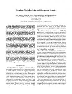
We first evaluate the time required to annotate the database with probabilities. Then, we study the performance of our method for producing clean query answers. Probability Computation We used the technique of Section 4 to produce the probabilities. For the propagation of identifiers, we used the approach that replaces the values of the original keys of the relations with the identifier selected by the tuple matching tool. We experimented with data sets of size 1GB ( ), and values 1, 5 and 25 for the parameter.5 The total execution time for the propagation and probability calculation was, for all databases, less than 30 minutes. This is a reasonable time for an off-line technique. The propagation technique is independent of the number of tuples in each cluster and is only sensitive to the total size of the relations. However, the time to compute probabilities increases as the number of tuples in each cluster increases. This happens since more tuples are used in the computation of the cluster representatives. We experimentally validate this fact with the results in Figure 7. This figure depicts the time taken to propagate and compute the probabilities for the largest relation of our database, the lineItem relation, as well as the time required to perform one linear scan over this relation. The running time for the computation of probabilities grows as the number of tuples increases within each

5 Experimental Evaluation In this section, we evaluate the efficiency of our approach. All the experiments were performed on a machine with 2.8 Ghz Intel Pentium 4 CPU and 1GB of RAM (80% of which was allocated to the database manager). The queries were run on DB2 UDB Version 8.1.8 under Windows XP Professional.

5.1 Data Set Generation In order to assess the efficiency of our techniques on very large data sets, we used a synthetic data generator, the UIS Database Generator.4 This generator was written by Mauricio Hern´andez and has been used for the evaluation of duplicate detection [16]. Given a parameter that controls the number of tuples and a parameter that controls the number of clusters, the generator creates clusters of potential duplicates. We use this generator to produce data that conforms to the schema of the TPC-H specification (http://www.tpc.org/tpch).

5 Notice that the value corresponds to a completely clean database, and hence the computation of probabilities should include the addition of a probability 1.0 to each tuple. However, since this is an off-line procedure, we decided to keep an un-optimized version of our method for , in order to get a baseline reference.

4A copy of the generator can be found at: http://www.cs.utexas.edu/users/ml/riddle/data.html

10

author robert e. schapire author robert e. schapire robert e. schapire author r. schapire schapire, r.e.,

Most frequent values title venue the strength of weak learnability machine learning Top-2 Tuples title venue the strength of weak learnability machine learning the strength of weak learnability machine learning Bottom-2 Tuples title venue on the strength of weak proc of the 30th learnability i.e.e.e. symposium... ’the strength of weak learnability’ machine learning

volume 5(2)

year 1990

pages 197-227

volume 5(2) 5

year 1990 1990

pages 197-227 197-227

volume NULL

year 1989

pages pp. 28-33

52

(1990)

pp. 197-227

Table 4. Example from the Cora data set 900 800

Propagation Probability Calculation

45 40

Execution Time (minutes)

700

Execution Time (sec)

35

600

30 25

500

20

400

15

300

10

200

Linear Scan

5

100 0

0 0.1

1

2

if

25

0.5

1.0

Database Size (GB)

2.0

Figure 11. Execution time over size for Query 9

Figure 7. Offline times for lineItem cluster. When the value of is small, the distance calculation of each tuple to its representative dominates the time, while with larger values, it is the time of the creation of representatives that prevails. Hence, when we move from to , the difference in computation time for the probabilities is mainly due to the merging of more tuples in cluster representatives. This difference is more pronounced as we move from to . Clean Query Answering We performed our experiments on thirteen queries from the TPC-H specification, which contain from one to six joins. In particular, we focused on queries 1, 2, 3, 4, 6, 9, 10, 11, 12, 14, 17, 18, and 20 from the specification. The only change that we made to the queries was removing the aggregate expressions. The queries in the TPC-H specification are parameterized. For all queries, we used the parameters suggested by the standard for query validation. The thirteen queries used in the experiments appear in the Appendix. For each instance, we created indices on the identifier, and ran the DB2 RUNSTATS command on all attributes. In Figure 8, we show the running times of the thirteen queries on a 1 GB database with an average cluster size of 3 tuples. Notice that the overhead of running the rewritten queries is not significant. All queries (except Query 9) execute within 1.5 times the time of the original query. Notably, the rewritten versions of eight queries take less than 1.05 times the execution time of the original query. These are Queries 2, 4, 6, 11, 14, 17, 18, and 20.

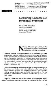
Note that the running times for Query 9 and its rewriting extend well beyond the scale of this graph (the times are indicated in numbers at the top of the figure). This query has six joins and a high selectivity (a large fraction of tuples satisfying its conditions). With a large number of duplicates satisfying the query, the grouping and aggregation of the rewritten query becomes costly. As a result, this rewriting has the highest overhead (1.8 times the time of the original query). In Figure 9, we show the effect of cluster size on the running time. These running times correspond to Query 3, which we show next. This query contains a three-way join, three selection conditions, and an order by clause. select l_orderkey, l_extendedprice*(1-l_discount) as revenue, o_orderdate, o_shippriority from customer,orders,lineitem where c_mktsegment = ’BUILDING’ and c_custkey = o_custkey and l_orderkey = o_orderkey and o_orderdate < ’1995-03-15’ and l_shipdate > ’1995-03-15’ order by revenue desc, o_orderdate

We report results on 1GB instances with 1, 2, 3, 4 and 5. The solid lines correspond to the running times of Query 3 and its rewriting. The running time of both queries increases with the average size of the clusters. The reason for this behavior is that the size of the result set for both 11

4

1.5

4 13.71mins

1

0.5

3.5

3.5

Original Query Rewritten Query Original Query without ORDER BY Rewritten Query without ORDER BY

Execution Time (minutes)

Original Query Rewritten Query

Execution Time (minutes)

Execution Time (minutes)

7.68mins

3

2.5

3 2.5

2

1.5

2 1.5

Query1 Query2 Query3 Query4 Query6 Query10 Query11 Query12 Query14 Query17 Query18 Query20

1

0.5

1 0 0.1

0

0.5 1

Q1 Q2 Q3 Q4 Q6 Q9 Q10Q11 Q12Q14 Q17Q18 Q20

Figure 8.

&

2

3

4

5

Tuples per Cluster

1.0

2.0

Database Size (GB)

Figure 10. Time over DB size

Figure 9. Query 3:

queries increases with the number of tuples per cluster because a tuple may join with more tuples of another relation. Therefore, the order by of the original query and the order by and group by of the rewritten query become more costly. In order to have a better insight into the performance of the rewritten queries, we analyzed the running time of Query 3 and its rewritten version when the order by clause is removed. We show the results in Figure 9 using dashed lines. In this case, the running time of the original query without order by is not affected by the size of the clusters, as expected. On the other hand, the rewritten query is affected by cluster size since it has to perform an additional grouping of the tuples. Finally, we illustrate the scalability of our approach by running the queries on instances of different sizes. In Figure 10, we show the running times of the rewritten queries (with the order by clause) on instances with an average cluster size of 3 and database sizes of 100MB, 500MB, 1GB, and 2GB. Except for Query 3, the running times grow in a linear fashion with the size of the database.

0.5

be the Theorem 1. Let be a rewritable query. Let query obtained by applying the algorithm RewriteClean to . Then, for every dirty database , retrieves the clean answers for on . We first introduce the notion of support set. The support set of a tuple for a query contains all the minimal subsets of the dirty database such that is in the result of applying to . Dfn 8 (support set) Let be a dirty database. Let be a tuple of values, and be a query. We say that is the support set of for on if and there is no subset

of

such that Recall that in the rewritable queries of Definition 7, each relation symbol of the database schema appears in the from clause at most once. Thus, it is easy to see that each element of the support set contains exactly one tuple for each relation symbol that appears in the from clause of the query. be the query obtained by apLet be a query, and plying the procedure of Figure 4 to . In , we obtain the probability of each tuple as follows. For every set of tuples in the support set , we obtain the probability of as the product of the probabilities of all the tuples in . Then, we sum the probabilities of all elements in the support set . Thus, in order to prove the correctness of the algorithm, it suffices to prove that

6 Conclusions We have introduced a novel approach for querying dirty databases in the presence of probabilistic information about potential duplicates. We presented an algorithm that rewrites queries posed over the dirty database into queries that return answers together with their probability of being in the clean database. Our experiments showed that our methods are both intuitive and scalable. This work, however, opens several avenues for further research. First, we would like to extend the class of queries that can be rewritten to consider, for example, queries with grouping and aggregation. We would also like to relax some of the assumptions of our semantics. For example, we would like to extend our techniques to use dependence information across the clusters.

We prove this in Lemma 3. The proof relies on Lemmas 1 and 2 below. In the next lemma, we show how to use the support set in order to compute the sum of the probabilities of all candidate such that . In particular, we show databases that it can be obtained from the probabilities of the candidate databases that contain the elements in the support set .

A Proof of Theorem 1 We now prove Theorem 1, the main technical result of Section 3. 12

Lemma 1 Let be a dirty database, and be a rewritable query. Let be a tuple such that . Let be the support set of for on . Then,

From the above claim, it follows that each candidate database is summed only once in the right-hand side of the formula, and thus we are done. In the next lemma, we show that the probability of an element of the support set corresponds to the sum of the probabilities of all candidate databases that contain . be a dirty database. Let be the set of Lemma 2 Let candidate databases of . Let be a subset of that contains at most one tuple for each relation of . Then,

Proof We must show that the probability of every candidate database that satisfies the query is summed exactly once in the right-hand side of the formula. We are summing the probability of every candidate database that satisfies the query for the following reason. Let be a candidate database of such that . Since , there is a subset of such that and consists of one tuple for each relation symbol of . By definition of support set, . Now, we show that each candidate database is summed only once in the right-hand side of the formula. For this, it suffices to prove the following claim.

and Proof The proof is by induction in the number of clusters of . Base case. Assume that has clusters. Then, is the only candidate database of that contains ; and we are done. Inductive step. Assume that has clusters, for . Let be a cluster of such that none of the tuples of are in . Let be all tuples in . That is, are on the same relation of , and share the same cluster identifier value. Let . Let be the set of candidate databases of . Then, we have that

Claim. Let be a dirty database, and be a rewritable query. Let be a candidate database of such that . Let and be sets from such that and . Then, . The proof is by induction on the number of relations in the from clause of the query. Base case. Assume that has exactly one relation in its from clause. Then, and each contain a single tuple and . Since of the relation , which we denote with the join graph of has only one node, is at the root of the join graph. Let be the cluster identifier of . Since projects on the cluster identifier of the root relation (condition 4 of the definition of rewritable query), we have that . Since is a candidate database, there is exactly one tuple in for each cluster identifier value. Thus, . Inductive step. Let be the join graph of . Since is be a literal whose a rewritable query, is a tree. Let node appears at a leaf of . Let and be tuples of and , respectively. Since is a tree, there is exactly one relation such that there is a join from attributes of to the cluster identifier of . Let be the subgraph of induced by all the nodes of except the one for . Let be a query such that is the query graph of . Let and be the sets from such that and . By inductive hypothesis, . Thus, there is a tuple that appears in both and . Since and join with , and and join on the cluster identifier of (by condition 1 of definition of rewritable query), we have that and share the same cluster identifier values. Since is a candidate database, each cluster identifier value appears in exactly one tuple of . Thus . End of Claim.

and

and Since

has

clusters, by inductive hypothesis,

and Furthermore,

by

definition . Thus,

of

dirty

database,

and We are now ready to prove Lemma 3. Theorem 1, the main result of this section, follows directly from this lemma. Lemma 3 Let be a dirty database, and be a rewritable query. Let be a tuple such that . Let be the support set of for in . Then,

13

Proof By Lemma 1,

select s_acctbal, s_name, n_name, p_partkey, p_mfgr, s_address, s_phone, s_comment from part, supplier, partsupp, nation, region where p_partkey = ps_partkey and s_suppkey = ps_suppkey and p_size = 15 and p_type like ’%BRASS’ and s_nationkey = n_nationkey and n_regionkey = r_regionkey and r_name = ’EUROPE’ order by s_acctbal desc, n_name, s_name, p_partkey

By Lemma 2,

Thus,

Since each tuple in is from a unique relation, we have that all tuples of are chosen independently. Thus, . We conclude that

B Queries used in the experiments

Query 3

The following are the thirteen queries, adapted from the TPC-H specification, that were used in the experiments.

select l_orderkey, l_extendedprice * (1 - l_discount) as revenue, o_orderdate, o_shippriority from customer, orders, lineitem where c_mktsegment = ’BUILDING’ and c_custkey = o_custkey and l_orderkey = o_orderkey and o_orderdate < ’1995-03-15’ and l_shipdate > ’1995-03-15’ order by revenue desc, o_orderdate

Query 1: select l_returnflag, l_linestatus, l_quantity as sum_qty, l_extendedprice as sum_base_price, l_extendedprice * (1 - l_discount) as sum_disc_price, l_extendedprice * (1 - l_discount) * (1 + l_tax) as sum_charge, l_quantity as avg_qty, l_extendedprice as avg_price, l_discount as avg_disc from lineitem where DAYS(’1998-12-01’)-DAYS(l_shipdate) >90 order by l_returnflag, l_linestatus;

Query 4 select o_orderpriority from orders, lineitem where o_orderdate >= ’1993-07-01’

Query 2

14

and days(o_orderdate) < days(’1993-07-01’) + 90 and l_orderkey = o_orderkey and l_commitdate < l_receiptdate order by o_orderpriority

from customer, orders, lineitem, nation where c_custkey = o_custkey and l_orderkey = o_orderkey and o_orderdate >= ’1993-10-01’ and days(o_orderdate) < days(’1993-10-01’) + 90 and l_returnflag = ’R’ and c_nationkey = n_nationkey order by revenue desc

Query 6 select l_extendedprice * l_discount as revenue from lineitem where l_shipdate >= ’1994-01-01’ and days(l_shipdate) < days(’1994-01-01’) + 365 and l_discount >= 0.06 - 0.01 and l_discount = ’1994-01-01’ and DAYS(l_receiptdate) < DAYS(’1994-01-01’) + 365 order by l_shipmode

Query 10 select c_custkey, c_name, l_extendedprice * (1 - l_discount) as revenue, c_acctbal, n_name, c_address, c_phone, c_comment

15

Query 14 select case when p_type like ’PROMO%’ then l_extendedprice*(1-l_discount) else 0 end as promo_revenue from lineitem, part where l_partkey = p_partkey and l_shipdate >= ’1995-09-01’ and DAYS(l_shipdate) 300 and c_custkey = o_custkey and o_orderkey = l_orderkey order by o_totalprice desc, o_orderdate Query 20 select s_name, s_address from supplier, nation, partsupp,

16

part where s_suppkey=ps_suppkey and ps_partkey=p_partkey and p_name like ’forest%’ and s_nationkey = n_nationkey and n_name = ’CANADA’ order by s_name

References [1] R. Ananthakrishna, S. Chaudhuri, and V. Ganti. Eliminating fuzzy duplicates in data warehouses. In VLDB, pages 586– 597, 2002. [2] P. Andritsos, R. J. Miller, and P. Tsaparas. InformationTheoretic Tools for Mining Database Structure from Large Data Sets. In SIGMOD, pages 731–742, 2004. [3] P. Andritsos, P. Tsaparas, R. J. Miller, and K. C. Sevcik. LIMBO: Scalable Clustering of Categorical Data. In EDBT, pages 123–146, 2004. [4] M. Arenas, L. Bertossi, and J. Chomicki. Consistent Query Answers in Inconsistent Databases. In PODS, pages 68–79, 1999. [5] D. Barbara, H. G. Molina, and D. Porter. The management of probabilistic data. IEEE Trans. Knowl. Data Eng., 4:487– 502, 1992. [6] I. Bhattacharya and L. Getoor. Deduplication and group detection using links. In KDD Workshop on Link Analysis and Group Detection, Seattle, WA, Aug. 2004. [7] M. Bilenko and R. J. Mooney. Adaptive duplicate detection using learnable string similarity measures. In KDD, pages 39–48, 2003. [8] A. Cal`ı, D. Lembo, and R. Rosati. On the decidability and complexity of query answering over inconsistent and incomplete databases. In PODS, pages 260–271, 2003. [9] R. Cavallo and M. Pittarelli. The theory of probabilistic databases. In VLDB, pages 71–81, 1987. [10] J. Chomicki and J. Marcinkowski. Minimal-change integrity maintenance using tuple deletions. Information and Computation, 1-2(197):90–121, 2005. [11] T. M. Cover and J. A. Thomas. Elements of Information Theory. Wiley & Sons, 1991. [12] N. Dalvi and D. Suciu. Efficient Query Evaluation on Probabilistic Databases. In VLDB, pages 864–875, 2004. [13] I. P. Fellegi and A. B. Sunter. A theory for record linkage. Journal of the American Statistical Association, 40, 1969. [14] N. Fuhr and T. Rolleke. A probabilistic relational algebra for the integration of information retrieval and database systems. ACM Trans. of Inf. Sys., 15(1):32–66, 1997. [15] H. Galhardas, D. Florescu, D. Shasha, E. Simon, and C.-A. Saita. Declarative data cleaning: Language, model, and algorithms. In VLDB, pages 371–380, 2001. [16] M. A. Hern´andez and S. J. Stolfo. Real-world data is dirty: Data cleansing and the merge/purge problem. Data Mining and Knowledge Discovery, 2(1):9–37, 1998. [17] L. Lakshmanan, N. Leone, R. Ross, and V. Subrahmanian. Probview: A flexible probabilistic database system. TODS, 22(3):419–469, 1997.

[18] A. McCallum, K. Nigam, and L. H. Ungar. Efficient clustering of high-dimensional data sets with application to reference matching. In KDD, pages 169–178, 2000. [19] S. Sarawagi and A. Bhamidipaty. Interactive deduplication using active learning. In KDD, pages 269–278, 2002. [20] W. E. Winkler. The state of record linkage and current research problems. Technical Report RR99/04, US Census Bureau, 1999.

17

Author r. schapire

Title on the strength of weak learnability

r. schapire

on the strength of weak learnability

robert e. schapire r. schapire robert e. schapire robert e. schapire schapire, r. schapire, r. schapire, r. schapire, r. schapire, r. e. schapire, r. e. schapire, r. e. schapire, r. e. schapire, r. e. schapire, r. e. schapire, r. e. schapire, r. e. schapire, r. e. schapire, r.e. schapire, r.e. schapire, r.e. schapire, r.e., schapire, r.e. schapire, robert e. shapire, r. r. e. schapire r. schapire schapire, r. r. e. schapire robert e. schapire robert e. schapire robert e. schapire robert e. schapire r. e. schapire r. schapire robert schapire r. e. schapire r. schapire r. schapire robert e. schapire robert schapire robert e. schapire robert e. schapire r.e. schapire robert e. schapire robert e. schapire robert e. schapire robert e. schapire r. e. schapire r. schapire schapire, r. robert e. schapire robert e. schapire schapire, r.e. shapire, r. e.

the strength of weak learnability the strength of weak learnability combining regression estimates the strength of weak learnability ‘the strength of weak learnability’ the strength of weak learnability the strength of weak learnability the strength of weak learnability ’the strength of weak learnability’ ’the strength of weak learnability’ ’the strength of weak learnability’ the strength of weak learn-ability the strength of weak learnability the strength of weak learnability the strength of weak learnability the strength of weak learnability the strength of weak learnability the strength of weak learnability the strength of weak learn-ability the strength of weak learnability ’the strength of weak learnability’ the strength of weak learnability the strength of weak learn-ability the strength of weak learnability the strength of weak learnability the strength of weak learnability the strength of weak learnability the strength of weak learnability the strength of weak learnability the strength of weak learnability the strength of weak learnability the strength of weak learnability the strength of weak learnability the strength of weak learnability the strength of weak learnability the strength of weak learnability the strength of weak learnability the strength of weak learnability the strength of weak learnability the strength of weak learnability the strength of weak learnability the strength of weak learnability the strength of weak learnability the strength of weak learnability the strength of weak learnability the strength of weak learnability the strength of weak learnability ’the strength of weak learnability’ the strength of weak learnability the strength of weak learnability the strength of weak learnability the strength of weak learnability the strength of weak learnability the strength of weak learnability

Venue proc of the 30th i.e.e.e. symposium on the foundations of cs 42 proc of the 30th i.e.e.e. symposium on the foundations of cs machine learning machine learning 29 machine learning machine learning machine learning machine learning machine learning machine learning machine learning machine learning machine learning mach. learn. machine learning machine learning machine learning machine learning machine learning machine learning machine learning machine learning machine learning machine learning machine learning machine learning machine learning machine learning machine learning machine learning machine learning machine learning machine learning machine learning machine learning machine learning machine learning machine learning machine learning machine learning machine learning machine learning machine learning machine learning machine learning machine learning machine learning machine learning machine learning machine learning machine learning machine learning machine learning machine learning machine learning machine learning

Volume NULL

Year 1989

Pages pp. 28-33

Rank 38

NULL

1989

pp. 28-33

38

5(2) 5 5(2) 5(2) 5(2) 5 5 5 5(2) 5(2) 5(2) NULL 5 5 (2) 5(2) 5(2) 5 5 5 5: 52 5 5(2) 5 5(2) 5 5 5(2) 5 5 5(2) 5(2) 5(2) 5 5(2) 5(2) 5 5(2) 5(2) 5(2) 5(2) 5(2) 5 (2) NULL 5(2) 5(2) NULL vol. 5 num. 2 5(2) 5(2) 5(2) 5(2) 5: vol. 5

1990 1990 1990 1990 (1990) (1990) (1990) (1990.) (1990) (1990) (1990) (1990) (1990) (1990) (1990) (1990) (1990) (1990) 1990 1990 (1990) (1990) 1990 (1990) 1990 1990 NULL 1990 1990 1990 1990 1990 1990 1990 1990 1990 1990 1990 1990 1990 1990 1990 1990 1990 1990 1990 1989 1990 1990 1990 1990 1990 NULL 1990

197-227 197-226 197-227 197-227 197-227 197-227 197-226 197-227 197-227 pp. 197-227 197-227 197-227 197-227 197-227 197-227 197-227 197-227 pp. 197-227 197-227 197-227 pp. 197-227 197-227 197-226 197-227 197-227 197-227 197-227 197-227 197-227 197-227 197-227 197-227 197-227 197-226 197-226 197-227 197-226 197-226 197-227 197-226 197-227 197-227 NULL 197-227 197-227 197-227 pages 28-33 pp. 197-227 pp. 197-227 197-227 197-227 197-226 197-227 pp. 197-227

1 13 31 1 27 9 20 26 17 28 17 36 8 21 5 5 8 24 25 18 37 11 30 19 4 15 22 37 2 2 1 1 4 14 16 23 14 10 1 16 1 1 34 7 1 1 33 35 12 3 1 6 29 32

Table 5. Example from the Cora data set 18