ICUWB 2009 (September 9-11, 2009)
Clock-Offset Tracking Software Algorithms For IR-UWB Energy-Detection Receivers Manuel Flury∗ , Ruben Merz† , Jean-Yves Le Boudec∗ ∗ EPFL, School of Computer and Communication Sciences, † Deutsche Telekom Laboratories, TU Berlin
[email protected],
[email protected],
[email protected]
Abstract— We present a clock-offset tracking algorithm for impulseradio ultra-wide band (IR-UWB) energy-detection receivers. There is a complexity versus performance trade-off for the design of IR-UWB energy-detection receivers: Extremely lowcomplexity energy-detection receivers are built with a large, constant integration duration; they are robust to clock drifts but are sensitive to noise enhancement effects and cannot adapt to channel variations. More sophisticated energy-detection receivers use a shorter integration duration and combine several weighted outputs of the energy collector; they are robust to noise enhancement effects, can adapt to channel variations and offer a much better performance than non-adaptive receivers. However, they become sensitive to clock offsets. Hence, there is a need for lowcomplexity clock-offset tracking solutions to support adaptive energy-detection receivers. Our solution is constructed around the Radon transform, an image processing tool traditionally used to detect line features in images. Our solution is fully compatible with the IEEE 802.15.4a standard, does not increase the hardware complexity of the receiver and reduces the performance loss due to clock offset to less than 0.5 dB.
I. I NTRODUCTION Energy-detection receivers are appealing for impulse-radio ultra-wide band (IR-UWB) use when the focus is on low complexity, low power consumption and inexpensive devices. With a reasonable energy consumption and complexity, energy-detection receivers can exploit the multipath resistance of IR-UWB [1] and its ranging capabilities [2]. Hence, energy-detection receivers fit perfectly the objectives of IEEE 802.15.4a [3], which is an amendment to the IEEE 802.15.4 standard for low data-rate devices with an emphasis on very low complexity and power consumption. The amendment specifies an IR-UWB physical layer that can operate over several bands of 500 MHz (or 1.5 GHz) from 3 to 10 GHz. The implementation of 802.15.4a devices is faced with several challenges. First, the mandatory medium access control layer (MAC) in the standard is based on Aloha and hence, completely uncoordinated; receivers must be robust to occasional interference. Further, with devices mainly operated indoors, receivers should be able to adapt to a time-varying environment and, in particular, a time-varying propagation channel. Finally, with a strong focus on low-priced devices, the underlying hardware can be of average quality. For instance, because of possibly low-quality frequency oscillators used for The work presented in this paper was supported (in part) by the National Competence Center in Research on Mobile Information and Communication Systems (NCCR-MICS), a center supported by the Swiss National Science Foundation under grant number 5005-67322
9781-4244-2931-8/09/$25.00 ©2009 IEEE
clock generation, the standard allows for relative clock offsets as large as 40 parts per million (ppm) [3]. These challenges exhibit the trade-off between robustness to the environment and resilience to clock drifts for the design of energy-detection receivers for IR-UWB physical layers. Extremely low complexity energy-detection receivers are built with a large and constant integration duration, on the order of several tens of nanoseconds [1]; they are robust to clock drifts but are sensitive to noise enhancement effects [4] and cannot adapt to channel variations. More sophisticated energydetection receivers attempt to estimate the power delay profile of the propagation channel. They use a shorter integration duration and combine several weighted outputs of the energy collector according to the estimate of the power delay profile [4], [5], [6]; they are robust to noise enhancement effects, can adapt to channel variations and offer a much better performance than non-adaptive receivers. However, because of the shorter integration duration and consequently higher sampling frequency, they become sensitive to clock offsets. In packet based systems, such as IEEE 802.15.4a networks, there is no global synchronization. For each received packet, the reception of the payload is preceded by a packet detection and timing acquisition phase: Its purpose is (1) to detect the presence of the packet on the wireless medium, (2) to synchronize the clocks of the transmitter and the receiver and (3) to find out when the payload starts. Now, and especially with cheap hardware, the clocks at the transmitter and the receiver drift. For instance with clock drifts of −4 ppm at the transmitter and 18 ppm at the receiver, the overall clock offset is 22 ppm (clock drifts are measured with respect to a global perfect clock.). With a clock frequency of 500 MHz, the clock will be offset by one sample each 90 µs. As we show in Section V, this can severely degrade the performance. For narrow-band physical layers, there are two well-known solutions for addressing clock-offset issues: the phase-locked loop (PLL) and early-late gate synchronizers [7]. However, for energy-detection receivers, they both cannot be used: the PLL cannot be used because of the absence of a carrier and the early-late gate synchronizers cannot be used because they require a correlator. In the specific case of coherent IR-UWB receivers, [8], [9], [10] and [11] address the issue of clock tracking. In [12] clock-offset estimation for coherent and noncoherent IR-UWB receivers are addressed but not tracking. Except for [11], all the previous work require the use of a correlator and are therefore not applicable in our case. Interestingly, [11] relies on the received signal power. However, their
534
solution necessitates the addition of pilot symbols in between modulated data symbols and is tailored for a coherent receiver. Our main contribution in this paper is the development and performance evaluation for IR-UWB energy-detection receivers of (1) a clock-offset compensation solution and (2) a clock-offset tracking algorithm. By tracking, we imply both the estimation and correction of the clock offset. Our tracking algorithm is constructed around the Radon transform [13](Section IV-B), an image processing tool traditionally used to detect line features in images. Our solution does not require any additional pilot symbols, does not increase the hardware complexity of the receiver and naturally takes advantage of the multipath propagation channel for the estimation of the clock offset. Our algorithms are directly applicable to the 802.15.4a standard and the tracking algorithm reduces the performance loss due to clock offset to less than 0.5 dB. The remainder of this paper is organized as follows. We give the system model and assumptions in Section II. We describe our clock offset compensation and tracking algorithms in Section IV, and we evaluate their performance in Section V. We conclude the paper in Section VI. II. S YSTEM M ODEL AND A SSUMPTIONS Without loss of generality, we consider an IEEE 802.15.4a IR-UWB physical layer [3]. We focus on non-coherent, energy-detection reception with binary pulse position modulation (BPPM). An IEEE 802.15.4a packet consists of two parts: a preamble followed by a payload. The preamble is known to the receiver and used for packet detection, timing acquisition, channel estimation and clock-offset tracking. One peculiarity of IEEE 802.15.4a is the different signaling format used in the preamble and the payload. The preamble consists of a sequence of single, amplitude modulated pulses. In contrast, each symbol of the payload is composed of a short, continuous burst of Lb pulses with pseudo-random polarity. The main time unit of a packet is a chip of duration Tc . During the preamble, pulses can only be sent at regular intervals, every L-th chip. The received signal after filtering with a bandpass filter of bandwidth B is then given by X
Npre −1
r(t) =
si · h(t − (1 + ǫ)iLTc − τ ) + w(t)
(1)
i=0
where h(t) is the unknown channel response (including the transmitted waveform, the response of the multipath channel and the bandpass filter), w(t) is a zero-mean AWGN process with power spectral density N0 /2, Npre is the number of pulses in the preamble, si ∈ {−1, 0, +1} is a ternary preamble code used to modulate the preamble pulses, ǫ denotes the relative clock offset between the transmitter and the receiver and τ is the propagation delay. We assume both ǫ and h(t) to be invariant for the duration of one packet. During the payload, the received signal r(t) becomes X
X
Npay −1 Lb −1
r(t) =
i=0
bij · h(t − (1 + ǫ)Ti,j − τ ) + w(t) (2)
j=0
with Ti,j = iTf + ci Lb Tc + ai Tf /2 + jTc and where Npay is the number of symbols in the payload, Tf is the duration
of a symbol, ai ∈ {0, 1} is the i-th symbol of the payload, ci denotes the time-hopping sequence and bij ∈ ±1 is the pseudo-random polarity of the j-th pulse of the i-th symbol specified by the scrambling sequence. On the receiver side, the signal r(t) is squared and integrated. The output of the integrator is sampled at rate 1/T , L Tc and M is a divisor of L. Let γn = nLTc where T = M during the preamble and γn = nTf + cn Lb Tc during the payload, this yields the discrete time signal Z (m+1)T +γn ym,n = [r(t)]2 dt, m = 0, 1 . . . , M − 1. (3) mT +γn
Our receiver employs a traditional synchronization algorithm based on a correlation with the known preamble sequence. After a coarse synchronization, usually achieved on the strongest multipath component, the receiver undergoes a verification phase. If successful, fine synchronization is performed using a back-search algorithm, to obtain a better estimate of the beginning of the signal. The receiver then performs a period of channel estimation where it estimates the energy-delay profile of the channel. At the same time it also begins to look for a special signal sequence called startframe-delimiter (SFD). The SFD is used to designate the end of the preamble and the beginning of the payload. For the demodulation of the n-th data bit an of the payload, the receiver may use the optimum decision rule from [5], [6] M−1 X m=0
ym,n · pm
an =0 ≷ an =1
M−1 X m=0
ym+ Tf
2Tc
,n
· pm
(4)
where the weighting coefficients pm are derived from the energy-delay profile of the channel. A traditional energydetection receiver with an integration window of fixed duration TInt = MLInt Tc can also be used. Then pm = 1 if m ≤ MInt , and 0 otherwise.
(5)
III. W INDOW E XPANSION : C LOCK D RIFT C OMPENSATION A very simple and natural way of addressing clock drift is to gradually expand the length of the integration window of traditional energy-detection receivers at a fixed rate ǫr . The integration window is increased by one sample every 1/ǫr samples. Hence, as the signal drifts, the major part of its energy stays within the window. Assuming we know the precision of the oscillators used in our system, ǫr is typically chosen to be roughly the expected clock drift. A clock-drift estimation is then not required. We call this method Window Expansion. The drawback of this method is noise enhancement due to the increasing integration duration. Window Expansion can be generalized to receivers applying a weighting function such as the one in (4): To expand the window, we smooth the weighting function employed in the decision rule by convolving it with a time-varying window function that increases over time at rate ǫr . Increasing the integration time of traditional energydetection receivers is then equivalent to convolving the rectangular weighting function given by (5) with a rectangular window of increasing length. For the receiver employing the optimum decision rule in (4), we found a triangular window to yield better results than a rectangular one.
535
A
B
20
C 20
0
15
10
10
20
resembling parallel lines at a given angle φ. There is a oneto-one relationship between φ and the clock drift ǫ:
5 10
15
φ = arctan(M ǫ)
20
10
ρ
15
Figure 1D shows our example signal with the two multipath components but this time subject to a clock offset1 of ǫ = 1e − 3. Figure 1E shows the corresponding energy matrix. The signal drifts by one samples every 25 columns (= 1000 samples at M = 40), leading to φ = arctan(1/25) = arctan(40 · 1e − 3).
25 30
5
5
30
0
40
20
0
15
10
10
20
35 0
40 20406080100 120
50 100 150 200
D
pi/2 θ
E
20
F
5 10 15 20
10
B. The Radon Transform: a Tool for Line Detection The (two-dimensional) Radon transform2 is widely used in image processing for line feature detection. We use the common ρ, θ parametrization [16] where the Radon transform R(ρ, θ)[I(x, y)] of the two-dimensional image I(x, y) is Z ∞Z ∞ R(ρ, θ)[I(x, y)] = I(x, y)δ(ρ−x cos θ−y sin θ) dx dy
φ ρ
15
25 30
5
5
30
0
40
←φ→
35 0
40 20406080100 120
50 100 150 200
(6)
pi/2 θ
−∞ −∞
Fig. 1. A relative clock offset ǫ leaves a distinctive pattern resembling parallel lines at an angle φ = arctan(M ǫ) in the energy matrix of an M −periodic signal. In Radon space the maximum is off the right angle by φ.
IV. R ADON T RACKING : A C LOCK O FFSET T RACKING A LGORITHM BASED ON THE R ADON T RANSFORM In this section, we present a clock-offset tracking algorithm, called Radon Tracking, which allows for more sophisticated clock-offset compensation than Window Expansion. A. The Estimation of the Slope of a Line in a Gray-Scale Image is Equivalent to Clock Drift Estimation During the preamble, the samples ym,n can be rearranged in an “energy matrix”, Y = [ym,n ]M×N [14], [15]. The n-th column contains the M consecutive samples corresponding to the n-th pulse of the preamble. This energy matrix is then equivalent to a gray-scale image where ym,n is the intensity of the pixel at coordinate (m, n). Our clock-offset tracking algorithm relies on the following observation: the estimation of the clock drift is equivalent to finding the slope of parallel lines in this gray-scale image. With perfect clock synchronization (ǫ = 0), the signal in (1) is LTc -periodic. Consequently, the discrete signal given by (3) is M -periodic. Accordingly, the energy matrix displays a pattern resembling parallel horizontal lines. These parallel lines correspond to the multi-path components of the signal. Figure 1A shows a discrete signal with 40 samples per frame (M = 40) and two multi-path components. Figure 1B shows the gray-scale image of the corresponding energy matrix. We can observe the two parallel lines corresponding to the two multi-path components. Now, let’s assume for a sample ym,n that the integration window is aligned with the received signal such that it captures the entire energy of a pulse. If the clocks of the transmitter and the receiver exhibit a relative positive (respectively negative) clock drift of ǫ, the alignment of the integration window for the sample ym,n+1 is no longer perfect: Some of the energy “leaks” into the sample ym−1,n+1 (ym+1,n+1 , respectively). In consequence, the energy matrix displays now a pattern
(7) where ρ is the distance from a line to the origin and θ is the angle of the vector from the origin to the closest point on the line. We refer to the (ρ, θ)-parameter space as Radon space. Every point (ρ, θ) in the Radon space corresponds to the ρ θ integral along the line y = − cos sin θ x+ sin θ in the original image I(x, y). Finding lines in a gray-scale image corresponds to finding points with high intensities in Radon space. The basic idea of our algorithm is to apply this principle to our problem of clock-drift estimation. This is illustrated in Figures 1C and 1F that show the Radon transforms of our example signals. Note that the Radon transform can be computed iteratively (see the algorithm in Section IV-D). Hence, we do not need to accumulate the complete energy matrix. In our simulations, we calculate the Radon transform by blocks of M samples. In principle, it can even be calculated sample by sample. C. Pre-Processing to Denoise the Input The Radon transform is already quite robust to noise. However, we further increase this robustness with a pre-processing on the energy matrix before the calculation of the Radon transform. First, we take into account the preamble code by only considering samples ym,n where the corresponding code symbol sn 6= 0. Then, along the rows of Y, we apply a moving ˜ with average filter over the last G pulses, yielding a matrix Y ˜ below a threshold elements y˜m,n . Finally, the elements of Y ¯ with elements ν are set to zero3 . This yields the matrix Y y¯m,n . Because the noise approximatively follows a chi-square distribution, we calculate a threshold ν to reject samples with a probability of more than 5% to consist of noise only: N0 −1 ν= F 2 (1 − 0.05) (8) 2 χ2BT ·G where N0 /2 is the (estimated) noise power spectral density and Fχ22BT ·G (x) is the cumulative distribution function of the chi-square distribution with 2BT · G degrees of freedom. 1 This value is illustrative only; relative clock offsets found in oscillators are usually two orders of magnitude lower. 2 For discrete binary input images it is often referred to as Hough transform. 3 This also speeds up the algorithm as zero valued entries of Y ¯ do not have to be processed in the subsequent steps.
536
D. Computation of the Discrete Radon Transform The Radon transform in (7) is defined for a continuous ¯ = input. Therefore, we transform the discrete matrix Y [¯ ym,n ]M×N into a continuous “image” I(x, y) via nearestneighbor interpolation, i.e. I(x, y) = y¯⌊x⌉,⌊y⌉ where ⌊·⌉ denotes the nearest-integer function. Further, as we cannot store the continuous output of the Radon transform, we discretize the Radon space as follows ρi = i · ∆ρ,
θj = j · ∆θ.
(9)
where ∆ρ is defined with respect to the size of a pixel in the energy matrix i.e., ∆ρ = 1/8 means that we have 8 discrete values per pixel. Hence, we calculate a discrete version R = [Ri,j ] of the Radon transform according to Z ρi+1 Ri,j = R(ρ, θj )[I(x, y)] dρ. (10) ρi
Because the function I(x, y) is piecewise constant, (10) is actually simple to compute. Algorithm 1 shows an outline of the algorithm we use. Furthermore, as the precision of the oscillators is known, the range of interest of both θ and ρ is known. Therefore, the Radon transform can be calculated for only the points of interest, limiting both processing and memory requirements. The Radon matrix that we store has a constant size independent of the length of the observation. The Radon transform is akin to a compression scheme: Instead of the energy matrix, it yields an alternative matrix of a smaller dimension, which still captures all the signal information that is necessary to perform clock-drift estimation. Algorithm 1: Calculates Radon Transform as in (10) ¯ Input: Pixel y¯m,n of Y Output: For each ρ, θ an updated entry Rρ,θ of discrete Radon transform. if y¯m,n 6= 0 then foreach θ do foreach ρ do f ← fraction of pixel with center ym,n lying between lines parametrized by (ρ, θ) and (ρ + ∆ρ, θ); Rρ,θ ← Rρ,θ + f · ym,n ; end end end
intensity averaged over all ρ does not work. Instead, we use the ˆ First, we smooth the matrix following method to determine φ: R by convolving each column with a rectangular window of length W = 2/∆ρ, thus combining the values corresponding to two pixels in the original gray-scale image. Then, we square each entry of the smoothed matrix and compute the column sums. Finally, we set φˆ to the θj corresponding to the column with maximum column sum, i.e. X φˆ = ∆θ · arg max ((rectW ∗ R.,j )[k])2 (11) j
k
where rectW is the rectangular window and R.,j denotes the j-th column of R. F. Continuous Tracking of the Transmitter Clock We are not only interested in the estimation of the clock drift. We also want to continuously compensate for it in order to stay aligned with the packet. Tracking of the transmitter clock is commonly done by adjusting the frequency of the oscillator at the receiver. However, new observations are obtained with an updated sampling frequency after the adjustment of the frequency of the oscillator. This implies a change of the pattern in the energy matrix and a modified Radon transform. A priori, this makes a block by block operation necessary where after each update of the receiver clock: (1) the Radon transform is discarded, (2) a large block of new samples is collected in order to obtain a new Radon transform and (3) the current clock drift is re-estimated on the new Radon matrix. However such a costly approach can be avoided. It is possible to maintain a single Radon matrix by applying a coordinate transform to the Radon space before the update of the receiver clock. This allows for the conservation of the entire signal history and for a continuous estimation and correction of the clock drift. The coordinate transform after k clock frequency adjustments (whose derivation is left out here because of space restrictions) is given by θj (k) =
θj (0) +
k X
∆l
(12)
l=1
ρi (k) = ≈
Pk ρi (0) sin(θj (k)) − l=1 xl sin ∆l sin θj (0) k X ρi (0) − xl sin ∆l
(13)
l=1
E. Angle Estimation by Detection of Maxima in Radon Space As explained in Sections IV-A and IV-B, an estimation of the clock drift is equivalent to finding the estimate φˆ of the angle φ. Thus, we have to look for maxima in the Radon matrix R. Naturally, we should find them around the true angle φ. Due to multipath, there will be more than one such maximum at different values of ρ. We want to take advantage of this property by combining the contributions of several multipath components. However, the column sums of the Radon transform matrix are all equal to a constant value i.e. the integral over the whole image I(x, y). Therefore, the naive approach of choosing φˆ to be the θj with the highest
where ∆l is the angle adjustment corresponding to the l-th clock frequency adjustment, ρi (k) and θj (k) are the transformed coordinates after k adjustments, and xl is the column ¯ corresponding to the l-th point in time index of the matrix Y where the adjustment occurs. The approximation is possible because θj (m) ≈ π/2. In our simulations we start filling the Radon matrix once a coarse estimate of the signal arrival time is available. During the verification phase and fine synchronization, we do not enable tracking but attempt to get a better first estimate of the clock offset. After fine synchronization, we track the transmitter clock until the SFD is found.
537
0
10
−1
10
−1
10
−1
−2
10
PER
10
PER
10
PER
0
0
10
−2
10
−2
10
EDopt, drift
8
EDfix, perfect clock
EDopt + wind. exp., drift
EDvar, perfect clock
EDvar, perfect clock
9
11 SNR [dB]
12
13
14
Fig. 2. PER with perfectly synchronized clocks or with clocks differing by up to ±40ppm. No receiver compensates for drift. EDopt is very sensitive to clock drift but shows optimal performance with perfect clocks. For EDf ix the opposite is true. EDvar is also severely affected by clock drift showing the necessity to compensate clock offsets even in suboptimal receivers. EDf ix and EDvar suffer from noise enhancement.
10
8
9
EDopt+ Radon (∆ρ = 1/2), drift
10
EDopt+ Radon (∆ρ = 1/4), drift EDopt+ Radon (∆ρ = 1/8), drift
EDopt, perfect clock
−4
10
−3
EDvar + wind. exp., drift
10
EDopt, perfect clock
−4
10
−3
EDfix, drift
10
EDvar + wind. exp., drift
EDfix, drift
EDvar, drift −3
EDopt, perfect clock
−4
10
11 SNR [dB]
12
13
14
Fig. 3. EDvar and EDopt show much better robustness to clock drift if simple Window Expansion is used. However, with drift the performance of EDvar is close to EDf ix and 2dB worse than the optimum receiver with perfectly synchronized clocks. Even with Window Expansion, EDopt shows an error floor. More sophisticated mechanisms to cope with drift are necessary.
G. Handling the Residual Clock Drift The signaling format change between the preamble and the payload in IEEE 802.15.4a makes it extremely difficult to maintain a consistent Radon matrix. Hence, we perform clock-drift estimation and tracking only during the preamble of a packet. However, the preamble is long enough such that the residual drift is small. Nevertheless, we find a performance increases if we compensate for this residual drift by employing Window Expansion over the payload (Section III). V. P ERFORMANCE E VALUATION To evaluate the effect of clock drift on energy-detection receivers and the performance of our algorithms, we use a packet-based Matlab simulator. We simulate a full IEEE 802.15.4a system with coarse and fine synchronization, estimation of the energy-delay profile of the channel, SFD detection [3], and data decoding with the (63, 55) ReedSolomon code. For all simulations, the mandatory frequency band 3 low-pulse-repetition-frequency (LPRF) mode is used [3]. The propagation channel is modeled according to the IEEE 802.15.4a residential NLOS channel model [17]. Our main performance metric is the packet error rate (PER) and we simulate the maximum allowable packet length of 1016 bits per packet. We use the default length of the preamble of 72 code repetitions (including 8 for the SFD). The signalE to-noise ratio (SNR) is defined as SNR = Np0 where Ep is the received energy per pulse (after the convolution of the pulse with the impulse response of the channel). The physical layer is simulated with an accuracy of 100 ps (a simulation sampling frequency of 10 GHz). We assume oscillators with a drift ǫ uniformly distributed in the range of ±20 ppm, resulting in relative clock offsets between transmitters and receivers of up to ±40 ppm. For the receiver, we mainly focus on the optimal receiver (EDopt ) detailed in [6] with T = Tc = 2 ns resulting in a 500 MHz sampling frequency. For comparison purposes, we also simulate two reference receivers: one with a fixed integration time Tint = 128ns (EDf ix ), and one with an integration time that was optimized for our scenario
10
8
9
10
11 SNR [dB]
12
13
14
Fig. 4. PER if Radon Tracking is used. Curves are for EDopt with different values of the discretization step ∆ρ. We also show the two curves from Figure 3 giving best performance with and without drifting clocks. Our algorithm performs well, with ∆ρ equal to 1/8 and 1/4. We only loose about 0.5dB with respect to the optimal curve.
(EDvar ). Without drift, this optimized integration time was found to be 56 ns, which is roughly the channel spread of the residential NLOS model. Further, EDvar may use Window Expansion to increase the integration time at a constant rate ǫr (but not EDf ix ). Note, that for both EDvar and EDf ix , we do not simulate the preamble. Instead, we assume that a perfect synchronization puts the integration window such that it captures a maximal amount of energy. Figure 2 shows the performance degradation due to a relative clock offset up to ±40 ppm when no clock-offset compensation is used. We can clearly see the trade-off between noise enhancement and robustness to clock drift. With perfect clocks, EDopt outperforms the other receivers, even though the curves for EDf ix and EDvar were obtained with a perfect synchronization. On the other hand, EDopt is very sensitive to clock drifts: Indeed they cause misalignments of the weights pm (see (4)) that strongly degrade the performance. Interestingly, EDvar is also severely affected by clock drift, although to a lesser extent than EDopt . EDf ix , on the other hand, is barely affected due to its long integration time. Figure 3 shows the improvement achievable through Window Expansion. We found ǫr = 32 ppm to give best performance for EDvar and ǫr = 40 ppm for EDopt . With drifting clocks, EDvar with Window Expansion performs hardly better than EDf ix , which amounts to a loss of about 2 dB with respect to the optimum curve for perfectly synchronized clocks. EDopt with Window Expansion, on the other hand, still shows an error floor. Although Window Expansion gives some improvement, it is definitely not sufficient. Figure 4 shows the performance of Radon Tracking. We show results for different values of the discretization step ∆ρ. The angular resolution ∆θ is fixed to the angle corresponding to a 1 ppm drift. To increase robustness against noise we combine G = 32 preamble pulses and to account for residual drift we set ǫr = 2 ppm. We also show reference curves for EDopt with perfect clocks, and EDvar with Window Expansion and drifting clocks. The results show that our algorithm performs extremely well with a loss of only 0.5 dB with ∆ρ = 1/8 with respect to the optimal curve for perfect
538
3
synchronized clocks. Interestingly, the same is true for a receiver that only employs Window Expansion. We attribute this mostly to the fact that we continuously update the estimate of the channel energy-delay profile during the preamble. Large misalignments of the weights pm are therefore not possible during the preamble and the small ones are recovered through Window Expansion. In contrast to data decoding, clock-offset tracking is thus not strictly required for synchronization alone. Even in ranging applications, however, this is only of limited interest because one might need to determine the clock offset in order to account for it in the range calculations.
0.2
Percentage of Packets
Median of Residual Drift (ppm)
2.5 2 1.5 1 ∆ρ = 0.5 ∆ρ = 0.25 ∆ρ = 0.125
0.5 0
0.1
7
8
9
10
11
12
0
SNR [dB]
0
1
2
3
4
5
6
7
Fig. 5. Left: Median and 95% confidence intervals of the (absolute) residual drift of Radon Tracking at the end of the preamble. Finer discretization leads to a better clock drift estimate. With ∆ρ = 1/8 we do almost as good as we theoretically can at 12 dB considering that we only use a resolution of 1ppm. Right: Distribution of absolute residual drifts of packets after the preamble with Radon Tracking. Distribution shown is for ∆ρ = 1/8 and SNR = 12 dB. 0
10
−1
10
SER
VI. C ONCLUSION
Absolute Value of Residual Drift (ppm)
−3
EDopt, drift EDopt+ Radon (∆ρ = 1/8), drift EDopt + wind. exp., drift
−4
10
5
F UTURE W ORK
R EFERENCES
−2
10
10
AND
We have shown that to prevent a considerable performance loss, clock drifts need to be addressed for energy-detection receivers. We analyzed two solutions: Window Expansion and Radon Tracking. The latter is a clock-offset tracking algorithm based on the Radon transform that yields excellent performance. For future work, we believe that this algorithm is even more versatile and could be used for channel estimation and synchronization purposes. We also want to analyze and improve its performance with multi-user interference.
EDopt, perfect clock 6
7
8 SNR [dB]
9
10
11
Fig. 6. Synchronization error rate accounting for false alarms and missed detections for EDopt . With clock-offset tracking enabled, the error floor disappears and performance is within 0.3 dB of the one with perfect clocks. With only Window Expansion we interestingly have similar performance.
clocks. For ∆ρ = 1/4 the performance is still similar. If we further increase ∆ρ we get an additional loss of 0.5 dB at ∆ρ = 1/2. A finer discretization yields a better estimate of the clock drift. This is confirmed by Figure 5 (Left), where we show the median of the absolute value of the residual drift at the end of the preamble. At 12 dB the median is as low as 0.65 ppm which is not far from the optimal value considering that our algorithm has a resolution of 1 ppm. Figure 5 (Right) shows the corresponding distribution of the absolute values of the residual clock drift for ∆ρ = 1/8 at 12 dB. Only a few packets have a residual drift of more than 2 ppm. This justifies our choice for ǫr = 2 ppm. For both ranging and communication, synchronization is the most crucial part for the reception of a packet. Figure 6 shows the effect of clock drift on the synchronization error rate (SER, false alarm and missed detection) for EDopt . If the receiver does not use tracking, we can see an error floor at about 30% packets lost due to synchronization errors, mainly because the estimated channel energy-delay profile used in SFD detection is now misaligned due to drift. With Radon Tracking (here shown for ∆ρ = 1/8, results for other values of ∆ρ were practically identical), the error floor disappears and the performance is only 0.3 dB worse than with perfectly
[1] S. Dubouloz, A. Rabbachin, S. de Rivaz, B. Denis, and L. Ouvry, “Performance analysis of low complexity solutions for UWB low data rate impulse radio,” in IEEE ISCAS, May 2006. [2] C. Duan, P. Orlik, Z. Sahinoglu, and A. F. Molisch, “A non-coherent 802.15.4a UWB impulse radio,” in IEEE ICUWB, September 2007. [3] IEEE Computer Society, LAN/MAC Standard Committee, “IEEE P802.15.4a/D7 (amendment of IEEE std 802.15.4), part 15.4: Wireless medium access control (MAC) and physical layer (PHY) specifications for low-rate wireless personal area networks,” Jan. 2007. [4] M. Weisenhorn and W. Hirt, “ML receiver for pulsed UWB signals and partial channel state information,” in IEEE ICU, 2005, pp. 6 pp.+. [5] A. A. D’Amico, U. Mengali, and E. Arias-De-Reyna, “Energy-detection UWB receivers with multiple energy measurements,” IEEE Trans. Wireless Commun., vol. 6, no. 7, pp. 2652–2659, 2007. [6] M. Flury, R. Merz, and J.-Y. Le Boudec, “An Energy Detection Receiver Robust to Multi-User Interference for IEEE 802.15.4a Networks,” in IEEE ICUWB, 2008. [7] J. G. Proakis, Digital Communications, 4th ed. McGraw–Hill, 2001. [8] C.-C. Chui and R. A. Scholtz, “Optimizing tracking loops for uwb monocycles,” in IEEE Globecom 03, vol. 1, 2003, pp. 425–430 Vol.1. [9] S. Farahmand, X. Luo, and G. B. Giannakis, “Demodulation and tracking with dirty templates for UWB impulse radio: algorithms and performance,” IEEE Trans. Veh. Technol., vol. 54, no. 5, 2005. [10] B. Zhen, H.-B. Li, and R. Kohno, “Clock offset compensation in ultrawideband ranging,” IEICE Trans. Fundam. Electron. Commun. Comput. Sci., no. 11, pp. 3082–3088, 2006. [11] L. Huang, El, O. Rousseaux, and B. Gyselinckx, “Timing tracking algorithms for impulse radio (IR) based ultra wideband (UWB) systems,” in WiCom, 2007, pp. 570–573. [12] A. Wellig and Y. Qiu, “Trellis-based maximum-likelihood crystal drift estimator for ranging applications in uwb-ldr,” in IEEE ICUWB, 2006. ¨ [13] J. Radon, “Uber die Bestimmung von Funktionen durch ihre Integralwerte l¨angs gewisser Mannigfaltigkeiten,” Ber. S¨achs. Akad. der Wissenschaften, Leipzig, Math.-Phys. Klasse, vol. 69, pp. 262–267, 1917. [14] Z. Sahinoglu and I. Guvenc, “Multiuser interference mitigation in noncoherent uwb ranging via nonlinear filtering,” EURASIP Journal on Wireless Communications and Networking, pp. 1–10, 2006. [15] D. Dardari, A. Giorgetti, and M. Z. Win, “Time-of-arrival estimation of uwb signals in the presence of narrowband and wideband interference,” in IEEE ICUWB, 2007, pp. 71–76. [16] R. O. Duda and P. E. Hart, “Use of the Hough transformation to detect lines and curves in pictures,” Commun. ACM, vol. 15, no. 1, 1972. [17] “IEEE 802.15.4a channel model - final report, document 04/662r0,” http: //www.ieee802.org/15/pub/TG4a.html, November 2004.
539