Closed-loop Field Development Optimization - Stanford University

Closed-loop Field Development Optimization Mehrdad Gharib Shirangi Department of Energy Resources Engineering Stanford University

Abstract In this paper, a framework for sequential well placement optimization under time-dependent uncertainty is introduced. Most of the previous studies on well placement optimization considered a fixed reservoir model, or in some cases, a fixed set of reservoir models. Due to the fact that new wells are usually drilled sequentially in time rather than simultaneously, after starting production/injection for each new well, one can update the reservoir models by history matching the data from all the existing wells, including the new well. Future well locations are determined by performing a reoptimization over the updated realizations for the remaining reservoir life. This procedure is called as “closed-loop field development” because of its similarity to “closedloop reservoir management”. The closed-loop field development cycle is repeated until drilling additional wells does not increase the expected life-cycle NPV. An example is presented that demonstrates the application of closed-loop field development.

Introduction Closed-loop reservoir management (CLRM) (Brouwer and Jansen, 2004; Sarma et al., 2006; Jansen et al., 2009; Wang et al., 2009; Peters et al., 2010) has two major steps: data assimilation and production optimization. In the data assimilation or history matching step, the objective is to reduce uncertainty in reservoir description by assimilating the production data and/or seismic data. The uncertainty in the reservoir description is modeled by generating a set of plausible realizations of the reservoir model. In the production optimization step, an optimal well control strategy is found that maximizes the expectation of net present value (NPV) or the expectation of oil recovery over a set of reservoir models (van Essen et al., 2006). Fig. 1 shows the CLRM cycle. The CLRM cycle is repeated over the life of the reservoir. CLRM is mainly for the secondary stage of hydrocarbon production where water flooding or gas injection is performed. CLRM can also be used for tertiary recovery where enhanced oil recovery (EOR) techniques are used for hydrocarbon production. A good choice for the number of wells, well type, well location, drilling sequence, and well settings (well controls) can significantly increase the hydrocarbon recovery or the NPV. Besides the optimization of continuous well settings which is considered in CLRM, the remaining decision variables are determined in “field development optimization”. Most of the methods in the literature considered optimizing only a few of the decision parameters mentioned earlier. For well 1

2

Set Controls & Operate Collect Reservoir Data

Optimize Well Settings

Update Models

Figure 1: Schematic layout of closed-loop reservoir management (CLRM). placement optimization, both gradient-based methods (Wang et al., 2007; Zhang et al., 2010; Handels et al., 2007; Sarma and Chen, 2008) and derivative-free methods (Burak et al., 2002; Ozdogan and Horn, 2006; Onwunalu and Durlofsky, 2009; Bellout et al., 2012) were considered. Isebor and Durlofsky (2012) introduced a hybrid PSO-MADS optimization method for the joint optimization of well location and controls. Their method has both the advantages of PSO (particle swarm optimization) as a global optimization algorithm, and the rather fast convergence of mesh adaptive direct search (MADS) algorithm. Recently, Isebor and Durlofsky (2013) provided a formulation to determine the optimal type of the wells and the optimal drilling sequence in addition to the optimal number, location and timevarying controls of the wells. Their algorithm is the most general field development optimization algorithm introduced so far. They introduced a ternary categorical variable that can take values of {−1, 0, 1} corresponding to drilling an injection well (−1), not drilling (0), and drilling a production well (1). Their method is used in the computational results presented in this work. As the subsurface geology is highly uncertain, the reservoir model is usually described by a set of realizations. In order to consider the uncertainty in reservoir description, the objective function is defined as the expectation of NPV over a set of realizations. When a large number of geological realizations are required to capture the uncertainty, retrospective optimization approach can be used to significantly reduce the number of simulation runs (Wang et al., 2012). Wang et al. (2012) applied the retrospective optimization (RO) approach to the well placement optimization problem, using PSO. RO is based on solving a sequence of optimization subproblems with increasing number of realizations instead of solving one optimization problem with all realizations

3 included. They applied k-means clustering for choosing a set of representative realizations at each subproblem. Shirangi and Mukerji (2012) and Shirangi (2012) investigated the application of the RO approach of Wang et al. (2012) for the production optimization problem within the CLRM context. Their results show that the well control optimization problem can be performed on a set of few representative realizations and a RO approach does not necessarily improve the results significantly. Ozdogan (2004) and Ozdogan and Horn (2006) coupled the well placement optimization with the history matching step, and proposed the “multiplacement with pseudo-history” method. For optimization, they used a hybrid algorithm combined of GA (generic algorithm), polytope algorithm and kriging proxy. The well placement formulation of Ozdogan and Horn (2006) does not include the optimal drilling sequence, and only one optimization takes place in their method. For history matching, they used the gradual deformation method (Roggero and Hu, 1998). In this paper, the idea of closed-loop reservoir management is extended to well placement optimization. A framework called “closed-loop field development” (CLFD) is introduced that incorporates a model updating step into sequential well placement optimization. In the next section, CLFD and its components are described. Next, computational results are presented with a synthetic example that demonstrates the application of CLFD. The last section is allotted to conclusions and future work.

Closed-loop Field Development In this section, the general idea of closed-loop field development is illustrated first, and then notations are introduced to further explain the details of the methodology.

General Idea As stated earlier, field development is performed over time, and wells are usually drilled sequentially rather than simultaneously. However, most of the literature is on developing new methods for optimization of placement of several wells, ignoring the variables of drilling sequence and the effect of time-dependent uncertainty of geological models. As field development optimization is performed over time, and reservoir models can be updated with data from the new wells, field development optimization and model updating can be combined into one framework called closed-loop field development (CLFD). Fig. 2 shows the CLFD cycle which is similar to the CLRM cycle shown in Fig. 1. Both CLRM and CLFD involve history matching and optimization, however the components of CLFD is more complicated due to the following reasons: 1. In CLRM, well locations are fixed, and data assimilation is rather easy to perform. In CLFD, when a new well is drilled, one should be able to update the current realizations of the reservoir model with the hard data (observed facies or measured values of porosity/permeability) from the new well. In addition, the realizations should also be conditioned to the time-dependent production data from all the existing wells including the new well. 2. The optimization step of CLFD contains categorical, discrete and continuous variables which makes it significantly more complicated than optimizing the continuous well settings

4

Drill New Well

Collect Reservoir Data

Optimize Well Placement

Update Models

Figure 2: Schematic layout of closed-loop field development. in CLRM.

Proposed Methodology Here, we explain the basic methodology of CLFD. Let t1 , t2 , . . . ti , . . . tn denote a discrete series, where ti denotes the time (in Days) that the production/injection for the ith well is started. For now, we consider that the location and type (injector/producer/null) of the ith well is decided at time ti−1 . The type of the well would be “null” when the optimization package determines no well should be drilled at time ti . CLFD involves the following components: 1. Optimization of well locations and controls: the optimization package should determine the optimal drilling sequence in addition to optimal locations and controls and optimal well types. Although, at each ti the optimization determines the locations and controls of all the wells to be drilled and the future controls of all the existing wells, only the next one well is drilled according to the provided solution, i.e., only the location of the (i + 1)th well is determined at time ti . This is because at time ti+1 , the realizations will be updated with the production history of all the existing wells in the time period (ti , ti+1 ) and a reoptimization is performed over the updated models. Again, the result of the last reoptimization determines the location of the next one well, and the CLFD cycle is repeated. Note that the solution of the optimization at time ti is used as the initial guess for the optimization problem at time ti+1 .

5 The optimization method should be computationally efficient as the optimization is repeated several times. 2. History matching data: each newly drilled well at time ti provides some static data, e.g., hard data (or observed facies). It also provides some time-dependent production data observed from this point on. At time ti+1 , realizations should be updated with all the new data in the period (ti , ti+1 ) including the data from the ith well. Hard data is usually used as conditioning data when generating simulations of rock property fields with geostatistics. However, as the realizations are already history matched for all the data up to time ti , it would be computationally more efficient to update the current realizations with the new data rather than generating new realizations using geostatistics and then history matching them with all the production history from time 0 to ti+1 . In other words, when history matching realizations at time ti+1 , the current realizations (conditioned to all the data up to time ti ) are used as initial guesses. As the total history matching period is (0, ti+1 ), the prior realizations are the same as the realizations at time 0. In this formulation, hard data would have to be included in the history matching objective function similar to the formulation of Chu et al. (1995). This is due to the fact that hard data which is usually the measured values of porosity and permeability (or observed facies) at well gridblocks, is associated with some measurement errors and hence an exact match should not be forced. 3. Another important component of CLFD is the integration of seismic data. Seismic surveys are performed a few times during the reservoir life for reservoir monitoring. Simulating seismic surveys involves using a rock physics model. As a remark, note that after history matching realizations with all the data up to time ti , all the simulation state variables, i.e., phase pressures and saturations, are saved into restart files. During optimization, all reservoir simulations start at time ti until the end of reservoir life. This would enhance the computational efficiency by avoiding unnecessary simulation of the reservoir for the time period before ti . CLFD provides a framework that different methods of history matching production and seismic data and different methods of field development optimization can be used and compared. CLFD is a sequential decision making process. At each time ti , one should decide on some decision parameters in the time period (ti , ti+1 ). Decision parameters include the location of the next well to drill, and the controls of all the existing wells.

History Matching Production Data History matching for generating a realization of reservoir model is usually performed by minimizing an objective function that quantifies the mismatch between the observed data and production history. For two-point (TP) geostatistical models, history matching is usually performed by using gradient-based optimization algorithms (Sarma et al., 2006; Gao et al., 2006) or derivative-free methods (Fern´andez Mart´ınez et al., 2012; Fern´andez-Mart´ınez et al., 2011). The posterior pdf of model parameters conditioned to observed data can be written as f (m|dobs ) = a exp(−O(m)),

(1)

6 where a is the normalizing constant and O(m) which is referred to as the total objective function, is give by 1 1 −1 −1 (m − mprior ) + (g(m) − dobs )T CD (g(m) − dobs ) O(m) = (m − mprior )T CM 2 2 = Om (m) + Od (m), (2) where the first term is the model mismatch term and the second term is the data mismatch term; mprior is the mean of the prior model, CM denotes the prior covariance matrix, g(m) is the predicted data vector; dobs denotes the Nd -dimensional vector of observed data, CD denotes the Nd ×Nd covariance matrix for the measurement error. The maximum a posteriori estimate (MAP) is the model that maximizes Eq. 1 or equivalently minimizes Eq. 2. The MAP estimate represents the mode of the a posteriori pdf. For models based on TP geostatistics, randomized maximum likelihood (RML) (Oliver et al., 1996) is used for sampling the a posteriori pdf. Generating Ne posterior realizations using RML, involves minimizing Ne objective functions, where the objective function for each realization has the following form: Oj (m) = Om,j (m) + Od,j (m) 1 1 −1 −1 (m − muc,j ) + (g(m) − duc,j )T CD (g(m) − duc,j ), (3) = (m − muc,j )T CM 2 2 where muc,j ∼ (mprior , CM ) is a realization from the prior pdf, duc,j is the vector of perturbed observed data, which is a sample from N (dobs , CD ). Based on the results discussed in Oliver et al. (2008), if mc is the conditional model obtained at convergence of an optimization algorithm, we expect ON (mc ), the normalized objective function evaluated at mc , satisfy p p (4) 1 − 5 2/Nd ≤ ON (mc ) ≤ 1 + 5 2/Nd , where the normalized objective function is defined for the jth realization by ON,j (m) =

Oj (m) . Nd

(5)

Note that realizations with high values of normalized objective function (ON (m)) have poor data matches. A high value of ON (m), is due to a high value of Od,j (m) in Eq. 3, and a high value of Od,j (m) means that this model is not likely. In addition, a model with a high value of ON (m) gives a small value of the posterior pdf which suggests that this model is a sample from a low probability region (Emerick, 2012). In this work, a quasi-Newton method with a damping procedure is used for minimizing each objective function in the form of Eq. 3 (Gao and Reynolds, 2006). Here, the damping procedure is briefly described. It is known that large changes in model parameters in history matching problems add roughness to the model that is hard to remove at late iterations and hence it will result in convergence to a model that is far from the true model. In order to prevent large changes in model parameters at early iterations of optimization, a damped objective function is minimized, i.e. Eq. 3 is modified to Oj (m) = Om,j (m) + αOd,j (m), (6)

7 where α is the damping factor calculated from  5 , ON,j (m) > 5 ON,j (m) . α= 1, ON,j (m) < 5

(7)

The damping procedure is performed in the following way. Calculate α from Eq. 7 and minimize the damped objective function with this fixed α. After 5 or 10 iterations of the optimization algorithm, recalculate the damping factor α, and minimize the new objective function for another 5 to 10 iterations. This is repeated until the normalized objective function is less than 5 where the actual objective function with no damping is minimized.

Robust Field Development Optimization CLFD involves optimization over a set of reservoir models, the so called “robust optimization”. For a fixed reservoir model, the NPV for the field development optimization problem, denoted by J(u, mk ), is defined by J(u, mk ) =

NP L X X n=1

j=1

n (ro qo,j

−

n cwp qw,j )

−

NI X

n cwi qwI,i

i=1

−



∆tn (1 + b)tn /365

NP X j=1

N

I X CP CI , (8) − t /365 j (1 + b)ti /365 (1 + b) i=1

where the first part is the same as the production optimization NPV, and the second part is to account for the drilling cost. In Eq. 8 mk is a vector of model parameters for the k-th realization of the reservoir model; L is total number of simulation time steps; u is the vector of decision parameters; NP and NI denote the number of producers and injectors, respectively; the scalers ro , cwp and cwi all have the unit $/STB and denote respectively, the oil revenue, the cost of n denotes the average injected water handling produced water and the cost of water injection. qwI,i n n , respectively denote the average of the ith injector at the nth simulation time step; qo,j and qw,j produced oil and produced water of the jth producer at the nth simulation time step, all in STB/D. b is the annual discount rate. CI is the cost of drilling an injector, while CP is the cost of drilling a producer; ti and tj respectively denote the drilling time of the ith injector and the jth producer in Days. In robust optimization, the expectation of NPV over a set of reservoir models is optimized. Let Mi denote the Nm × Ne matrix of realizations of reservoir model updated at time ti of CLFD, i.e., Mi = [m1,i , m2,i . . . mNe ,i ], (9) where mj,i is the Nm -dimensional column vector of the jth reservoir model updated at time ti , and Ne denotes the number of realizations of the reservoir model. The robust optimization problem can be written as follows. ¯ Mi ), maximize J(u, Ne X ¯ Mi ) = E[J(u, m)] = 1 J(u, J(u, mj,i ), Ne j=1

(10)

8

6 10 4 20 2 30 40

0

10

20

30

40

−2

Figure 3: True log-permeability field. subject to the constraints: ek (u, mj,i ) = 0, k = 1, · · · , ne ,

(11)

ck (u, mj,i ) ≤ 0, k = 1, · · · , ni ,

(12)

up ulow k ≤ uk ≤ uk , k = 1, · · · , nb ,

(13)

where ne denotes the number of equality constraints, ni denotes the number of inequality constraints, and nb denotes the number of bound constraints. Let ui denote the optimal decision ¯ i , Mi ) denotes the optimal parameters after performing optimization at time ti . Therefore, J(u value of the objective function at time ti . As mentioned earlier, the initial guess for optimization at time ti , is the optimal solution from the previous time step. With the notations introduced here, the initial guess at time ti is ui−1 .

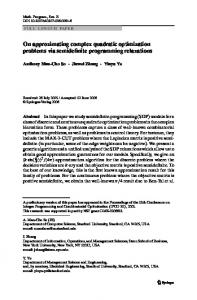
Computational Results This example pertains to a two-dimensional horizontal reservoir model with 40 × 40 uniform grid. True log-permeability field is shown in Fig. 3, while porosity is uniform and equal to 0.3 at all gridblocks. In this example, the idea of closed-loop field development is illustrated. Geostatistical parameters of this example are assumed to be known. The ln(k) field has a spherical variogram, with a maximum range of 23 gridblocks in the NorthWest direction and a minimum range of 7 gridblocks in the NorthEast direction. The gridblock dimensions are 4x = 4y = 150 ft, 4z = 15 ft. Table 1 shows the optimization parameters for this example. In this table Cwell denotes the cost of drilling a well. Other parameter were defined earlier. Fluid properties and variogram parameters are assumed to be known, hence the permeability field is the uncertain parameter of the reservoir model in this example. The initial reservoir pressure is 4870 psi. Initially the reservoir is at irreducible water saturation Swc = 0.15. The objective is to develop the field with maximum 8 wells at their optimal locations with optimal drilling sequence and operate the wells with optimal settings. As only one drilling rig is available to operate on the field, one well can be drilled at a time, and it takes 210 days to drill a

9 Table 1: Optimization parameters of Example 1. parameter Cwell b ro cwp cwi

value $ 10 MM 0.1 $/STB 90 $/STB 10 $/STB 8

new well, hence the discrete times that the ith well (i = 1, 2 . . . 8) is started to produce or inject are {t1 , t2 , t3 . . . t8 } = {0, 210, 420, . . . 1470}. (14) The optimization consists of 8 consecutive time steps, each of which is 210 days long, followed by a final time step of 1320 days. Hence the total reservoir life is 3000 days. The available static information is 3 hard data in form of the value of the permeability at 3 different locations as shown in Fig. 11 with H-1, H-2 and H-3 in the subfigure corresponding to “0 days”. Initial realizations conditioned to the hard data are generated using sequential Gaussian simulation (SGSIM). The available dynamic data here is production history observed at 15 day intervals. Observed data would include the injection rates of the existing injectors and water rates and oil rates of existing producers. Synthetic observed data are generated by adding Gaussian random noise to the true data, where the true data are the simulator output when it is run with the true model. The standard deviation of noise (measurement error) is 2% of rates, i.e., σqw = 0.02qw . The minimum measurement error for the rates is specified to 0.5 STB/D while the maximum measurement error is 3 STB/D. As the optimization software that is used here (Isebor and Durlofsky, 2013) takes many hours to find an optimal solution, the optimization is performed over 5 realizations only, i.e., the expectation of NPV over 5 realizations is optimized. These realizations were chosen randomly and no clustering was performed to choose a set of representative realizations. Nonlinear constraints such as maximum water injection rate or maximum liquid production rate are not specified. The injection and production BHP is subject to bound constraints, as shown in Table 2. Table 2: Bound constraints on BHP of wells. parameter value Injection BHP range 6000 − 9000 Production BHP range 1500 − 4500

Fig. 4 shows the general strategy for field development optimization of this example. Note that in Fig. 4 before performing the reoptimization, reservoir models are updated with all the production history available since time zero. The first optimization is performed prior to the start of production to determine the initial solution to the field development optimization. The production starts at time 0 with producer P-1. At this time (0 days) drilling of the second well

10

Optimize for wells 1‐8  Optimize for  Drill well 1, (Well 1 starts  producing/injecting)

start  start drilling well 2

0‐210 days         (Production Data  from well 1)

(Well 3  (Well 3 starts producing/injecting) producing/injecting)

History match data, reoptimize for wells 4‐8,  Start drilling well 4

210‐420 days       (Production Data  from wells 1,2)

420‐630 days        (Production Data  from wells 1,2,3)

(Well  starts producing/injecting) (Well 2 starts producing/injecting)

History match data,  reoptimize for wells 3‐8,  Start drilling well 3

Figure 4: General strategy for field development optimization of Example 1. at the location from the solution to the first optimization is also started. Hence, the location of the first two wells are determined from the initial optimization on prior realizations.

Change of Optimal Solution During Update Steps of CLFD As discussed earlier, after updating the realizations at each step, the optimization is performed on the updated models starting with an initial guess. We first performed the field development optimization on the true model (mtrue ). The optimal solution when optimizing on the true model is denotes by u∗ . The optimal NPV when optimizing on the true model, J(u∗ , mtrue ), is shown by solid black line in Fig. 5. This figure also shows ¯ i , Mi ), and the value of expected NPV for the initial guess the optimal expected NPV, J(u ¯ J(ui−1 , Mi ) at each ti = 0, 210 . . . 1260 days. As discussed earlier, the initial guess at each time step ti corresponds to the optimal solution from the previous step (ui−1 ). The initial guess at time zero is chosen by user. Preferably, the initial guess for well locations at time zero should be a standard pattern. Mi is a matrix that contains the realizations of the reservoir model updates at time ti . The optimization solution (ui ) in this example determines the optimal number, type, location, controls and the optimal drilling sequence of the wells. At each optimization step, optimization parameters corresponding to the location of the wells already drilled or the well controls of the past time, are specified as constant parameters. Fig. 6 shows the optimal expected NPV and the corresponding “NPV for the true model” versus the update steps of CLFD. As the true model is known in this synthetic example, we

11 7

x 10 16 14 NPV ($)

12 10 8 J(ui−1 , Mi )

6

J(ui , Mi )

4 2

J(u* , mtrue ) 0

210

420

630 840 Time (Days)

1050

1260

¯ i , Mi ), and “NPV for the corresponding initial guess”, Figure 5: The optimal NPV, J(u ¯ i−1 , Mi ), versus the update steps of CLFD. J(u take the optimal solution (ui ) and run the simulator with the true model (mtrue ) and ui . Hence J(ui , mtrue ) corresponds to the NPV that would be obtained in reality if the optimal development plan was to be implemented. In Fig. 6, the difference between the NPV for the true model, J(ui , mtrue ), and the optimal ¯ i , Mi ), is significant at 0 days (i = 1). As stated earlier, the initial realizations are NPV, J(u only conditioned to 3 hard data. A significant increase of 62% in the NPV for the true model is obtained at 210 days, where the realizations are conditioned to the production data from producer P-1. At t = 420 days, the NPV for the true model has a small decrease. Note that there is no guarantee that the NPV for the true model J(ui , mtrue ) be greater than J(ui−1 , mtrue ). This is because the optimization at each ti is performed on a different set of models (Mi ), the NPVmodel relationship is very complex, the field development objective function is highly nonlinear, and the optimization package that is used here has a stochastic nature. In Fig. 6, no NPV is shown at 630 days. The optimal solution form optimization at time 420 days determined that the next well type is “null”, i.e., no well should be drilled at the next time step which is 630 days. The NPV for the true model at time t7 = 1260 days is the highest which shows about 70% improvement over the one at 0 days. Note that the realizations at t7 are conditioned to all the production data from the first 5 wells and hence they are significantly different from the realizations at earlier steps. Fig. 7 shows the well locations and sequence from the optimal solution at different time-steps of CLFD. According to this figure, the optimal number of wells is 5 at t5 = 840 days, while the optimal solution at t6 = 1050 days provides 6 wells. In addition, no change in the 6th well location happened at t7 = 1260 days. This illustrates why the optimal NPV at t7 = 1260 is very close to its corresponding initial guess in Fig. 5.

12 8

x 10 1.6

NPV ($)

1.4 1.2 1

J(ui , Mi ) J(ui , mtrue )

0.8 0.6

J(u* , mtrue ) 0

210

420

630 840 Time (Days)

1050

1260

¯ i , Mi ), and the corresponding “NPV for the true model”, Figure 6: The optimal NPV, J(u J(ui , mtrue ), versus the update steps of CLFD.

Evolution of Permeability Fields During Update Steps of CLFD Figs. 8 and 9 show the updated realizations of log-permeability field at time t2 = 210 days and t8 = 1470 days, respectively. In these figures, j = 1 corresponds to the MAP estimate. As one can see, the realizations at t8 = 1470 days display many important features of the true model shown in Fig. 3. Fig. 10 shows the MAP estimate at update steps of CLFD. The MAP estimate is the mode of the a posteriori pdf of the model given the production data, as the hard data is not used in obtaining the MAP estimate. In Fig. 10 no MAP estimate corresponding to t4 = 630 days is shown. As discussed earlier, the optimization performed at t3 = 420 days determined that no well should be drilled at t4 = 630 days; hence, the next model updating after t3 = 420 days was performed at t5 = 840 days. As one can see in Fig. 10, at later time steps that more wells are drilled, the production data is informative of many important features of the true model. Note that the MAP estimate is not used here to run flow simulation during optimization, and the optimization is performed over 5 RML realizations. Figs. 11 and 12 show the evolution of log-permeability field for two of the realizations. The location of 3 hard data are shown in the subfigure corresponding to 0 days. At t =210 days, all the 5 realizations are updated with the production history from producer P-1. Similarly, at each time step, the realizations are history matched with all the data from the wells shown.

Data Matches and Performance Predictions In this subsection, some of the history matching results in terms of responses are shown. The final optimization step of CLFD provided a solution with 4 producers and 2 injectors. Here we compare the history matching results of two cases. The first case is corresponding to history matching results at 1260 days, where the production data is available from the first 5 wells. Drilling of

13

(a) initial guess

(b) optimizing on truth (u∗ )

(c) solution at t1 = 0 days

(d) solution at t2 = 210 days

(e) solution at t3 = 420 days

(f) solution at t5 = 840 days

(g) solution at t6 = 1050 days

(h) solution at t7 = 1260 days

Figure 7: Well locations and sequence from the optimal solution at different time-steps of CLFD, shown on the true model. Producers and injectors are shown by red and blue circles, respectively. The numbers show the optimal sequence.

14

j=1 10

j=2 10

∅ P−1

j=3 10

∅ P−1

20

20

20

30

30

30

40

40 20

10

40

40

20

j=4

40

20

j=5 10

∅ P−1

10

∅ P−1

20

20

30

30

30

40 20

40

j=6

20

40

∅ P−1

∅ P−1

40

40

20

40

20

40

Figure 8: Updated realizations of log-permeability field at t2 = 210 days.

j=1

j=2

⊗ I−2 10

30

⊗ I−2 ∅ P−4

∅ P−1

∅ P−2

20

10

⊗ I−1 40

20

∅ P−2

30

20

10

20

⊗ I−1 40

∅ P−1

∅ P−3 20

⊗ I−2 ∅ P−4

10

40 20

⊗ I−1 40

∅ P−1

∅ P−4 ∅ P−2

20 30

∅ P−3

⊗ I−1 40

40

j=6

∅ P−2

20 30

40

∅ P−2

20

⊗ I−2 ∅ P−4

∅ P−4

∅ P−1

j=5

∅ P−2 ∅ P−3

⊗ I−1 40

40

⊗ I−2

20

10

30

∅ P−3

j=4 ∅ P−1

⊗ I−2 ∅ P−4

∅ P−1

20 30

∅ P−3

40

10

j=3

∅ P−3

40 20

⊗ I−1 40

Figure 9: Updated realizations of log-permeability field at t8 = 1470 days.

15 0 days

Truth ⊗ I−2 10

10

∅ P−2

20 30

∅ P−4

∅ P−1

30

∅ P−3

⊗ I−1 30 40

40 10

20

20

40 10

420 days

210 days

20

30

40

840 days ⊗ I−2

10

10

∅ P−1

20

20

30

30

40

40 10

10

20

30

40

10

∅ P−1

20 30 10

20

⊗ I−1 30 40

1050 days

1260 days

⊗ I−2

⊗ I−2 10

∅ P−1 ∅ P−2

20

30 ⊗ I−1 30 40

40 10

20

10

∅ P−3 20

⊗ I−1 30 40

1470 days

⊗ I−1 30 40

∅ P−4

∅ P−1

∅ P−2

20 30

40

20

⊗ I−2 ∅ P−2

10

40

10

∅ P−1

20

30

∅ P−1

∅ P−3

40 10

20

⊗ I−1 30 40

Figure 10: The MAP estimate at update steps of CLFD.

0 days

Truth ⊗ I−2 10

∅ P−1

10

∅ P−2

20 30

∅ P−4

∅ H−2

20 30

∅ P−3

40 10

∅ H−3

20

⊗ I−1 30 40

∅ H−1

40 10

420 Days

210 Days

20

30

40

840 Days ⊗ I−2

10

10

∅ P−1

20

20

30

30

40

10

20

30

40

30 10

20

⊗ I−1 30 40

1050 Days

1260 Days

⊗ I−2

⊗ I−2 10

∅ P−1 ∅ P−2

20 30 10

20

⊗ I−1 30 40

10

20

⊗ I−1 30 40

⊗ I−1 30 40

1470 Days ∅ P−1

∅ P−4 ∅ P−2

20 30

∅ P−3

40

20

⊗ I−2 ∅ P−2

10

40

10

∅ P−1

20 30

40

∅ P−1

20

40 10

10

∅ P−1

∅ P−3

40 10

20

⊗ I−1 30 40

Figure 11: Evolution of log-permeability field of realization j = 2.

16 0 days

Truth ⊗ I−2 10

∅ P−1

10

∅ P−2

20 30

∅ P−4

∅ H−2

20 30

∅ P−3

40 10

∅ H−3

20

⊗ I−1 30 40

∅ H−1

40 10

420 Days

210 Days

20

30

40

840 Days ⊗ I−2

10

10

∅ P−1

20

20

30

30

40

10

20

30

40

30 10

20

⊗ I−1 30 40

1050 Days

1260 Days

⊗ I−2

⊗ I−2 10

∅ P−1 ∅ P−2

20 30 10

20

⊗ I−1 30 40

10

20

⊗ I−1 30 40

⊗ I−1 30 40

1470 Days ∅ P−1

∅ P−4 ∅ P−2

20 30

∅ P−3

40

20

⊗ I−2 ∅ P−2

10

40

10

∅ P−1

20 30

40

∅ P−1

20

40 10

10

∅ P−1

∅ P−3

40 10

20

⊗ I−1 30 40

Figure 12: Evolution of log-permeability field of realization j = 3. the 6th well (P-4) began at t6 = 1050 days, and finished at t7 = 1260 days. Hence, production data from P-4 becomes available starting at t7 = 1260 days. The second case here corresponds to history matching results at t8 = 1470 days, which is the last history matching step of CLFD. As the optimization package determined that no well should be drilled after drilling P-4, the last updated realizations would be used in CLRM which is the reservoir management framework for optimizing well controls. Fig. 13 shows the data matches and future performance predictions of oil production rate for all the 4 producers. Note that in this and the next figure, the MAP estimate is considered as one of the realizations and hence the responses of 6 realizations are shown. Although not shown, the predictions from the MAP estimate is usually close to the mean. The largest uncertainty range is observed in the oil production rate from P-4 in Fig. 13(g), where most of the realizations overestimate the oil production rate. This is mainly due to the start of production from producer P-4 at 1260 days. Producing oil from a new producer after the end of history matching can have a significant effect on changing the current well’s drainage area and their responses to specified BHPs. After extending the history matching period to 1470 days that contains 210 days of data from P-4, the uncertainty range significantly reduces, as can be seen in Fig. 13(h). Figs. 14 and 15 show the data matches and predictions of water production rates and water injection rates, respectively. Again, the largest uncertainty is observed in Fig. 14(g) for predictions of qw of P-4. The water production in producer P-4 comes from injector I-2, as one can see from the results of Fig. 15(c). In Fig. 15(c), although the data matches for all realizations are good, the uncertainty range significantly increases after the end of history matching, due to start of

17

Oilrate well 1 , STBD

600

500

400

300 0

700 Oilrate well 1 , STBD

True Data Observed Data P10, P50, P90 Realizations

700

600

500

400

300 500

1000

1500 Time (days)

2000

2500

3000

0

(a) qo of P-1, Tend = 1260 days True Data Observed Data P10, P50, P90 Realizations

500

400

300

500

1000

1500 Time (days)

2000

2500

3000

2500

3000

True Data Observed Data P10, P50, P90 Realizations

450 400 350 300

0

True Data Observed Data P10, P50, P90 Realizations

2500

500

1000

1500 Time (days)

2000

2500

3000

(d) qo of P-2, Tend = 1470 days

2000 1500

True Data Observed Data P10, P50, P90 Realizations

3000 Oilrate well 5 , STBD

Oilrate well 5 , STBD

2000

250

3000

2500 2000 1500 1000

1000 500

1000

1500 Time (days)

2000

2500

3000

0

(e) qo of P-3, Tend = 1260 days

1000

1500 Time (days)

2000

2500 2000 1500 1000

3500 Oilrate well 6 , STBD

3000

500

2500

3000

(f) qo of P-3, Tend = 1470 days

True Data Observed Data P10, P50, P90 Realizations

3500 Oilrate well 6 , STBD

1500 Time (days)

500

(c) qo of P-2, Tend = 1260 days

True Data Observed Data P10, P50, P90 Realizations

3000 2500 2000 1500 1000 500

500 0

1000

550

200

0

500

(b) qo of P-1, Tend = 1470 days

Oilrate well 4 , STBD

Oilrate well 4 , STBD

600

0

True Data Observed Data P10, P50, P90 Realizations

500

1000

1500 Time (days)

2000

2500

(g) qo of P-4, Tend = 1260 days

3000

0

500

1000

1500 2000 Time (days)

2500

3000

(h) qo of P-4, Tend = 1470 days

Figure 13: Data matches and predictions of well by well oil production rate (in STB/D) from the MAP estimate and 5 RML realizations. The dashed vertical line shows the end of history matching which is 1260 days for the left figures, and 1470 days for the right figures.

18 production from producer P-4. In both Figs. 14(a) and 14(b), the true predictions of qw of P-1 is out of uncertainty range. Hence, assimilation of data from producer P-4 did not have an impact on the uncertainty range of predictions of qw of P-1. In general, predictions of water break-through time is associated with large uncertainty, and a more accurate prediction would require a larger number of models.

Conclusions and Future Work In this work, the work-flow for closed-loop field development optimization is presented. In the example presented, using model updating in sequential well placement provided a 70% improvement on the NPV compared to the base case with no model updating. The following items are considered for future work. 1. Clustering techniques for model selection: In order to efficiently apply the robust field development optimization, the retrospective optimization (RO) approach will be used later in this research. Application of different clustering methods for choosing a set of representative models will be tested and compared. 2. Handling nonlinear constraints: Presence of nonlinear constraints requires special attention. In robust optimization, the nonlinear constraints should be satisfied for all the reservoir models. This is challenging, as each constraint should be satisfied for the worst case reservoir model. Treatment of nonlinear constraints for multiple realizations will be studied in future. 3. CLFD and CLRM with multipoint (MP) geostatistics: Although CLRM has been studied extensively with TP geostatistical models, application of CLRM with MPS models has not been well studied. MP geostatistics provides a better description of subsurface geology and facies distribution. In future research, application of CLFD and CLRM with MP geostatistical models will be studied. This requires using an efficient history matching technique for MP geostatistical models. 4. Seismic data integration: Integration of seismic data in field development optimization and reservoir management is of significant importance. In future research, we will investigate on determining the appropriate time range for performing seismic surveys, and also on how seismic data integration affects the expected NPV and the corresponding NPV for the true model in field development optimization. 4D seismic data will be jointly integrated with production data using both gradient-based and derivative-free methods. 5. Multi-objective optimization: An extension of CLFD is for multi-objective optimization. In the optimization step of CLFD, one may consider different objectives, including the NPV, oil recovery, or reduction in uncertainty. Multi-objective optimization provides a set of solutions that leave some degrees of freedom for the decision maker.

19

200

True Data Observed Data P10, P50, P90 Realizations

250 waterrate well 1 STBD

waterrate well 1 STBD

250

150 100 50 0 0

500

1000

1500 2000 Time (days)

2500

200 150 100 50 0 0

3000

(a) qw of P-1, Tend = 1260 days

200

250

True Data Observed Data P10, P50, P90 Realizations

150 100 50 0 0

500

1000

1500 2000 Time (days)

2500

200

True Data Observed Data P10, P50, P90 Realizations

50

1000

1500 2000 Time (days)

2500

200

600 400 200 1000

1500 2000 Time (days)

2500

(g) qw of P-4, Tend = 1260 days

1500 2000 Time (days)

2500

3000

True Data Observed Data P10, P50, P90 Realizations

50

1200

True Data Observed Data P10, P50, P90 Realizations

500

1000

500

1000

1500 2000 Time (days)

2500

3000

(f) qw of P-3, Tend = 1470 days

800

0 0

500

100

0 0

3000

waterrate well 6 STBD

waterrate well 6 STBD

1000

True Data Observed Data P10, P50, P90 Realizations

150

(e) qw of P-3, Tend = 1260 days 1200

3000

50

250

100

500

2500

(d) qw of P-2, Tend = 1470 days

150

0 0

1500 2000 Time (days)

100

0 0

3000

waterrate well 5 STBD

waterrate well 5 STBD

200

1000

150

(c) qw of P-2, Tend = 1260 days 250

500

(b) qw of P-1, Tend = 1470 days

waterrate well 4 STBD

waterrate well 4 STBD

250

True Data Observed Data P10, P50, P90 Realizations

3000

1000

True Data Observed Data P10, P50, P90 Realizations

800 600 400 200 0 0

500

1000

1500 2000 Time (days)

2500

3000

(h) qw of P-4, Tend = 1470 days

Figure 14: Data matches and predictions of well by well water production rate (in STB/D) from the MAP estimate and 5 RML realizations. The dashed vertical line shows the end of history matching which is 1260 days for the left figures, and 1470 days for the right figures.

20

1200

1200 1000 800 True Data Observed Data P10, P50, P90 Realizations

600 400 200 0

500

1000

1500 2000 Time (days)

2500

waterrate well 2 STBD

waterrate well 2 STBD

1400

1000 800 600 400 200 0

3000

(a) qw of I-1 2000

True Data Observed Data P10, P50, P90 Realizations

1500

1000

1000

1500 2000 Time (days)

2500

3000

1500

True Data Observed Data P10, P50, P90 Realizations

1000

500

500 0

500

(b) qw of I-1, Tend = 1470 days

waterrate well 3 STBD

waterrate well 3 STBD

2000

True Data Observed Data P10, P50, P90 Realizations

500

1000

1500 2000 Time (days)

(c) qw of I-2

2500

3000

0

500

1000

1500 2000 Time (days)

2500

3000

(d) qw of I-2, Tend = 1470 days

Figure 15: Data matches and predictions of well by well water injection rates (in STB/D) from the MAP estimate and 5 RML realizations. The dashed vertical line shows the end of history matching which is 1260 days for the left figures, and 1470 days for the right figures.

21

Acknowledgements I would like to very gratefully acknowledge the helps and support of my advisers, Professor Tapan Mukerji and Professor Louis J Durlofsky, in this research. I also would like to acknowledge the helps of Obi J. Isebor for the field development optimization code.

22

References Bellout, M. C., Echeverr´ıa Ciaurri, D., Durlofsky, L. J., Foss, B., Kleppe, J., 2012. Joint optimization of oil well placement and controls. Computational Geosciences, 1–19. Brouwer, D., Jansen, J., 2004. Dynamic optimization of water flooding with smart wells using optimial control theory. SPE Journal 9 (4), 391–402. Burak, Y., Durlofsky, L., Durlofsky, L., Khalid, A., 2002. Optimization of nonconventional well type, location and trajectory. In: SPE Annual Technical Conference and Exhibition. Chu, L., Reynolds, A. C., Oliver, D. S., 1995. Reservoir description from static and well-test data using efficient gradient methods. In: Proceedings of the International Meeting on Petroleum Engineering, 14-17 November 1995, Beijing, China. No. SPE 29999. p. 16 pages. Emerick, A. A., 2012. History matching and uncertainty characterization using ensemble-based methods. Ph.D. thesis, The University of Tulsa. Fern´andez-Mart´ınez, J. L., Mukerji, T., Garc´ıa-Gonzalo, E., Fern´andez-Mu˜niz, Z., 2011. Uncertainty assessment for inverse problems in high dimensional spaces using particle swarm optimization and model reduction techniques. Mathematical and Computer Modelling 54 (11), 2889–2899. Fern´andez Mart´ınez, J. L., Mukerji, T., Garc´ıa Gonzalo, E., Suman, A., 2012. Reservoir characterization and inversion uncertainty via a family of particle swarm optimizers. Geophysics 77 (1), M1–M16. Gao, G., Reynolds, A. C., 2006. An improved implementation of the LBFGS algorithm for automatic history matching. SPE Journal 11 (1), 5–17. Gao, G., Zafari, M., Reynolds, A. C., 2006. Quantifying uncertainty for the PUNQ-S3 problem in a Bayesian setting with RML and EnKF. SPE Journal 11 (4), 506–515. Handels, M., Zandvliet, M. J., Brouwer, D. R., Jansen, J. D., 2007. Adjoint-based well-placement optimization under production constraints. In: Proceedings of the SPE Reservoir Simulation Symposium. No. SPE 105797. Isebor, O., Durlofsky, L. J., 2012. A derivative-free methodology with local and global search for the joint optimization of well location and control. In: ECMOR XIII–13 th European Conference on the Mathematics of Oil Recovery. Isebor, O., Durlofsky, L. J., 2013. Generalized field development optimization using derivativefree procedures. In: Proceedings of the SPE Reservoir Simulation Symposium, The Woodlands, Texas, USA. Jansen, J. D., Douma, S. D., Brouwer, D. R., den Hof, P. M. J. V., Heemink, A. W., 2009. Closedloop reservoir management. In: Proceedings of the SPE Reservoir Simulation Symposium, The Woodlands, Texas, 2–4 February. No. SPE 119098.

23 Oliver, D. S., He, N., Reynolds, A. C., 1996. Conditioning permeability fields to pressure data. In: Proccedings of the European Conference for the Mathematics of Oil Recovery. Oliver, D. S., Reynolds, A. C., Liu, N., 2008. Inverse Theory for Petroleum Reservoir Characterization and History Matching. Cambridge University Press, Cambridge, UK. Onwunalu, J., Durlofsky, L., 2009. Application of a particle swarm optimization algorithm for determining optimum well location and type. Computational Geosciences. Ozdogan, U., 2004. Optimization of well placement under time-dependent uncertainty. Master’s thesis, Stanford University. Ozdogan, U., Horn, R. N., 2006. Optimization of well placement under time-dependent uncertainty. SPE Journal 9 (2), 135–145. Peters, L., Arts, R., Brouwer, G., Geel, C., Cullick, S., Lorentzen, R., Chen, Y., Dunlop, K., Vossepoel, F., Xu, R., Sarma, P., Alhuthali, A., Reynolds, A., 2010. Results of the Brugge benchmark study for flooding optimisation and history matching. SPE Reservoir Evaluation & Engineering 13 (3), 391–405. Roggero, F., Hu, L. Y., 1998. Gradual deformation of continuous geostatistical models for history matching. In: Proceedings of the SPE Annual Technical Conference and Exhibition, New Orleans, Louisiana, 27–30 September. No. SPE 49004. Sarma, P., Chen, W., 2008. Efficient well placement optimization with gradient-based algorithms and adjoint models. In: Intelligent Energy Conference and Exhibition. Sarma, P., Durlofsky, L., Aziz, K., Chen, W., 2006. Efficient real-time reservoir management using adjoint-based optimal control and model updating. Computational Geosciences 10, 3–36. Shirangi, M. G., 2012. Applying machine learning algorithms to oil reservoir production optimization. Tech. Rep. Machine Learning Course Project Report, Stanford University. Shirangi, M. G., Mukerji, T., 2012. Retrospective optimization of well controls under uncertainty using kernel clustering. In: 25th Annual SCRF Meeting. van Essen, G., Zandvliet, M., den Hof, P. V., Bosgra, O., Jansen, J., 2006. Robust waterflooding optimization of multiple geological scenarios. In: Proceedings of the SPE Annual Technical Conference and Exhibition. No. SPE 84571. Wang, C., Li, G., Reynolds, A. C., 2007. Optimal well placement for production optimization. In: Proceedings of the SPE Eastern Reginal Meeting. No. SPE 111154. Wang, C., Li, G., Reynolds, A. C., 2009. Production optimization in closed-loop reservoir management. SPE Journal 14 (3), 506–523. Wang, H., Echeverra-Ciaurri, D., Durlofsky, L., Cominelli, A., 2012. Optimal well placement under uncertainty using a retrospective optimization framework. SPE Journal 17 (1), 112–121. Zhang, K., Li, G., Reynolds, A. C., Zhang, L., Yao, J., 2010. Optimal well placement using an adjoint gradient. Journal of Petroleum Science and Engineering 73, 220–226.