arXiv:cs/0401006v1 [cs.DC] 9 Jan 2004
Cluster computing performances using virtual processors and mathematical software Gianluca Argentini
[email protected]
New Technologies and Models Information & Communication Technology Department Riello Group, 35044 Legnago (Verona), Italy January 2004 Abstract In this paper I describe some results on the use of virtual processors technology for parallelize some SPMD computational programs in a cluster environment. The tested technology is the INTEL Hyper Threading on real processors, and the programs are MATLAB 6.5 Release 13 scripts for floating points computation. By the use of this technology, I tested that a cluster can run with benefit a number of concurrent processes double the amount of physical processors. The conclusions of the work concern on the utility and limits of the used approach. The main result is that using virtual processors is a good technique for improving parallel programs not only for memory-based computations, but in the case of massive disk-storage operations too.
1
Introduction
The processors virtualization technology permits to split a real physical processor into two virtual chips, so that the operating system, as MS Windows or Linux, of a computer can use the virtual processors as two real chips. Example of such technology is Intel’s Hyper Threading [1]. The hardware can 1
so be considered as a symmetric multi-processor machine and the software can use it as a true parallel environment. In this work I show some results obtained with parallel computations using Matlab [2] programs on Intel technology. A previous paper [3] describes the same cases for an older Matlab version and for a single dual processor machine. The physical and logical characteristics of the used cluster are presented in the following tables: Hardware Type Processors Ram Network Storage
2 2 2 1 4
nodes HP Compaq ProLiant DL360 Intel Xeon 3.20 GHz for each node GB for each node Gb switch for nodes connection SCSI disks 36.5 GB - Raid 5 for each node
Software Operating System Matlab
MS Windows Server 2000 partition, SuSE Linux 8.1 partition v. 6.5.0 release 13
The Matlab programs used for these experiments was based on cycles of floating-point computations.
2
The parallel Matlab environment
The package Matlab has not a native support for parallel elaboration and multithreading [4]. Yet, there are some extensions, as tools and libraries [5], for the use of a parallel environment on multi-processors hardware. With the cluster I have used the method of splitting a given computation on multiple instances of the runtime Matlab program. A single master instance starts the slave copies on nodes and assigns to each of them the same set of instructions on different sets of data. Hence in the cluster I have simulated a SPMD computation. In this way the parallel environment is simple, because there is not need of external libraries or calls to interfaces, and flexible, because to a single slave copy it can be assigned a set of different instructions for realizing a MPMD computation. 2
With this method the exchange of messages among independent processes is a problem. The only way to communicate from one Matlab copy to another is the use of shared files. In a second type of experiments I show that this method is not critical for the time execution if one uses fast mass-storage as SCSI or FiberChannel systems, and the nodes are connected in a fast private Lan.
2.1
The SPMD programs
In the experiments I have defined a master Matlab function which writes to a shared file system the .m scripts to be executed by slaves Matlab copies. These copies are launched in background mode for the parallel execution. The master program controls the end of the computations using a simple set of lock-files. The slaves finish their work, save on files the results and cancel the own lock-file. The master reads the sets of data from these files for other possible computations. Now I describe the principal code of the program. This is the declaration of the function masterf. The lockarray variable is an array for testing the presence of the lock-files during the slaves computation. The finalres is an array for the collection of the partial results from slaves. The string computing is the mathematical expression to use in the computation. The array nodes contains the names of the cluster’s machines and it’s used for the remote startup of the Matlab engines. function [elapsedtime,totaltime,executiontime]=masterf(nproc,maxvalue,step,computing) % % MASTERF: master function for parallel background computation. % % sintax: % [elapsedtime,totaltime,executiontime]=masterf(nproc,maxvalue,step,computing) % % input parameters: % % nproc = number of processes; % maxvalue = sup-limitation of the data-array to process; the inf-limitation is 0; % step = difference from two consecutive numbers in the data-array; % computing = the string of the mathematical expression to compute; % % output parameters: % % elapsedtime = total elapsed time to complete the execution of the computation; % totaltime = sum of the single slaves CPU-time to complete the single computation; % executiontime = single slaves CPU-time to complete the assigned computation; ostype=computer; tottime=0.;
3
lockarray=0:nproc-1; numbervalues=maxvalue; computingstring=[’ ’ computing]; finalres=[]; nodes=[node01 node02];
After the assignment of the own value to variable workdir, working directory of Matlab, a cycle writes on storage the slaves lock-files. for i=0:nproc-1 filelock = strcat(workdir,’filelock’,int2str(i)); fid=fopen(filelock,’wr’); fwrite(fid,”); fclose(fid); end
In the next fragment of program, the master sets the commands for the writing of an appropriate Matlab .m script for every slave process. Such script contains the instruction for determining the CPU-time spent on calculus, the expression of the mathematical computation, the instruction to save on storage the data computed and the CPU-time, finally the instruction to delete the lock-file. for i=0:nproc-1 if (i==0) middlestep=0; else middlestep=1; end infdata=i*(numbervalues/nproc) + middlestep*step; supdata=(i+1)*(numbervalues/nproc); fileworker = strcat(workdir,’fileworker’,int2str(i),’.m’); commandworkertmp = ... strcat(’x=’,num2str(infdata),’:’,num2str(step),’:’,num2str(supdata),... ’; t1=cputime; ’,computingstring,... ’; t2=cputime-t1; save out’,int2str(i)); commandworker = [’cd ’ workdir ’; ’ commandworkertmp ... ’ y t2; ’ ’delete filelock’int2str(i) ’; exit;’]; fid = fopen(fileworker,’wt’); fwrite(fid,commandworker); fclose(fid); end
The following instructions are OS-dependent, and are necessary for the right setting of the command for remote startup of Matlab engines on nodes: switch ostype case ’PCWIN’ osstring = ’dos’; workdir=strcat(matlabroot,’\work\’); startcommand=’rcmd’; case ’LNX86’ osstring = ’unix’; workdir=strcat(matlabroot,’/work/’); startcommand=’rsh’; end
4
After the instructions for determining the CPU-time and the elapsed-time (tic) spent by the master program, a cycle launches the same number of slaves Matlab runtimes on each node. In the case of Windows operating system, the startcommand string is ”rcmd”, the OS command for the background running of an executable program on a remote machine, and the osstring string is ”dos”. In the case of Unix-like operating system, the string are ”rsh” and ”unix” respectively. Each slave executes immediately the fileworker script, as shown by the Matlab ”-r” parameter. The basic remote command is integrated by the name of the node, alterning the order of startup for a simple reason of load balancing. t1 = cputime; tic; for i=0:nproc-1 if (mod(i,2)==0), startcommand = [startcommand node02]; else ... startcommand = [startcommand node01]; end; fileworker = strcat(’fileworker’,int2str(i)); commandrun = [startcommand ’ matlab -minimize -r ’ fileworker]; eval(strcat([osstring,’(’,””,commandrun,””,’);’])); end
In the next fragment of code the master program executes a cycle for determining the end of slaves computations. It controls if the lockarray variable has some process’s rank non negative. In this case, it attempts to open the relative lock-file; if the file still exists, the master closes it, else the lockarray process position is set to -1. The pause instruction can be useful for avoiding an excessive frequency, hence an high cpu-time consuming, in the ”while” cycle. lockarraytmp=find(lockarray > -1); while (length(lockarraytmp) > 0) pause(.1); for i=lockarraytmp fid = fopen(strcat(’filelock’,int2str(i-1)),’r’); if (fid < 0) lockarray(i) = -1; else fclose(fid); end end lockarraytmp=find(lockarray > -1); end
At the end, the master reads the partial slaves computation outputs and stores them in an array. At this point the master cpu-time and elapsed time are registered too. The total execution time is defined as sum of the slaves
5
computation cpu-time, and is useful for comparison with the execution time in the case nproc = 1. The single slave execution time is defined as the arithmetic mean of all the partial execution times. for i=0:nproc-1 partialres = load(strcat(’out’,int2str(i))); finalres = [finalres partialres]; end elapsedtime = toc; totaltime = cputime - t1; for i=0:nproc-1 tottime = tottime + partialres(i).t2; executiontime = tottime/nproc; end
3
Tests and results
For the tests I have used the following values for the masterf parameters: nproc: from 2 to 16, step=2 (even numbers only, for right balancing of the nodes load); maxvalue: m * 10000, where m = 2, 4, 6; step: 0.001; computing: y = 5432.060708 ∗ cos((sin(x9.876 ))−1.2345 ). I have also tested the program without the slaves saving of partial computations results and their final master load, for determining the influence of the I/O storage operations on the times of execution. In the following table, the values are expressed in seconds. The number 2,...,16 are the values of the nproc parameter. I have not reported the elapsed-times, because they weren’t different from the cpu-times registered, probably due to the fact that, during the experiments, the cluster was dedicated only to the computations. In the case of no storage writing and reading of data results, the times are 20%-30% lower. The time values are those of MS-Windows case; in the Linux case the registered times are in general 15%-20% higher. This fact is probably due to a non optimized installation of Linux distribution on nodes. 6
Table 1. Total execution cpu-times, with data storage:
4
m 2
4
6
8
10
12
14
16
2
48.29
27.70
32.51
22.56
28.14
31.34
33.28
35.04
4
126.53
65.21
74.79
54.27
63.17
74.29
83.01
91.34
6
263.37
109.48
121.30
78.41
116.23
125.69
138.51
145.93
Analysis of results
From the results of the previous section, I deduce the following observations: 1. The case nproc=8, hence the number of possible Hyper-Threading virtual processors based on the four physical chips, has the better performances for all the values of the m parameter; 2. The case nproc=4, the number of physical processors in the cluster, has a local peak of performances for all the values of the m parameter; 3. The speedup [6] seems to be better for increasing values of the parameter m, hence for larger amount of data to be computed; in the case m=2 the speedup of 8 running processes over the case of 2 processes is about 2.14, while in the case m=6 the same speedup is about 3.35 (quasi-linear speedup). In the Fig. 1 the graphs are interpolations of the Table 1. data. The peaks of performances at nproc=4 and nproc=8 are well visible, specially in the case m=6.
4.1
Conclusions
From the previous facts one can deduce that a virtual processors technology as Hyper Threading on a cluster environment can be a good choice for running SPMD programs in the case that 7
Figure 1: Graphs of Table 1. data
• the number of parallel processes is equal to the number of virtual processors; • the data to be computed have a large amount, particularly when their distribution among processes and the merging of final results are based on files stored on fast storage system.
5
Acknowledgements
I wish to thank Simone Rossato, member of Infrastructures and Systems Area at ICT Department, Riello Group, for helpful discussions about the SuSE distribution of Linux, and Dr. Marco Cavallone of MathWorks-Italy for the possibility of a free evaluation account for Linux version of Matlab 6.5 .
8
References [1] www.intel.com/technology/hyperthread, 2003 Web site for technical informations about Intel Hyper Threading technology. [2] www.mathworks.com, 2003 Web site of Mathworks, the producer of the mathematical package Matlab. [3] Gianluca Argentini, Using virtual processors for SPMD parallel programs, www.arxiv.org/abs/cs.DC/0312049, 2003 The version of this work in the case of a single node and Matlab 5.3 . [4] www.mathworks.com/company/newsletter/pdf/spr95cleve.pdf, 2003 This is a short but clear paper by Cleve Moler, co-founder of Mathworks, where the author discusses why there isn’t a parallel version of Matlab; the article has date 1995, but in its essential philosophy is still valid. [5] www.mathtools.net/MATLAB/Parallel/index.html, 2003 A Web page for a list of parallel extensions, as libraries and tools, to Matlab. [6] Peter Pacheco, Parallel programming with MPI, Morgan Kaufmann, 1997 One of the best books for an introduction to parallel programming and its technical aspects; it focuses on the Message Passing Interface.
9