Bezdek et al. [7-9] collected data from small groups of students in communications classes, and developed models based o
Clustering and Visualization of Fuzzy Communities In Social Networks Timothy C. Havens Department of Electrical and Computer Engineering Department of Computer Science Michigan Technological University, Houghton, MI 49931 USA
[email protected]
Department of Computer and Information Systems Department of Electrical and Electronic Engineering University of Melbourne Victoria 3010, Australia
Abstract— We discuss a new formulation of a fuzzy validity index that generalizes the Newman-Girvan (NG) modularity function. The NG function serves as a cluster validity functional in community detection studies. The input data is an undirected graph G = (V, E) that represents a social network. Clusters in V correspond to socially similar substructures in the network. We compare our fuzzy modularity to an existing modularity function using the well-studied Karate Club data set.
of the evolution of fuzzy models in social networks that culminates with current work about overlapping (fuzzy) communities in social networks. Then we will develop a new measure of fuzzy modularity for community detection, and compare it to an existing one using Zachary's Karate Club [4] data set.
Keywords—fuzzy communities; community detection; modularity; fuzzy modularity; specVAT; clique discovery
Social network analysis usually begins with a crisp (meaning not fuzzy, probabilistic or possibilistic) graphtheoretic representation of the social network, say G = (V, E, W), where V is the vertex set, E is the edge set, and W is the set of edge weights. Different social situations are realized by graphs with various properties: directed or not, weighted or not, connected or not, complete or not, and so on. In this note, G is undirected and weighted. Clusters (cliques, subtrees, etc.) in G (subsets of vertices in V) represent groups of individuals that are somehow related to each other more closely than to the individuals in the other clusters.
I.
€
James C. Bezdek, Christopher Leckie, Jeffery Chan, Wei Liu, James Bailey, Kotagiri Ramamohanarao, Marimuthu Palaniswami
INTRODUCTION
Suppose O={o1,…,on} denotes a set of n objects, usually, but not restricted to, humans (karate students, monks, southern women, etc.). Let R=[rij] be a matrix of relational values on O × O , rij being the relation between oi and oj. A common form of R arises as dissimilarity data, say D = [dij] , where dij is the pair wise dissimilarity between object vectors xi and xj in ℜ p , dij=||xi-xj||. In this case D is a symmetric matrix of distances. But for other types of (dis)similarity data, dij = d(oi,oj) may not be symmetric, dij ≠ dji. For example, Sampson's monastery data [1] is of this type. Breiger et al. [2] give the relationship from Bonhaven to Ambrose the value 2 in Sampson's data, but the value from Ambrose to Bonhaven in the opposite direction is 1. According to Wasserman and Faust [3] this is the most common form of social network data. The Wasserman and Faust text is arguably the "bible" for social network analysis (18th printing, 2009), and yet, it does not mention fuzzy models of social networks! This is probably due to the well known disconnect between various communities of scholars working in related but uncommunicative fields. Selected readings in the literature from various groups indicate that this is probably quite accidental, most likely due to a lack of time to explore what may be essentially similar approaches advanced by disparate groups of researchers. But many recent papers do exhibit fuzzy or possibilistic clusters in social networks. We will begin with a short review
II.
FUZZY MODELS FOR SOCIAL NETWORKS
Any weighted graph can be thought of as a (possibly unnormalized) fuzzy graph, or a fuzzy similarity relation on pairs of nodes, first discussed by Zadeh in [5]. The earliest work on the use of fuzzy relations for social network analysis was Blin [6], who introduced the idea of using fuzzy relations in group decision theory. Bezdek et al. [7-9] collected data from small groups of students in communications classes, and developed models based on reciprocal fuzzy relations that quantified notions such as distance to consensus. An idea that is gaining traction in social network analysis is the notion of overlapping communities in social networks [10]. Communities are defined as groups of densely interconnected nodes that are only loosely connected to the rest of the network in [11]. There is no clustering algorithm in [11]. Instead, overlapping clusters are seen visually as offdiagonal content in co-appearance images of the connection data. The model in [12] finds fuzzy communities by multicut spectral clustering. Clustering is done by both hard/fuzzy cmeans (HCM/FCM, [13]) and validation is done with an index called fuzzy modularity by the authors.
III.
PARTITIONS AND MODULARITY
Clustering in unlabeled data is the assignment of labels to the objects in O. Let (c) be an integer, 1 ≤ c ≤ n. A c-partition of X is a set of (cn) values {uik} arrayed as a c × n matrix U = [uik] . Element uik is the membership of ok in cluster i. There are three sets of partition matrices [13]:
The basic rationale for modularity is that a random graph doesn't have cluster structure, so the existence of clusters is revealed by comparing the actual density of edges in a subgraph to the expected density under some null hypothesis. The expected edge density depends on the chosen null model.
& U ∈ ℜcxn : 0 ≤ u ≤€1∀i,k; * ik ( ( n M pcn = ' c +; (∑ u ik ≤ c∀i;0 < ∑ u ik < n∀k ( ) i=1 , k=1
(1)
The most popular form of modularity assumes that W is organized as an (n x n) positive, symmetric edge weight matrix of G. Let V be partitioned into c crisp subsets of vertices (indices), say {V1,…Vc}, let U ∈ Mhcn be the crisp cpartition of G. The modularity of U for G = (V,E,W) is [14] :
c $ ' M fcn = % U ∈ M pcn : ∑ u ik = 1∀k ( & ) i=1
;
(2)
M hcn = { U ∈ Mfcn : u ik ∈ {0,1}∀ i, k} .
(3)
Equations (1-3) define, respectively, the sets of nondegenerate (no row is all zeroes) possibilistic, constrained € or probabilistic, and crisp c-partitions of X. Note that fuzzy M hcn ⊂ Mfcn ⊂ M pcn .
€
Each run of a clustering algorithm on any data set produces one or more U's in some Mpcn. For example, fixing all control and model parameters except c, applying any c-means algorithm to X produces one U(c) in Mpcn for each c = 2, 3, …, n-1. Other runs with variations of the c-means parameters, or other clustering algorithms, produce other U's for consideration. We collect all the candidate partitions into a set named CP, and ask: which U ∈ CP is the most satisfactory explanation of substructure in O? This is the cluster validity (more simply, "validation") problem [13]. Social network data are represented by a graph G = (V, E, W), where V is a set of n vertices. E is a set of m edges, and W is a set of edge weights. Clustering in the graph G means finding partitions U ∈ Mpcn of V. Because the data are not object vectors or dissimilarity data, as is usually the case in cluster analysis, finding candidate partitions often requires special methods. And the derivative problem of validating the found clusters (cluster validity) for this special type of data structure is also treated somewhat differently than the validation schemes often employed in pattern recognition. Validity indices for partitions of G are usually called quality functions in the community detection literature. According to Fortunato [10]: A quality function is a function that assigns a number to each partition of a graph. In this way one can rank partitions based on their score given by the quality function. Partitions with high scores are "good," so the one with the largest score is by definition the best. ... The most popular quality function is the modularity of Newman and Girvan [14].
2+ c ( S(Vk ,Vk ) " S(Vk ,V) % Q h = ∑* −$ ' , * # S(V,V) & -, k=1 ) S(V,V)
where S(Va ,Vb ) =
∑
(4)
w ij and the subscript h attached to Q
i∈Va ,j∈Vb
indicates that U is crisp (hard). A second equivalent form of (4) given in Fortunato [10] follows by letting n
n
m i = ∑ w ik = S({i},V)
and
n
W = ∑ ∑ w ij .
Then
(4)
j=1 i=1
k=1
becomes Qh =
1 W
c
*
"
∑,, ∑ $$w k=1 i,j∈Vk
+
#
− ij
m i m j %-/ ' . W '&/.
(5)
Although the partition U takes part in the calculation of (4) or (5), its role is somewhat obscured by these forms of the modularity index. It is not hard to show that (see [15] for a proof) if the vector m = (m1 ,…,m n )T = W1n and
B = "#W − (mT m/ || W ||)$% , we can also write Qh in the more transparent form
Q h (U) = tr(UBU T ) W , U ∈ M hcn .
(6)
Equation (6) explicitly reveals the role played by the partition U of V in the computation of modularity Qh. The very important point about this version of modularity is that this formula is well-defined for any partition of V, not just crisp ones. We define the generalized modularity of U wrt G = (V, E,W) as
Qg (U) = tr(UBU T ) W , U ∈ M pcn .
(7)
Qg is a proper generalization of the Newman-Girvan modularity because (7) reduces to (4) or (5) when U is a crisp c-partition of V, i.e., Q g = Q h . Consequently, we are U∈M hcn
entitled to call (7) the fuzzy modularity of U when U ∈ M fcn is a fuzzy c-partition of the vertices in V.
€ €
So far, we have not described any method for finding a fuzzy c-partition of V, but once we have a set CPs, we have a means for assessing the quality of each candidate in it, namely Qg. Brandes et al. [16] review "an array of heuristic algorithms that have been proposed to optimize modularity based on greedy agglomeration, spectral division, simulated annealing and extremal optimization, to name but a few prominent examples." None of the references given in [16] uses the explicit formulation for Qh shown in (7). We conjecture here, but leave to another study [15], the possibility that imbedding Qh in the more general setting afforded by Qg will lead to a new, possibly better way, to maximize this popular index.
€
(a) Object Data Set X
Several other formulas that are also called fuzzy modularity appear in the literature [12, 17]. We are interested here in the formulation due to Zhang et al. [12]. Their fuzzy version of (4) begins by partitioning V with spectral clustering applied to G using FCM once the eigenvector representation of G is selected. After a fuzzy c-partition U ∈ M fcn is found this way, they convert it to a possibilistic c-partition U ∈ M pcn of V as follows: they choose a threshold λ, (presumably 0 < λ < 1), and extract from the k-th €column of U ∈ M fcn the index set Vk = {i | u ik > λ;1≤ i ≤ c} . For each vertex i in Vk, the value uik € in the fuzzy c-partition is replaced by a 1. After a pass over all n columns of U is completed, the remaining (non-1) € this for k = 1 to n results in the memberships are set to 0. Doing conversion U ∈ M fcn → U λ ∈ M pcn . Figure 1 is an example of the conversion procedure that illustrates the conversion for λ = 0.10 and λ = 0.20.
€
(c) VAT image I(D*)
(d) iVAT image I(D'*)
Figure 2. VAT/iVAT images of Boxes and Stripe
to all three groups, ‘4’ belongs to groups 1 and 2, ‘5’ belongs to group 1, while ‘1’ and ‘2’ are in just group 3. Thus, the joint membership of an individual in various communities is a function of the threshold λ. Zhang et al. do not specify the range of λ, but it must be 0 < λ