May 27, 1998 - This study focuses on the nature of regularity in cumulus cloud fields at ... stages of cloud field development he spatial distribution once again ...
JOURNAL OF GEOPHYSICAL RESEARCH, VOL. 103, NO. D10, PAGES 11,363-11,380,MAY 27, 1998
Clustering,randomness, and regularity in cloudfields 5. The nature of regular cumuluscloud fields U.S. Nair1 , R. C. Weger,K. S.Kuo1 andR.M. Welch 1 Instituteof AtmosphericSciences, SouthDakotaSchoolof MinesandTechnology,RapidCity
Abstract. This studyfocuseson the natureof regularityin cumuluscloudfieldsat the spatial scalessuggested by Wegeret al. [1993]. We analyzedcumuluscloudfieldsfrom Landsat,advancedvery high resolutionradiometer,andGOES satelliteimageryfor regularity,usingnearestneighborcumulativedistributionstatistics. We foundthatthe spatialscalesoverwhichregularity is observedvary from 20 km to 150 km in diameter.Cloudsinvolvedin regularityrangein radius from about300 m to 1.5 km. For the casesanalyzed,we observedregularityin about20% of the scenes,while randomnesswas the dominantspatialdistributionfor cumuluscloud fields; in addition, we frequentlyobserveda tendencytowardregularity.For regionsin which we observed eitherregularityor randomness with a tendencytowardregularity,smallcloudswere inhibitedup to a distanceof 3 cloudradii from the centerof the large cloud.We alsodeterminedthe size distributionsof clouds,usinga powerlaw. For cloudslargerthan 1.5 km radiusthe exponentof the power law was correlatedto the type of spatialdistributionof the clouds.The exponenthaslargest valuesfor regularspatialdistributions,smallestvaluesfor clustereddistributions,and inbetweenvaluesfor randomspatialdistributions. Analysisof GOES scenesshowsthatthe spatial distributiontendsto be clusteredin the early stagesof the cloudfield. During the maturephaseit becomeseither random,regular,or randomwith tendencytowardregularity.During the later stagesof cloud field developmentthe spatialdistributiononceagainbecomesclustered. 1. Introduction
Bougeault,1981;NichollsandLeMone,1980;Taoand Simpson, 1984;Turpeinen,1982;Wilkinset al., 1976].
The spatialarrangementof cloudswithin cumuluscloudfields has been a subject of long-standinginvestigation. One of the earliest studies of cloud spatial organizationwas performedby Plank [1969]. His analysissuggestedthat groupingsof clouds beganto form aboutmidmorning. Hill [1974] investigatedfactors controlling the size and spacingof cumuli, using a twodimensionalcloud model. He concludedthat the spacingbetween clouds during the growth stageis governedmainly by the size of the competingcirculations. Cloud circulationsweaker than the opposingcirculationstend to collapse, and hence the spacingbetweencloudstendsto increase. On the basis of the analysisof radar data from the Global Atmospheric Research Program Atlantic Tropoical Experiment (GATE), Lopez [1978] identified two distinct types of echo populations,isolatedand composite.The compositetype echoes were spacedclosertogetherthanwere the isolatedtype. Also, the cells belongingto the compositetype were longer lasting and producedmoreprecipitationthancellsbelongingto isolatedecho populations.This finding led Lopez to suggestthat clouds belonging to the compositetype shield each other from entrainment.
In addition, there have been numerous other studies of
cloud field development and cloud-cloud interactions [e.g.,
Randall and Huffman [1980] reportedthat it has long been recognizedthat cumuluscloudsform in clumps,whereclumpis definedas a groupof cumulusclouds(1) in whichmembersare much more closely spacedthan the average spacingover the populationand (2) that maintainsits identityover manycloud lifetimes. They proposedthe "mutual protectionhypothesis," suggesting that cumuluscloudsinteractwith oneanotherbeneficially, givingrise to clumpsor clusters. Houze and Betts [1981] investigatedthe nature of tropical cloud clustersduring the GATE observationalperiod. They reportedthat the existenceof previouscloudsaffectsthe location and spatialarrangement of futureclouds,mostprobablyas a result of enhancedlocal regionsof water vapor. Cloud behavior was found to differ at different scales;for example, regionsof widespread subsidence suppress the development of deepclouds while permittingthe development of cloudsless than 3 km in thickness.
Cahalan [1986] used statisticaltechniquesto analyzespatial organization within cloudfields. He deduceda tendencytoward clustering,as did Senguptaet al. [1990]. Bretherton[1987, 1988] derived a subsidenceradius associatedwith convection, defininga regionsurrounding the cloudwithin whichconvection is inhibited. Clark [1988] used a three-dimensionalcloud field
• NowatDepartment ofAtmospheric Science, University ofAlabama in Huntsville.
model and showedresultsfavoringregularity. Ramirez et al. [1990] alsouseda three-dimensional cloudmodelto investigate the effectof convectionin the vicinity of clouds. They concluded that the effect of convection is to reduce the available convective
Papernumber98JD00088.
potentialenergyin the surrounding environment, therebyreducing theprobabilityof convection nearby. On the basis of the analysisof Skylab picturesof cumulus
0148-0227/98/98JD-00088509.00
cloud fields, Ramirez and Bras [1990] found that cumuluscloud
Copyright1998by the AmericanGeophysical Union.
11,363
11,364
NAIR ET AL.' NATURE OF REGULAR CLOUD FIELDS
fields tendedtoward regularity. They proposedthe "inhibition hypothesis"for cloud field organization,which statesthat under completelyhomogenous externalconditionsand assuminga spatially random distribution of cloud triggering mechanisms,the spatialdistributionof cumuli tend towarda regulardistribution. However, their analysisdid not take into accountthe finite size of clouds,or, in otherwords,"treatedclouds,"as points.Weger et al. [1992] performeda detailedstudyof nearest-neighbor and point-to-cloud cumulative distribution function statistics, and Zhu et al. [1992] analyzedLandsat,advancedvery high resolutionradiometer(AVHRR), andSkylabimagery,usingtechniques developedby Wegeret al. [1992]. They found that the strong regularitysignaldetectedby Ramirezand Bras [1990] in Skylab imagery disappearedwhen the finite size of clouds was taken into account. Zhu et al. [1992] showedthat the organizationof cumuluscloudfields was scaledependent,the small clouds200300 m in diameterdisplayingstrongclusteringwhile largeclouds exhibited either tendencies toward randomness or weak tenden-
cies towardregularity. Wegeret al. [1993] examinedclustering behaviorin detail, usingK-nearest-neighbor statisticsand morphologicalfiltering techniques. Their studyindicatedthat regularity in cloudfields is probablyvery isolated;however,the techniquesutilized in that studywere not sensitiveto regularityat intermediatescalesof 2-30 km. Thereforeregularityat these scalescould not be ruled out. Lee et al. [1994] examined the or-
ganizationin stratocumuluscloud fields and found that stratocumulus cloud fields are more stronglyclusteredthan are cumulus cloud fields.
The present study is an extensionof the previous investigations of cumuluscloud fields, focusingupon the searchfor regularity at spatial scales suggestedby Weger et al. [1993]. The objectivesof this studyare to (1) identify regionsof regularityin cumulus cloud fields and their abundance,(2) identify spatial scales over which regularity happens, (3) identi(y cloud size range over which regularity happens,(4) test whether the observations supportthe inhibition mechanismas a causeof regular-
ity, and (5) examine the temporalevolutionof regionsof regularity. Section 2 describesthe data used in the study, and section3 outlinesthe methodology.The resultsare presentedin section4, and section 5 concludes.
2. Data
Landsat thematic mapper (TM) and multispectral scanner (MSS), AVHRR, and GeostationaryOperational Environmental Satellite (GOES) imageryare usedin this study.The high spatial resolution Landsat TM and MSS imagery resolve small clouds that constitutethe majority in the cloud fields The AVHRR and GOES imagery has lower spatial resolution,resolvingcloudsof diameter 1.1 km or greater. Cloud field temporalvariationsare investigatedwith the use of GOES images. 2.1
Landsat
LandsatMSS hasfour spectralbandsin the rangeof 0.5 to 0.6 ILtm,0.6 to 0.7 ILtm,0.7 to 0.8 ILtm,and 0.8 to 1.1 ILtm.Geometrically correctedspatial resolutionat nadir is 57 m. Band 3 (0.7 to 0.8 ILtm)imagesare usedin this study. Figures la-ld showfour MSS scenesused in this investigation.Each scene is 185 km wide and 180 km long. Subregionsof 30 km x 30 km, used in subsequentanalyses,are outlined.An additional 19 MSS scenes were used in this study, not shown. Landsat TM has seven spectralbands in the range of 0.45 to 0.52 [tm, 0.52 to 0.60 [tm, 0.63 to 0.69 [tm, 0.76 to 0.90 [tm, 1.55 to 1.75 ILtm,10.3 to 12.5 [tm, and 2.08 to 2.35 [tm. Landsat TM has spatial resolutionat nadir of 28.5 m, with the exception of band 6, which has spatial resolutionat nadir of 114 m. Band 4 (0.76 to 0.90 ILtm)is used in this study, minimizing Rayleigh scatteringeffectswhile largely avoidinggaseousabsorption.Figures l e and I f show two Landsat TM Quad scenes used in this investigation.Each sceneis 92.5 km x 90 km in size, with 30 km
ß ß
..,
Figure 1. (a)-(d) Four of the LandsatMSS scenesusedin this study.(e)-(f) Two TM scenesusedin the study.
NAIR ET AL.: NATURE OF REGULAR CLOUD FIELDS
11,365
Table 1. Timeof Acquisition andLocationof LandsatMSS andTM Scenes Shownin FigureI Scene
A B C D E F
Date
July 3, 1979 June 8, 1979 July 10, 1986 June 8, 1979 June30,1985 June30, 1985
Time, UT
Coordinates
1555
30.12øN, 90.58øW 31.38øN, 93.25øW 34.38øN, 87.31øW 31.38øN, 79.04øW 43.18øN,83.25øW (quadrant1) 43.18øN,83.25øW (quadrant2)
1559
1547 1510 1546 1546
x 30 km subregionsoutlined. An additional three TM scenes were usedin this study,not shown. Table 1 details the times of acquisitionand the locationof the LandsatMSS and TM scenes shownin Figure 1. 2.2.
AVHRR
AVHRR data have five spectralbandsin the spectralranges of 0.58 to 0.68 gm, 0.725 to 1.1 gm, 3.55 to 3.93 gm, 10.3 to 11.3 gm, and 11.5 to 12.5 gm, with spatialresolutionof 1 km at nadir. Band 1 (0.58 to 0.68 pm) imagesare usedin this study.
Louisiana Louisiana Alabama
off Georgiacoast Ohio Ohio
Nine of the AVHRR scenesusedin the studyare shownin Figure 2, and Table 2 details the times of acquisitionand the locations of the scenes.The scenesshownin Figure 2 are 500 x 500 km regionsextractedfrom AVHRR local area coverage(LAC) scenes,which are compositedaytime imagesthat often extend from poleto pole.The subregions outlinedin Figures2a-2gshow 100 km x 100 km portionsof the cloud field selectedfor subsequent analysis.Figures 2h and 2i show two sceneswith cloud streets;the subregionsoutlinedin thesecasesare 250 km x 250 km in size. An additionalnine AVHRR sceneswere analyzedin this study,not shown.
d.
!
GeographicalRegion
!
Figure 2. Nine AVHRR scenesusedin thestudy.
11,366
NAIRETAL.:NATURE OFREGULAR CLOUDFIELDS
Table2. TimeofAcquisition andLocation ofScenes Shown inFigure 2 Spacecraft
Date
Time(UT)
Coordinates
GeographicalRegion Somalia
NOAA H/11
Sept. 11, 1989
1021
6.26øN,48.78øE
NOAAH/I 1
Sept.19,1989
1028
7.93øN, 45.96øE
NOAA F/9 NOAA H/11 NOAA H/11
July 25, 1988 Oct. 1, 1993 Jan. 1, 1993
1145 2138 0535
21.90øN,54.11øE 26.84øN, 87.27øW 25.65øS,151.72øE
Florida
NOAA H/11
Sept.9, 1989
2053
29.95øS,110.32øW
Northwest Mexico
NOAA H/11
June 15, 1988
1219
18.14øN, 51.31øE
NOAAF/9
July1, 1987
•824
8.04øS, 45.57øW
Northeast Brazil
NOAA F/9
Sept.7, 1987
1936
1.42øS,58.23øW
Northwest
2.3. GOES GOES has five spectralbandsof wavelengthranges0.55 to
Somalia
United Arab Emirates West Australia Saudi Arabia Brazil
rai evolution of thecumulus cloudfields.Twosample setsof GOES imagesusedin this studyare shownin Figures3a-3eand
0.75gm,3.84to4.06gm,6.40to7.08gm, 10.4to 12.1gm,and 3f-3i in l-hour increments.The subregionsoutlined in Figure 3 12.5 to 12.8 gm. Band 1 (0.55 to 0.75 gm), whichhas a spatial indicatethoseportionsof the cloudfield selectedfor subsequent resolutionat nadir of 1 km, is usedin this study.Time seriesof analysis.An additionalsix setsof GOESsceneswereanalyzedin GoEs images at 1-hourintervals wereusedto studythetempo- thisinvestigation,not shown.
!'i!i '•:':• .,..•. ............ •.....
:,...:
ß-..•::•:
:......•5•' ß •)'i'•:•:
':';•.'.'-.: Fp(r) rand ....
For a regularspatialdistributionof pointsthe fractionof points with nearest-neighbordistancesless than or equal to r will be lower than that for a random distribution:
Fp(r) regular < Fp(r) rand ....
(3)
The NNCDF for a given spatialdistributionof pointsis plotted againstthe NNCDF for a randomdistributiongivenby (1). If
curve generatedfor a spatial distributionof purely random points. Similarly, if the NNCDF for a regulardistributionis plottedagainstNNCDF for randomdistribution,the curve lies below the diagonal. Wegeret al. [1993] examinedthe natureand interpretationof NNCDF curvesfor componentpoint processes,such as (1) superpositionsof clusteredand regular subregions,(2) clusters within a regular background,and (3) randomperturbationsof regular arrays. An NNCDF curve crossingthe diagonalis indicativeof a componentprocess.A largeinitial positiveslopein the NNCDF curve is observedin the presenceof clusteringof at least one componentof the overall process.When clusteringis embeddedin a randombackground,the NNCDF curvewill cross the diagonalat larger valuesof nearest-neighbor distance,with the locationof crossoverpoint beinginfluencedboth by the relative number of points in the randombackgroundand by the tightnessof the clusters. When regularitysubregions are present within randombackground,the initial slopeof the NNCDF curve is less than unity, and crossoveroccurswhen mean nearestneighbordistanceof regularcomponent becomesless than that within the random background.An NNCDF curve completely aboveor completelybelow the diagonalindicatesboth spatial homogeneityanduniformityof distributiontype. The expressionin equation(1) is the NNCDF for a Poisson pointprocess.This processis not applicablewhena spatialdistributionof objectsof finite size suchas cloudsis considered. Objectsof finite sizeimposea lowerboundon the minimumpossiblenearest-neighbor distancebetweentwo objects. There is no analyticalexpressionsuchas (1) for the NNCDF of a random spatialdistributionof objectsof finite size. Rather,the NNCDF
m .g• m
$
m
0.8
1 ,o
0.0
0•2
0,4 0.6 INH!BrFION NNC•'F
0.8
i .o
0.4 0.6 INHIBITION NNCDF
0.8
1.0
Figure 4. (a) Randomdistributionof 121 discsof radius5 over a 1000 x 1000 region; (b) NNCDF plot correspondingto Figure4a; (c) regulardistributionof 121 discsof radius5 overa 1000 x 1000 region;(d) NNCDF plot corresponding to spatialarrangement in Figure4c; (e) Clustereddistributionof 121 discsof radius5 overa 1000 x 1000 region;(f) NNCDF plot corresponding to Figure 4e; (g) distributionof 10 clusters,each consistingof 10 discsof radius5 superimposed on a regularbackgroundof 121 discsof radius5 over a regionof 1000 x 1000; and h) NNCDF plotscorresponding to Figure4g.
11,368
NAIR ET AL.: NATURE OF REGULAR CLOUD FIELDS The cloud field is random if the observed NNCD
for a random spatial distributionof objectsof finite size is obtained by usingcomputersimulations. For a given cloud size distribution,cloudsare randomlyselectedand distributedrandomly without overlap, and then the NNCDF is calculatedfor
that distributionof cloudcenters.The processis repeated100 times, and the mean NNCDF is calculated, to be used instead of (1) when size is taken into account. The mean NNCDF obtained
from repeated computer simulations is referred to as an "inhibition
NNCDF."
The maximum
and minimum
observed NNCDF
NNCDF
curve and 90% confidence lines lie above the
diagonal,the cloud field is interpretedas clustered.Figure 4f
curvesobtainedfrom the simulationsalso provide90% confidencelevels (seeFigures4b, 4d, 4f, and 4h). The plotsof observed NNCDF
curve lies close
to the diagonaland if the 90% confidencelines envelopthe diagonal. The NNCDF curve for a randomdistributionof finitesizedobjects(Figure4a) is shownin Figure4b. The cloudfield is interpretedto be of regularspatialarrangement if the observed NNCDF curve and 90% confidencelines lie below the diagonal. The NNCDF curvefor approximatelyregularspatialarrangement of finite sized objects(Figure 4c) is shownin Figure 4d. If the
shows the NNCDF
curve for a clustered distribution
of a cloud field versus the inhibition NNCDF
of finite-
sizedobjects. Componentprocesses causethe NNCDF and 90% and 90% confidencecurvesare usedfor analysisof the spatial confidencecurvesto crossthe diagonal. Figure4h showsa comdistributions of cloud fields. ponentprocesswhereclustersof finite-sizedobjectsare distribThe interpretation of NNCDF plotsfor finite-sizedobjectsis uted in a backgroundof a "grid-like" distributionof finite-sized similarto that for NNCDF plotsfor the Poissonpointprocess. objects.
0.025
0.020
g o.o•s
0.010
i
0.005
I
0,000
,,,,,•.,,,•
1
..........
2
l ......... 3 SCALED
• ........... 4
• ......... 5
6
RADIUS
•z 0.008 •
/
I
o.ooe
" 9 0.004 :'"
0.002
.:
Figure 5. (a) Exampleof cloudfield exhibitingradiallyincreasingcloudnumberdensity;(b) plot of radial variation of cloudnumberdensityfor cloudfield shownin Figure5a; (c) Exampleof cloudfield exhibitingradially decreasingcloudnumberdensity;(d) plot of radialvariationof cloudnumberdensityfor cloudfield shownin Figure 5c. The solidcircle in Figures5a and 5c hasthe sameradiusas the equivalentradiusof the cloudin the centerof the scene,and the dashedcirclesshowthe annuliandthe associated geometryusedfor calculatingthe local cloud numberdensity.
NAIR ET AL.: NATURE OF REGULAR CLOUD FIELDS 3.1.
the spatial scalesat which regularityoccurswithin each cloud
Procedure
field and within each subregion.
The following procedureis used for analysisof spatial arrangementin cloudfield scenes:
The AVHRR
objectiveof segmentation is to distinguishbetweenthe backgroundand the cloudsand to label differentcloudsas uniqueentities. Effective cloud radii re are computedfrom the number of pixelsthatcomposea cloud,asfollows:
re=•r-•n •,p
(4)
where n is the number of pixels in a cloud and p is the spatial resolutionof the pixels. The cloudsare treatedas discsof radii
3.2. Analysis of Regularity
2. Using the cloud size information,calculatethe inhibition
servedthat the inhibition of cumuli in subsidenceregion is size
for the scene.
4. Interpret the NNCDF curvesto determineclustering,randomness,and regularity within subregionsof the cloud field. Details are found in the papersby Zhu et al. [1992], Wegeret al. [1993], and Lee et al. [1994]. and TM
Accordingto the inhibitionhypothesis proposedby Ramirez and Bras [1990], a cloudinhibitsthe formationof othercloudsin
its immediateneighborhood. Houzeand Betts[1981] have ob-
and 90% confidence levels,
3. Using the cloud locations,calculatethe observedNNCDF
MSS
scenes were subdivided into subre-
within AVHRR and GOES subregionswere not tested for regularity. For AVHRR and GOES scenesan areaof at least 10,000 km2 was neededin order to have a sufficientnumber of clouds for statisticalsignificance. To examinethe possibilityof regularity at spatialscaleslarger than 100 km x 100 km, the size of subregions wasenlarged,andthe analysiswasrepeated. Time seriesGOES data were analyzedfor regionsof regularity. Once a region was identifiedas regularat any particular time, the nature of cloud field in the samegenerallocationwas examinedat previousand futuretimes.
re centered at the calculated cloud centroid.
The Landsat
and GOES
gions100 km x 100 km. As with Landsatdata, subregions were testedfor regularity,and the cloudsize dependence of the regularity signalwas explored.Unlike Landsatdata, smallerregions
1. Segmentthe clouds,usingthe methoddescribedby Kuo et al. [1993], and obtain the cloud locations (i.e., the x,y coordinates of the cloud centroid) and the cloud effective radius. The
NNCDF
11,369
scenes were divided
into subre-
gionsof 30 km x 30 km, and then each subregionwas testedfor regularity.Separateanalyseswere performed,(1) taking into account all of the cloudswithin the subregionand (2) for specific rangesof cloud sizes. Regularityanalysisfor specificcloud size ranges was included in order to investigatethe dependenceof regularityon cloud size, as implied by Wegeret al. [1993]. Once a regionof regularitywas identified, smallerregionsof 20 km x 20 km also were testedfor regularity. In addition, the 30 km x 30 km subregionswere expandedin discretestepsand continually testedfor regularity.This analysiswas performedto identify
dependent, wherelargecloudsareinhibitedto a muchhigherdegree than are small clouds.If a particularcloudinhibitsthe growth of other cloudsin the immediateneighborhood, one wouldexpectthe numberof cloudsper unit areato increasewith distance.On the other hand, if cloudsencouragethe growth of other cloudsin the immediateneighborhood, as maintainedby Randall and Huffmann [1980], the number of cloudsper unit area will decreasewith increasingdistancefrom the centerof a cloud.
To studythe behaviorof othercloudsin the immediateneighborhoodof a cloud, the local cloud numberdensityis used.For a
cloudof equivalentradiusre,the local cloudnumberdensityat a radial distancer from the centerof the cloud,Xt(r) is the number of cloudsper unit area. The area under consideration is an annulus with inner and outer boundariesdefined by circles of radiusr• (= r - re) and r2 (= r + re), centeredon the cloudcentroids.
1.0
1.0
0.8
0.8
r-• L•
>.
•
0.4
o
4"'
0.2
0.2
0.0
0.2
0.0 0.0
0.2
0.4
0.6
INHIBITION
0.8
1.0
0.0
0.0
0.2
NNCDF
0.4 INHIBITION
1.0
1.0
0.8
0.8
0.6
0.8
1.0
0.0
0.2
NNCDF
0.4
INHIBITION
0.6
0.8
1.0
NNCDF
1.0
e
0.8
øz0.t5 z
½. "'
/_ ,r••/•/ 1
0.4.
o
0.2
0.0
0.4 0.2
._,.,,, / ....• -- 3
0.2
0.0 0.0
0.2
0.4
0.6
INHIBITION NNCDF
0.8
1.0
0.0
ß 0.2
0.4
0.6
INHIBITION NNCDF
0.8
1.0
0.0
0.0
i , , , ! , , , i , , 0.2
0.4
0.6
INHIBITION NNCDF
Figure 6. Values are derivedfrom the subregions shownin Figuresla-lf.
,
i , , , 0.8
1.0
11,370
NAIR ET AL.' NATURE OF REGULAR CLOUD FIELDS
For example,Xt(r) for a cloudof equivalent radius500 m at a radial distance of r = 1500 m is calculated as follows. The number
of clouds(N) whose centersare at a distancer from the centerof the cloud under considerationis counted, where 1000 m _•:.•.'.'• .•' .. ..
.:•.
'• .
•,•..•
,,..•
...•: .• "
..•..e. ß:..
•: ..• ...•. •.. ...
..?
.•: '•:•'
• .•,. . .•......•. ..
.
•.
...>,/,
.
0.0
0.2
0.4
0.6
0.8
1.0
0.4 0.6 0.8 INHIBITION NNCDF
.0
iNHiBITiON NNCDF ..,
.. •..... .•..
.....'•:.. :,
;.
•
....... •
.
.. ......
....
•'•: .':.;•,i•.:"•;x •
....
'>.:%.':.•:; ......... •.:•::•.•. . ..y......
•"•: ½•-.,•. ...:•.":.'•.,.• • .•
.
ß ::.
.•.
.... .
• ..•,•
•/•....•..
.•.,:•
•.•. ß
ß
..•x• ....
.. .
0.0
g"ß•............. •:• •.... '"' ..... .. :.:•.•:"'•'•/•t.":•. ....•... ":•'" :•: •....• •-•'.•m-...,•..:... ........
0.2
..:.:;
Figure12. (a),(c),(e) The250kmx 250kmAVHRRsubregions withcloud streets, exhibiting regularity. (b),(d),(f)NNCDFplotscorresponding tothesubregions.
11,376
NAIR ET AL.: NATURE OF REGULAR CLOUD FIELDS
1e-02
-,,. 1e-03
• •e-04
• 0.4
:.: 0.0
0.2
0.4 0.6 0.8 INHIBITION NNCOF
1.0
0.2
0.4 0.6 0.8 INHIBITION NNCDF
1.0
Dh3meter
1.0:
,.o., :i: e .-"
0.8
0.8
z
0.6
.-• /
.-"Z /
0.6
0.2
0,2
ß'•,,,,' /
oO 0,0
0.0 0.0
0.2
0.4
0.5
INHi•ITI•
: •
0.8
0.0
1.0
NNC•
,,./,
.
• 0.4
ø" i
.../ /
o
0.2
0.2
0.0"[•//................. :............... • . -.
0.0"'L•-,/ ,
0.0
0.2
t t
.
0.4
0.6
INHIBITION NNCDF
0.8
1.0
0.0
0.2
0.4
, .......
0.6
0.8
1.0
INHIBITION NNCDF
0.0 0.0
0.2
..,...,---,,.0.4
0.6
0.8
! .0
INHIBITION NNCDF
Figure 13. (a) AVHRR scenewith cloudsizeexhibitingregularityhighlighted,(b) cloudsizedistributionfor the scene,and NNCDF plotsfor cloudsizeranges(c) 0.56 km to 7.15 km, (d) 0.97 km to 7.15 km, (e) 1.26 km to 7.15 km, (f) 2.25 km to 7.15 km, (g) 1.12km to 5.0 km, (h) 1.12 km to 3.0 km, and(i) 1.12km to 2.0 km.
13b. Once again, note the bimodaldistributionof cloudsizes.In
this case,{x]= 0.903122 andix2= -4.64230. Figure13cshows that whenall the cloudsin the sceneare considered, the spatial distributionis random.Figures 13d and 13e illustrate that the regularitystrengthens progressively as the smallerend of the size distributionis excludedfrom the analysis.However,the regularity signaldisappearswhen (Figure 13f) cloudssmallerthan2.25 km areexcluded.Figures13g-13ishowthebehavioror regularity
4.3. GOES Analysis
The time seriesimagesare in 1-hourintervals.Time seriesfor subregionsof 100 km x 100 km in size are chosenfor the study, mainly from over northernMexico and somefrom the midwest region.Eight setsof time seriesrangingin durationfrom 3 hours to 8 hoursare analyzed. An example of sucha time seriesis shownin Figures3a-3e. signal when the large end of the size distributionis excludedto The boxed region in Figures 3a-3e is shownin more detail in varying degrees.The regularitysignal is still presentwhen Figures 14a-14e. Also, the imagesfor the next 3 hours for the cloudsgreaterthan3.0 km in sizeare excluded,but the regular- sameregionare shownin Figures14f-14h. ity signaldisappearswhen cloudsizesgreaterthan 2.0 km are As we previouslyexplainedfor AVHRR data, the cloud size by a double excluded.The implicationis thatregularityis produced primar- distributionfor the samplesanalyzedare represented ily of clouds 1 to 3 km in diameter. Unlike situationsof free power law, with one set of valuesnol and •l for cloudsof radius convection,for cloud streetsthe regularitysignalwas detected 1 km to 1.5 km and anotherset of valuesno2and •2 for larger over much larger scalesof 250 km X 250 km. clouds. Cloud size distribution plots correspondingto selected
NAIR ET AL.: NATURE OF REGULAR CLOUD FIELDS
11,377
Figure 14. The 100 km x 100 km GOES subregions from July 5, 1989, at (a) 1701 UT, (b) 1801 UT, (c) 1901 UT, (d) 2001 UT, (e) 2101 UT, (f) 2201 UT, (g) 2301 UT, and (h) 0001 UT (July 6, 1989) over the same geographicregion.
regionsshownin Figure 14 are shownin Figure 15, and the correspondingvaluesof (x• and ct2are shownin Table 4. The value
dency toward regularity by 1801 UT (Figure 16b); the tendency toward regularityincreasesfor the next 2 hours(Figures 16c and of ct2increases with time; it reaches a maximum at 2001 UT and 16d). Then by 2101 UT (Figure 16e) the spatialdistributionbethen decreasesagain. Similar behavioris observedfor six of the comes random. At 2201 UT the spatial distributionis random eight setsof time seriesanalyzed. when all cloudsare considered(not shown)but showsa strong The observedversusinhibitionNNCDF plotsfor the time se- regularity signal (Figure 16f) when cloudsof equivalentradius ries are shownin Figures16a-16h.The NNCDF plots showsize less than 1 km are eliminated.The spatial distributionbecomes rangesfor which the signalis strongest.The spatialdistribution clusteredby 2301 UT (Figure 16g) and remainsthe samethrough of cloudsearlier in the day (1701 UT) is clusteredfor all cloud the next hour (Figure 16h). size ranges.The spatialdistributionchangesto randomwith tenOn the basis of the eight sets of GOES data analyzed, the e-01
• le-03
e-02
-•le-02 I
e-03
• le-03
e-02
E e-03
e-04
õ _
1 e- 04
o
1 e-04 le+01
le+00
e-05 le+00
Diameter (km)
,
,
le-05
......
le+01
,
,
le+00
Diameter (km)
le+01
e-04 1e+00
Diameter (km)
le+01
Diameter (km)
le-02
•
e-02
le-03
• le-03
-03
•: le-04
-04
e-05
le-05
le+01
le+00
Diameter(km)
1e+00
e-03 I
'• le-04 le-05
le+01
Diameter (km)
le+02
e-04 I
e-a5 1 e+00
le+01
Diameter(km)
le+02
/
1e+00
i e+01
Diameter(km)
Figure 15. Cloud sizedistributionfor subregions shownin Figures14a-14h.The dashedlines are powerlaw fit to the distribution.
1e+02
11,378
NAIR ET AL.: NATURE OF REGULAR CLOUD FIELDS
numberdensityin the vicinity of cloudsof radii greaterthan 2.5 km initially has valueslower than the globalcloudfield density and then increaseswith increasingdistanceup to about 3 cloud radii. Toward the end of the life cycleof the cloudfield, as the spatial distribution becomes more clustered, the local cloud numberdensitystartsoff higherthan the globalcloudfield density. The local cloud field densitythen remainshigher than the globalcloudfield density(Figure 17g) for somedistance(3 cloud radii) or for all distances(Figure 17h).
Table 4. Values of the Slope for the Power Law Fit to Size DistributionsShownin Figure 14a-14h. Case
Time, UT
a•
a2
a b c d e f
1701
0.85048
1801 1901 2001 2101 2201
1.2681 1.3547 1.2345 0.4252 0.3700
1.82791 4.16284 4.16284 5.2780 4.8115 3.31973
g
2301
1.8905
2.5393
h
0001
1.1807
1.7419
5. Conclusions
spatial distributionsof cumuluscloud fields generallybegin as clusteredin the early stagesof growth and later becomerandom or randomwith tendencytowardregularity.Of the eight sets,five showrandomnesswith either a strongtendencytowardregularity or regular behavioroncethe cloudfields becomedeveloped.Toward the end of the life cycle of the cloud fields, as the large cloudsbecomemore prominent, the spatial distributionsof the cloud fields once againbecomeclustered. The local cloud number densityvariationsof small cloudsin the vicinity of larger cloudsfor the time seriesGOES imagesare shownin Figures 17a-17h. In the early developmentalstagesof the cloud field the local cloudnumberdensityis higher than the global cloud numberdensity(Figure 17a) at all cloud distances
The spatialarrangement of cloudswithin cumuluscloudfields has been an area of considerablecontroversy.Ramirez and Bras [1990] showedresultsthat suggestedregular spatialdistribution of cumuli within a cloud field. Other studiesby Cahalan [1986] and Senguptaet al. [1990], however,reportedclusteringwithin cloudfields. Zhu et al. [1992] showedthat regularityreportedby Ramirez and Bras [1990] was due to their failure to take into account the finite cloud size in their analysis.Zhu et al. [1992] concluded
that small clouds in the cloud fields tended to be
clustered,while larger clouds were distributedrandomlywith weak tendencytowardclustering.They did notrule out, however, regularityat spatialscalesof theorderof 30 km X 30 km. This studyutilizes Landsat,AVHRR, and GOES data to investigateregularityin cloudfields.The regionsof regularspatial arrangementin cloud fields are found to be muchless frequent from the cloud centers. As the cloud field becomes more mature, thanregionsof randomor clusteredspatialarrangement.For the the local cloud field densityinitially is smaller than the global Landsatscenesanalyzed,32% of the scenesshow small subrecloud field density and then increaseswith increasingdistance gions of regularity. For the AVHRR data, only 13% of the from the center of the cloud in question(Figures 17b, 17c, and scenesanalyzedshowa strongregularitysignal.In the caseof the 17d). The local cloud field densitybecomesequal to the global time seriesof GOES data, of the eight setsexamined,two sets cloud field density at distancesof about 3 cloud radii. At 2201 showstrongsignalsof regularityat somepointduringthe develUT the cloud field as a whole is random, and the local cloud opmentof the cloudfield. number density remains very close to the global cloud number The analysisof Landsat data shows that the small clouds density at all distances(not shown). However, for the medium- (equivalentradii lessthan 300 m) stronglycluster. Thesesmall sized clouds(1.0 km to 2.5 km equivalentradii), the local cloud cloudsthat numericallydominatethe scenegive the cloud field
•.o L........... ;._. •'-%•t. 1 ../.'"-
== 0.6 ..r
../' / ..V
•o.4 :/12
.,..'
F/.';, J 0.0
0.2
0.4 0.6 INHIBITION NNCDF
/
0.8
.0
/.? / •'
"•.•.,