Nov 22, 2016 - CoRR, abs/1501.00437, 2015. [BL12]. Maria Florina Balcan and Yingyu Liang ... [Vat09]. Andrea Vattani. The hardness of k-means clustering in.
arXiv:1606.02404v1 [cs.LG] 8 Jun 2016
Clustering with Same-Cluster Queries Hassan Ashtiani , Shrinu Kushagra and Shai Ben-David David R. Cheriton School of Computer Science University of Waterloo, Waterloo, Ontario, Canada {mhzokaei,skushagr,shai}@uwaterloo.ca
Abstract We propose a framework for Semi-Supervised Active Clustering framework (SSAC), where the learner is allowed to interact with a domain expert, asking whether two given instances belong to the same cluster or not. We study the query and computational complexity of clustering in this framework. We consider a setting where the expert conforms to a center-based clustering with a notion of margin. We show that there is a trade off between computational complexity and query complexity; We prove that for the case of k-means clustering (i.e., when the expert conforms to a solution of k-means), having access to relatively few such queries allows efficient solutions to otherwise NP hard problems. In particular, we provide a probabilistic polynomial-time (BPP) algorithm for clustering in this setting that asks O k2 log k + k log n) same-cluster queries and runs with time complexity O kn log n) (where k is the number of clusters and n is the number of instances). The success of the algorithm is guaranteed for data satisfying margin conditions under which, without queries, we show that the problem is NP hard. We also prove a lower bound on the number of queries needed to have a computationally efficient clustering algorithm in this setting.
1 Introduction Clustering is a challenging task particularly due to two impediments. The first problem is that clustering, in the absence of domain knowledge, is usually an under-specified task; the solution of choice may vary significantly between different intended applications. The second one is that performing clustering under many natural models is computationally hard. Consider the task of dividing the users of an online shopping service into different groups. The result of this clustering can then be used for example in suggesting similar products to the users in the same group, or for organizing data so that it would be easier to read/analyze the monthly purchase reports. Those different applications may result in conflicting solution requirements. In such cases, one needs to exploit domain knowledge to better define the clustering problem. Aside from trial and error, a principled way of extracting domain knowledge is to perform clustering using a form of ‘weak’ supervision. For example, Balcan and 1
Blum [BB08] propose to use an interactive framework with ’split/merge’ queries for clustering. In another work, Ashtiani and Ben-David [ABD15] require the domain expert to provide the clustering of a ’small’ subset of data. At the same time, mitigating the computational problem of clustering is critical. Solving most of the common optimization formulations of clustering is NP-hard (in particular, solving the popular k-means and k-median clustering problems). One approach to address this issues is to exploit the fact that natural data sets usually exhibit some nice properties and likely to avoid the worst-case scenarios. In such cases, optimal solution to clustering may be found efficiently. The quest for notions of niceness that are likely to occur in real data and allow clustering efficiency is still ongoing (see [Ben15] for a critical survey of work in that direction). In this work, we take a new approach to alleviate the computational problem of clustering. In particular, we ask the following question: can weak supervision (in the form of answers to natural queries) help relaxing the computational burden of clustering? This will add up to the other benefit of supervision: making the clustering problem better defined by enabling the accession of domain knowledge through the supervised feedback. The general setting considered in this work is the following. Let X be a set of elements that should be clustered and d a dissimilarity function over it. The oracle ∗ (e.g., a domain expert) has some information about a target clustering CX in mind. ∗ The clustering algorithm has access to X, d, and can also make queries about CX . The queries are in the form of same-cluster queries. Namely, the algorithm can ask whether two elements belong to the same cluster or not. The goal of the algorithm is to find a clustering that meets some predefined clusterability conditions and is consistent with the answers given to its queries. We will also consider the case that the oracle conforms with some optimal k-means solution. We then show that access to a ’reasonable’ number of same-cluster queries can enable us to provide an efficient algorithm for otherwise NP-hard problems.
1.1 Contributions The two main contributions of this paper are the introduction of the semi-supervised active clustering (SSAC) framework and, the rather unusual demonstration that access to simple query answers can turn an otherwise NP hard clustering problem into a feasible one. Before we explain those results, let us also mention a notion of clusterability (or ‘input niceness’) that we introduce. We define a novel notion of niceness of data, called γ-margin property that is related to the previously introduced notion of center proximity ([ABS12]). The larger the value of γ, the stronger the assumption becomes, which means that clustering becomes easier. With respect to that γ parameter, we get a sharp ‘phase transition’ between k-means being NP hard and being optimally solvable in polynomial time1 . 1 The exact value of such a threshold γ depends on some finer details of the clustering task; whether d is required to be Euclidean and whether the cluster centers must be members of X.
2
We focus on the effect of using queries on the computational complexity of clustering. We provide a probabilistic polynomial time (BPP) algorithm for clustering with queries, that has a guaranteed success under the assumption that the input satisfies the γ-margin condition for γ > 1. This algorithm makes O k 2 log k + k log n) samecluster queries to the oracle and runs in O kn log n) time, where k is the number of clusters and n is the size of the instance set. On the other hand, we show that without access to query answers, k-means cluster√ ing is NP-hard even when the solution satisfies γ-margin property for γ = 3.4 ≈ 1.84 and k = Θ(nǫ ) (for any ǫ ∈ (0, 1)). We further show that access to Ω(log k + log n) queries is needed to overcome the NP hardness in that case. These results, put together, show an interesting phenomenon. Assume that the oracle conforms to an optimal solution√of k-means clustering and that it satisfies the γ-margin property for some 1 < γ ≤ 3.4. In this case, our lower bound means that without making queries k-means clustering is NP-hard, while the positive result shows that with a reasonable number of queries the problem becomes efficiently solvable. This indicates an interesting (and as far as we are aware, novel) trade-off between query complexity and computational complexity in the clustering domain.
1.2 Related Work This work combines two themes in clustering research; clustering with partial supervision (in particular, supervision in the form of answers to queries) and the computational complexity of clustering tasks. Supervision in clustering (sometimes also referred to as ‘semi-supervised clustering’) has been addressed before, mostly in application-oriented works ([BBM02, BBM04, KBDM09]). The most common method to convey such supervision is through a set of pairwise link/do-not-link constraints on the instances. Note that in contrast to the supervision we address here, in the setting of the papers cited above, the supervision is non-interactive. On the theory side, Balcan et. al [BB08] propose a framework for interactive clustering with the help of a user (i.e., an oracle). The queries considered in that framework are different from ours. In particular, the oracle is provided with the current clustering, and tells the algorithm to either split a cluster or merge two clusters. Note that in that setting, the oracle should be able to evaluate the whole given clustering for each query. Another example of the use of supervision in clustering was provided by Ashtiani and Ben-David [ABD15]. They assumed that the target clustering can be approximated by first mapping the data points into a new space and then performing k-means clustering. The supervision is in the form of a clustering of a small subset of data (the subset provided by the learning algorithm) and is used to search for such a mapping. Our proposed setup combines the user-friendliness of link/don’t-link queries (as opposed to asking the domain expert to answer queries about whole data set clustering, or to cluster sets of data) with the advantages of interactiveness. The computational complexity of clustering has been extensively studied. Many of these results are negative, showing that clustering is computationally hard. For example, k-means clustering is NP-hard even for k = 2 [Das08], or in a 2-dimensional plane [Vat09, MNV09]. In order to tackle the problem of computational complexity, 3
some notions of niceness of data under which the clustering becomes easy have been considered (see [Ben15] for a survey). The closest proposal to this work is the notion of α-center proximity introduced by Awasthi et. al [ABS12]. We discuss the relationship of that notion to our notion of margin in Appendix B. In the restricted scenario (i.e., when the centers of clusters are selected from the data set), their algorithm efficiently recovers the target clustering (outputs a tree such that the target is a pruning of the tree) for α > 3. Balcan and Liang √ [BL12] improve the assumption to α > 2 + 1. Ben-David and Reyzin [BDR14] show that this problem is NP-Hard for α < 2. Variants of these proofs for our γ-margin condition yield the feasibility of k-means clustering when the input satisfies the condition with γ > 2 and NP hardness when γ < 2, both in the case of arbitrary (not necessarily Euclidean) metrics2 .
2 Problem Formulation 2.1 Center-based clustering The framework of clustering with queries can be applied to any type of clustering. However, in this work, we focus on a certain family of common clusterings – centerbased clustering in Euclidean spaces3 . Let X be a subset of some Euclidean space, Rd . Let CX = {C1 , . . . , Ck } be a C
clustering (i.e., a partitioning) of X . We say x1 ∼X x2 if x1 and x2 belong to the same cluster according to CX . We further denote by n the number of instances (|X |) and by k the number of clusters. We say that a clustering CX is center-based if there exists a set of centers µ = {µ1 , . . . , µk } ⊂ Rn such that the clustering corresponds to the Voroni diagram over those center points. Namely, for every x in X and i ≤ k, x ∈ Ci ⇔ i = arg minj d(x, µj ). Finally, we assume that the centers µ∗ correspondingP to C ∗ are the centers of mass 1 ∗ of the corresponding clusters. In other words, µi = |Ci | x∈C ∗ x. Note that this is the i case for example when the oracle’s clustering is the optimal solution to the Euclidean k-means clustering problem.
2.2 The γ-margin property Next, we introduce a notion of clusterability of a data set, also referred to as ‘data niceness property’. Definition 1 (γ-margin). Let X be set of points in metric space M . Let CX = {C1 , . . . , Ck } be a center-based clustering of X induced by centers µ1 , . . . , µk ∈ M . We say that CX satisfies the γ-margin property if the following holds. For all x ∈ Ci and y ∈ Cj , γd(x, µi ) < d(y, µi ) 2 In particular, the hardness result of [BDR14] relies on the ability to construct non-Euclidean distance √ functions. Later in this paper, we prove hardness for γ ≤ 3.4 for Euclidean instances. 3 In fact, our results are all independent of the Euclidean dimension and apply to any Hilbert space.
4
Similar notions have been considered before in the clustering literature. The closest one to our γ-margin is the notion of α-center proximity [BL12, ABS12]. We discuss the relationship between these two notions in appendix B.
2.3 The algorithmic setup For a clustering C ∗ = {C1∗ , . . . Ck∗ }, a C ∗ -oracle is a function OC ∗ that answers queries according to that clustering. One can think of such an oracle as a user that has some idea about its desired clustering, enough to answer the algorithm’s queries. The clustering algorithm then tries to recover C ∗ by querying a C ∗ -oracle. The following notion of query is arguably most intuitive. Definition 2 (Same-cluster Query). A same-cluster query asks whether two instances x1 and x2 belong to the same cluster, i.e., ( C∗ true if x1 ∼ x2 OC ∗ (x1 , x2 ) = false o.w. (we omit the subscript C ∗ when it is clear from the context). Definition 3 (Query Complexity). An SSAC instance is determined by the tuple (X , d, C ∗ ). We will consider families of such instances determined by niceness conditions on their oracle clusterings C ∗ . 1. A SSAC algorithm A is called a q-solver for a family G of such instances, if for every instance in G, it can recover C ∗ by having access to (X , d) and making at most q queries to a C ∗ -oracle. 2. Such an algorithm is a polynomial q-solver if its time-complexity is polynomial in |X | and |C ∗ | (the number of clusters). 3. We say G admits an O(q) query complexity if there exists an algorithm A that is a polynomial q-solver for every clustering instance in G.
3 An Efficient SSAC Algorithm In this section we provide an efficient algorithm for clustering with queries. The setting is the one described in the previous section. In particular, it is assumed that the oracle has a center-based clustering in his mind which satisfies the γ-margin property. The space is Euclidean and the center of each cluster is the center of mass of the instances in that cluster. The algorithm not only makes same-cluster queries, but also another type of query defined as below. Definition 4 (Cluster-assignment Query). A cluster-assignment query asks the cluster index that an instance x belongs to. In other words OC ∗ (x) = i if and only if x ∈ Ci∗ .
5
Note however that each cluster-assignment query can be replaced with k samecluster queries (see appendix A in supplementary material). Therefore, we can express everything in terms of the more natural notion of same-cluster queries, and the use of cluster-assignment query is just to make the representation of the algorithm simpler. Intuitively, our proposed algorithm does the following. In the first phase, it tries to approximate the center of one of the clusters. It does this by asking cluster-assignment queries about a set of randomly (uniformly) selected point, until it has a sufficient number of points from at least one cluster (say Cp ). It uses the mean of these points, µ′p , to approximate the cluster center. In the second phase, the algorithm recovers all of the instances belonging to Cp . In order to do that, it first sorts all of the instances based on their distance to µ′p . By showing that all of the points in Cp lie inside a sphere centered at µ′p (which does not include points from any other cluster), it tries to find the radius of this sphere by doing binary search using same-cluster queries. After that, the elements in Cp will be located and can be removed from the data set. The algorithm repeats this process k times to recover all of the clusters. The details of our approach is stated precisely in Algorithm 1. Note that β is a small constant4 . Theorem 7 shows that if γ > 1 then our algorithm recovers the target clustering with high probability. Next, we give bounds on the time and query complexity of our algorithm. Theorem 8 shows that our approach needs O(k log n + k 2 log k) queries and runs with time complexity O(kn log n). Lemma 5. Let (X , d, C) be a clustering instance, where C is center-based and satisfies the γ-margin property. Let µ be the set of centers corresponding to the centers of mass of C. Let µ′i be such that d(µi , µ′i ) ≤ r(Ci )ǫ, where r(Ci ) = maxx∈Ci d(x, µi ) . Then γ ≥ 1 + 2ǫ implies that ∀x ∈ Ci , ∀y ∈ X \ Ci ⇒ d(x, µ′i ) < d(y, µ′i ) Proof. Fix any x ∈ Ci and y ∈ Cj . d(x, µ′i ) ≤ d(x, µi ) + d(µi , µ′i ) ≤ r(Ci )(1 + ǫ). Similarly, d(y, µ′i ) ≥ d(y, µi ) − d(µi , µ′i ) > (γ − ǫ)r(Ci ). Combining the two, we get 1+ǫ that d(x, µ′i ) < γ−ǫ d(y, µ′i ). Lemma 6. Let the framework be as in Lemma 5. Let Zp , Cp , µp , µ′p and η be defined as ′ in Algorhtm 1, and ǫ = γ−1 2 . If |Zp | > η, then the probability that d(µp , µp ) > r(Cp )ǫ δ is at most k . Proof. Define a uniform distribution U over Cp . Then µp and µ′p are the true and empirical mean of this distribution. Using a standard concentration inequality (Thm. 26 from Appendix D) shows that the empirical mean is close to the true mean, completing the proof. Theorem 7. Let (X , d, C) be a clustering instane, where C is center-based and satisfies the γ-margin property. Let µi be the center corresponding to the center of mass of 4 It corresponds to the constant appeared in generalized Hoeffding inequality bound, discussed in Theorem 26 in appendix D in supplementary materials.
6
Algorithm 1: Algorithm for γ(> 1)-margin instances with queries Input: Clustering instance X , oracle O, the number of clusters k and parameter δ ∈ (0, 1) Output: A clustering C of the set X C = {}, S1 = X , η = β log k+log(1/δ) (γ−1)4 for i = 1 to k do
Phase 1 l = kη + 1; Z ∼ U l [Si ] // Draws l independent elements from Si uniformly at random For 1 ≤ t ≤ i, Zt = {x ∈ Z : O(x) = t}. //Asks cluster-assignment queries about the members of Z p = arg max Pt |Zt | µ′p := |Z1p | x∈Zp x.
Phase 2 // We know that there exists ri such that ∀x ∈ Si , x ∈ Ci ⇔ d(x, µ′i ) < ri . // Therefore, ri can be found by simple binary search Sbi = Sorted({Si }) // Sorts elements of {x : x ∈ Si } in increasing order of d(x, µ′p ). ri = BinarySearch(Sbi ) //This step takes up to O(log |Si |) same-cluster queries Cp′ = {x ∈ Si : d(x, µ′p ) ≤ ri }. Si+1 = Si \ Cp′ . C = C ∪ {Cp′ } end
Ci . Assume δ ∈ (0, 1) and γ > 1. Then with probability at least 1 − δ, Algorithm 1 outputs C. Proof. In the first phase of the algorithm we are making l > kη cluster-assignment queries. Therefore, using the pigeonhole principle, we know that there exists cluster index p such that |Zp | > η. Then Lemma 6 implies that the algorithm chooses a center µ′p such that with probability at least 1 − kδ we have d(µp , µ′p ) ≤ r(Cp )ǫ. By Lemma 5, this would mean that d(x, µ′p ) < d(y, µ′p ) for all x ∈ Cp and y 6∈ Cp . Hence, the radius ri found in the phase two of Alg. 1 is such that ri = max d(x, µ′p ). This implies x∈Cp
that Cp′ (found in phase two) equals to Cp . Hence, with probability at least 1 − kδ one iteration of the algorithm successfully finds all the points in a cluster Cp . Using union bound, we get that with probability at least 1 − k kδ = 1 − δ, the algorithm recovers the target clustering. Theorem 8. Let the framework be as in theorem 7. Then Algorithm 1 � same-cluster queries to the oracle O. • Makes O k log n + k 2 log k+log(1/δ) (γ−1)4 7
� • Runs in O kn log n + k 2 log k+log(1/δ) time. (γ−1)4
Proof. In each iteration (i) the first phase of the algorithm takes O(η) time and makes η+1 cluster-assignment queries (ii) the second phase takes O(n log n) times and makes O(log n) same-cluster queries. Each cluster-assignment query can be replaced with k same-cluster queries; therefore, each iteration runs in O(kη + n log n) and uses and noting O(kη + log n) same-cluster queries. By replacing η = β log k+log(1/δ) (γ−1)4 that there are k iterations, the proof will be complete. Corollary 9. The set of Euclidean clustering instances that satisfy the γ-margin prop� . erty for some γ > 1 admits query complexity O k log n + k 2 log k+log(1/δ) (γ−1)4
4 Hardness Results 4.1 Hardness of Euclidean k-means with Margin Finding k-means solution without the help of the oracle is generally computationally hard. In this section, we will show that solving Euclidean k-means remains hard √ even if we know that the optimal solution satisfies the γ-margin property for γ = 3.4. In particular, we show the hardness for the case of k = Θ(nǫ ) for any ǫ ∈ (0, 1). In section 3, we proposed a polynomial-time algorithm that could recover the target clustering using O(k 2 log k +k log n) queries, assuming that the clustering satisfies the γ-margin property for γ > 1. Now assume that the oracle √ conforms to the optimal kmeans clustering solution. In this case, for 1 < γ ≤ 3.4 ≈ 1.84, solving k-means clustering would be NP-hard without query, while it becomes efficiently solvable with the help of an oracle 5 . Given a set of instances X ⊂ Rd , the k-means clustering problem is to find a P P kx − µi k22 . The min clustering C = {C1 , . . . , Ck } which minimizes f (C) = d Ci µi ∈R x∈Ci
decision version of k-means is, given some value L, is there a clustering C with cost ≤ L? The following theorem is the main result of this section.
Theorem 10. Finding the optimal solution to Euclidean k-means objective function is NP-hard when k = Θ(nǫ ) for any √ ǫ ∈ (0, 1), even when the optimal solution satisfies the γ-margin property for γ = 3.4. This results extends the hardness result of [BDR14] to the case of Euclidean metric, rather than arbitrary one, and to the γ-margin condition (instead of the α-center proximity there). The full proof is rather technical and is deferred to the supplementary material (appendix C). In the next sections, we provide an outline of the proof. 5 To be precise, note that the algorithm used for clustering with queries is probabilistic, while the lower bound that we provide is for deterministic algorithms. However, this implies a lower bound for randomized algorithms as well unless BP P 6= P
8
4.1.1 Overview of the proof Our method to prove Thm. 10 is based on the approach employed by [Vat09]. However, the original construction proposed in [Vat09] does not satisfy the γ-margin property. Therefore, we have to modify the proof by setting up the parameters of the construction more carefully. To prove the theorem, we will provide a reduction from the problem of Exact Cover by 3-Sets (X3C) which is NP-Complete [GJ02], to the decision version of k-means. Definition 11 (X3C). Given a set U containing exactly 3m elements and a collection S = {S1 , . . . , Sl } of subsets of U such that each Si contains exactly three elements, does there exist m elements in S such that their union is U ? We will show how to translate each instance of X3C, (U, S), to an instance of kmeans clustering in the Euclidean plane, X. In particular, X has a grid-like structure consisting of l rows (one for each Si ) and roughly 6m columns (corresponding to U ) which are embedded in the Euclidean plane. The special geometry of the embedding makes sure that any low-cost k-means clustering of the points (where k is roughly 6ml) exhibits a certain structure. In particular, any low-cost k-means clustering could cluster each row in only two ways; One of these corresponds to Si being included in the cover, while the other means it should be excluded. We will then show that U has a cover of size m if and only if X has a clustering of cost less than a specific value L. Furthermore, our choice of embedding makes sure that the optimal clustering satisfies √ the γ-margin property for γ = 3.4 ≈ 1.84. 4.1.2 Reduction design Given an instance of X3C, that is the elements U = {1, . . . , 3m} and the collection S, we construct a set of points X in the Euclidean plane which we want to cluster. Particularly, X consists of a set of points Hl,m in a grid-like manner, and the sets Zi corresponding to Si . In other words, X = Hl,m ∪ (∪li=1 Zi ). The set Hl,m is as described in Fig. 1. The row Ri is composed of 6m + 3 points {si , ri,1 , . . . , ri,6m+1 , fi }. Row Gi is composed of 3m points {gi,1 , . . . , gi,3m }. The distances between the points are also shown in Fig. 1. Also, all these points have weight w, simply meaning that each point is actually a set of w points on the same location. Each set Zi is constructed based on Si . In particular, Zi = ∪j∈[3m] Bi,j , where ′ Bi,j is a subset of {xi,j , x′i,j , yi,j , yi,j } and is constructed as follows: xi,j ∈ Bi,j iff ′ ′ j 6∈ Si , and xi,j ∈ Bi,j iff j ∈ Si . Similarly, yi,j ∈ Bi,j iff j 6∈ Si+1 , and yi,j ∈ Bi,j ′ ′ iff j ∈ Si+1 . Furthermore, xi,j , xi,j , yi,j and yi,j are specific locations as depicted in Fig. 2. In other words, exactly one of the locations xi,j and x′i,j , and one of yi,j and ′ yi,j will be occupied. We set the following parameters. √ √ 1 2 h = 5, d = 6, ǫ = 2 , λ = √ h, k = (l − 1)3m + l(3m + 2) w 3 1 d L1 = (6m + 3)w, L2 = 6m(l − 1), L = L1 + L2 , α = − w 2w3
9
ri,2j−1
•
ri,2j 2 √ h2 − 1 xi,j
d
R1 ⋄
2
•
R2 ⋄
•
• 4
•
•
◦
Gl−1 Rl ⋄
• ◦
G1
•
•
•
2
•
...
•
◦
...
◦
•
...
◦
...
◦
•
...
•
•
•
h
x′i,j
•
′ yi,j
•
⋄
⋄
◦
gi,j
yi,j •
•
•
d−ǫ
α •
•
ri,2j+1 1
⋄
Figure 1: Geometry of Hl,m . This figure is similar to Fig. 1 in [Vat09]. Reading from letf to right, each row Ri consists of a diamond (si ), 6m + 1 bullets (ri,1 , . . . , ri,6m+1 ), and another diamond (fi ). Each rows Gi consists of 3m circles (gi,1 , . . . , gi,3m ).
•
ri+1,2j−1
• •
ri+1,2j
Figure 2: The locations of xi,j , x′i,j , yi,j ′ and yi,j in the set Zi . Note that the point gi,j is not vertically aligned with xi,j or ri,2j . This figure is adapted from [Vat09].
Lemma 12. The set X = Hl,n ∪ Z has a k-clustering of cost less or equal to L if and only if there is an exact cover for the X3C instance. Lemma 13.√Any clustering of X = Hl,n ∪ Z with cost ≤ L has the γ-margin property where γ = 3.4. The proofs are provided in Appendix C. Lemmas 12 and 13 together show that X √ has a k-clustering of cost ≤ L satisfying the γ-margin property (for γ = 3.4) if and only if there is an exact cover by 3-sets for the X3C instance. This completes the proof of our main result (Thm. 10).
4.2 Lower Bound on the Number of Queries In the previous section we showed that k-means clustering is NP-hard even under γ√ margin assumption (for γ < 3.4 ≈ 1.84). On the other hand, in Section 3 we showed that this is not the case if the algorithm has access to an oracle. In this section, we show a lower bound on the number of queries needed to provide a polynomial-time algorithm for k-means clustering under margin assumption. √ Theorem 14. For any γ ≤ 3.4, finding the optimal solution to the k-means objective function is NP-Hard even when the optimal clustering satisfies the γ-margin property and the algorithm can ask O(log k + log |X |) same-cluster queries. Proof. Proof by contradiction: assume that there is polynomial-time algorithm A that makes O(log k + log |X |) same-cluster queries to the oracle. Then, we show there 10
•
ri+1,2j+1
exists another algorithm A′ for the same problem that is still polynomial but uses no queries. However, this will be a contradiction to Theorem 10, which will prove the result. In order to prove that such A′ exists, we use a ‘simulation’ technique. Note that A makes only q < β(log k + log |X |) binary queries, where β is a constant. The oracle therefore can respond to these queries in maximum 2q < k β |X |β different ways. Now the algorithm A′ can try to simulate all of k β |X |β possible responses by the oracle and output the solution with minimum k-means clustering cost. Therefore, A′ runs in polynomial-time and is equivalent to A.
5 Conclusions and Future Directions In this work we introduced a framework for semi-supervised active clustering (SSAC) with same-cluster queries. Those queries can be viewed as a natural way for a clustering mechanism to gain domain knowledge, without which clustering is an under-defined task. The focus of our analysis was the computational and query complexity of such SSAC problems, when the input data set satisfies a clusterability condition – the γmargin property. Our main result shows that access to a limited number of such query answers (logarithmic in the size of the data set and quadratic in the number of clusters) allows √ efficient successful clustering under conditions (margin parameter between 1 and 3.4 ≈ 1.84) that render the problem NP-hard without the help of such a query mechanism. We also provided a lower bound indicating that at least Ω(log kn) queries are needed to make those NP hard problems feasibly solvable. With practical applications of clustering in mind, a natural extension of our model is to allow the oracle (i.e., the domain expert) to refrain from answering a certain fraction of the queries, or to make a certain number of errors in its answers. It would be interesting to analyze how the performance guarantees of SSAC algorithms behave as a function of such abstentions and error rates.
References [ABD15]
Hassan Ashtiani and Shai Ben-David. Representation learning for clustering: A statistical framework. In Uncertainty in AI (UAI), 2015.
[ABS12]
Pranjal Awasthi, Avrim Blum, and Or Sheffet. Center-based clustering under perturbation stability. Information Processing Letters, 112(1):49– 54, 2012.
[AG15]
Hassan Ashtiani and Ali Ghodsi. A dimension-independent generalization bound for kernel supervised principal component analysis. In Proceedings of The 1st International Workshop on “Feature Extraction: Modern Questions and Challenges”, NIPS, pages 19–29, 2015.
[BB08]
Maria-Florina Balcan and Avrim Blum. Clustering with interactive feedback. In Algorithmic Learning Theory, pages 316–328. Springer, 2008. 11
[BBM02]
Sugato Basu, Arindam Banerjee, and Raymond Mooney. Semi-supervised clustering by seeding. In In Proceedings of 19th International Conference on Machine Learning (ICML-2002, 2002.
[BBM04]
Sugato Basu, Mikhail Bilenko, and Raymond J Mooney. A probabilistic framework for semi-supervised clustering. In Proceedings of the tenth ACM SIGKDD international conference on Knowledge discovery and data mining, pages 59–68. ACM, 2004.
[BBV08]
Maria-Florina Balcan, Avrim Blum, and Santosh Vempala. A discriminative framework for clustering via similarity functions. In Proceedings of the fortieth annual ACM symposium on Theory of computing, pages 671–680. ACM, 2008.
[BDR14]
Shalev Ben-David and Lev Reyzin. Data stability in clustering: A closer look. Theoretical Computer Science, 558:51–61, 2014.
[Ben15]
Shai Ben-David. Computational feasibility of clustering under clusterability assumptions. CoRR, abs/1501.00437, 2015.
[BL12]
Maria Florina Balcan and Yingyu Liang. Clustering under perturbation resilience. In Automata, Languages, and Programming, pages 63–74. Springer, 2012.
[Das08]
Sanjoy Dasgupta. The hardness of k-means clustering. Department of Computer Science and Engineering, University of California, San Diego, 2008.
[GJ02]
Michael R Garey and David S Johnson. Computers and intractability, volume 29. wh freeman New York, 2002.
[KBDM09] Brian Kulis, Sugato Basu, Inderjit Dhillon, and Raymond Mooney. Semisupervised graph clustering: a kernel approach. Machine learning, 74(1):1–22, 2009. [MNV09]
Meena Mahajan, Prajakta Nimbhorkar, and Kasturi Varadarajan. The planar k-means problem is np-hard. In WALCOM: Algorithms and Computation, pages 274–285. Springer, 2009.
[Vat09]
Andrea Vattani. The hardness of k-means clustering in the plane. Manuscript, accessible at http://cseweb. ucsd. edu/avattani/papers/kmeans_hardness. pdf, 617, 2009.
12
A
Relationships Between Query Models
Proposition 15. Any clustering algorithm that uses only q same-cluster queries can be adjusted to use 2q cluster-assignment queries (and no same-cluster queries) with the same order of time complexity. Proof. We can replace each same-cluster query with two cluster-assignment queries as in Q(x1 , x2 ) = 1{Q(x1 ) = Q(x2 ))}. Proposition 16. Any algorithm that uses only q cluster-assignment queries can be adjusted to use kq same-cluster queries (and no cluster-assignment queries) with at most a factor k increase in computational complexity, where k is the number of clusters. Proof. If the clustering algorithm has access to an instance from each of k clusters (say xi ∈ Xi ), then it can simply simulate the cluster-assignment query by making k samecluster queries (Q(x) = arg maxi 1{Q(x, xi )}). Otherwise, assume that at the time of querying Q(x) it has only instances from k ′ < k clusters. In this case, the algorithm can do the same with the k ′ instances and if it does not find the cluster, assign x to a new cluster index. This will work, because in the clustering task the output of the algorithm is a partition of the elements, and therefore the indices of the clusters do not matter.
B Comparison of γ-Margin and α-Center Proximity In this paper, we introduced the notion of γ-margin niceness property. We further showed upper and lower bounds on the computational complexity of clustering under this assumption. It is therefore important to compare this notion with other previouslystudied clusterability notions. An important notion of niceness of data for clustering is α-center proximity property. Definition 17 (α-center proximity [ABS12]). Let (X , d) be a clustering instance in some metric space M , and let k be the number of clusters. We say that a center-based clustering CX = {C1 , . . . , Ck } induced by centers c1 , . . . , ck ∈ M satisfies the αcenter proximity property (with respect to X and k) if the following holds ∀x ∈ Ci , i 6= j, αd(x, ci ) < d(x, cj ) This property has been considered in the past in various studies [BL12, ABS12]. In this appendix we will show some connections between γ-margin and α-center proximity properties. It is important to note that throughout this paper we considered clustering in Euclidean spaces. Furthermore, the centers were not restricted to be selected from the data points. However, this is not necessarily the case in other studies. An overview of the known results under α-center proximity is provided in Table 1. The results are provided for the case that the centers are restricted to be selected from the training set, and also the unrestricted case (where the centers can be arbitrary points 13
Centers from data Unrestricted Centers
Table 1: Known results for α-center proximity Euclidean General Metric√ √ Upper bound : 2 + 1 [BL12] Upper bound : 2 + 1 [BL12] Lower bound : ? √ Lower bound : 2 [BDR14] √ Upper bound : 2 + 3 [ABS12] Upper bound : 2 + 3 [ABS12] Lower bound : ? Lower bound : 3 [ABS12]
Centers from data Unrestricted Centers
Table 2: Results for γ-margin Euclidean General Metric Upper bound : 2 (Thm. 18) Upper bound : 2 (Thm. 18) Lower bound : ? Lower bound : 2 (Thm. 19) Upper bound : 3 (Thm. 20) Upper bound : 3 (Thm. 20) Lower bound : 3 (Thm. 21) Lower bound : 1.84 (Thm. 10) Awasthi
from the metric space). Note that any upper bound that works for general metric spaces also works for the Euclidean space. We will show that using the same techniques one can prove upper and lower bounds for γ-margin property. It is important to note that for γ-margin property, in some cases the upper and lower bounds match. Hence, there is no hope to further improve those bounds unless P=NP. A summary of our results is provided in 2.
B.1
Centers from data
Theorem 18. Let (X, d) be a clustering instance and γ ≥ 2. Then, Algorithm 1 in [BL12] outputs a tree T with the following property: Any k-clustering C ∗ = {C1∗ , . . . , Ck∗ } which satisfies the γ-margin property and its cluster centers µ1 , . . . , µk are in X, is a pruning of the tree T . In other words, for every 1 ≤ i ≤ k, there exists a node Ni in the tree T such that Ci∗ = Ni . Proof. Let p, p′ ∈ Ci∗ and q ∈ Cj∗ . [BL12] prove the correctness of their algorithm √ for α > 2 + 1. Their √ proof relies only on the following three properties which are implied when α > 2 + 1. We will show that these properties are implied by γ > 2 instances as well. • d(p, µi ) < d(p, q) 1 γd(p, µi ) < d(q, µi ) < d(p, q) + d(p, µi ) =⇒ d(p, µi ) < γ−1 d(p, q). • d(p, µi ) < d(q, µi ) This is trivially true since γ > 2. • d(p, µi ) < d(p′ , q) Let r = maxx∈Ci∗ d(x, µi ). Observe that d(p, µi ) < r. Also, d(p′ , q) > d(q, µi ) − d(p′ , µi ) > γr − r = (γ − 1)r.
14
Theorem 19. Let (X , d) be a clustering instance and k be the number of clusters. For γ < 2, finding a k-clustering of X which satisfies the γ-margin property and where the corresponding centers µ1 , . . . , µk belong to X is NP-Hard. Proof. For α < 2, [BDR14] proved that in general metric spaces, finding a clustering which satisfies the α-center proximity and where the centers µ1 , . . . , µk ∈ X is NPHard. Note that the reduced instance in their proof, also satisfies γ-margin for γ < 2.
B.2
Centers from metric space
Theorem 20. Let (X, d) be a clustering instance and γ ≥ 3. Then, the standard single-linkage algorithm outputs a tree T with the following property: Any k-clustering C ∗ = {C1∗ , . . . , Ck∗ } which satisfies the γ-margin property is a pruning of T . In other words, for every 1 ≤ i ≤ k, there exists a node Ni in the tree T such that Ci∗ = Ni . Proof. [BBV08] showed that if a clustering C ∗ has the strong stability property, then single-linkage outputs a tree with the required property. It is simple to see that if γ > 3 then instances have strong-stability and the claim follows. Theorem 21. Let (X , d) be a clustering instance and γ < 3. Then, finding a kclustering of X which satisfies the γ-margin is NP-Hard. Proof. [ABS12] proved the above claim but for α < 3 instances. Note however that the construction in their proof satisfies γ-margin for γ < 3.
C
Proofs of Lemmas 12 and 13
In Section 4 we proved Theorem 10 based on two technical results (i.e., lemma 12 and 13). In this appendix we provide the proofs for these lemmas. In order to start, we first need to establish some properties about the Euclidean embedding of X proposed in Section 4. Definition 22 (A- and B-Clustering of Ri ). An A-Clustering of row Ri is a clustering in the form of {{si }, {ri,1 , ri,2 }, {ri,3 , ri,4 }, . . . , {ri,6m−1 , ri,6m }, {ri,6m+1 , fi }}. A B-Clustering of row Ri is a clustering in the form of {{si , ri,1 }, {ri,2 , ri,3 }, {ri,4 , ri,5 }, . . . , {ri,6m , ri,6m+1 }, {fi }}. Definition 23 (Good point for a cluster). A cluster C is good for a point z 6∈ C if 2 adding z to C increases cost by exactly 2w 3 h Given the above definition, the following simple observations can be made. • The clusters {ri,2j−1 , ri,2j }, {ri,2j , ri,2j+1 } and {gi,j } are good for xi,j and yi−1,j . ′ • The clusters {ri,2j , ri,2j+1 } and {gi,j } are good for x′i,j and yi−1,j .
15
Definition 24 (Nice Clustering). A k-clusteirng is nice if every gi,j is a singleton cluster, each Ri is grouped in the form of either an A-clustering or a B-clustering, and each point in Zi is added to a cluster which is good for it. It is straightforward to see that a row grouped in a A-clustering costs (6m+3)w−α while a row in B-clustering costs (6m + 3)w. Hence, a nice clustering of Hl,m ∪ Z costs at most L1 + L2 . More specifically, if t rows are group in a A-clustering, the nice-clustering costs L1 + L2 − tα. Also, observe that any nice clustering of X has only the following four different types of clusters. (1) Type E - {ri,2j−1 , ri,2j+1 } The cost of this cluster is 2w and the contribution of each location to the cost (i.e., cost 2w #locations ) is 2 = w. (2) Type F - {ri,2j−1 , ri,2j , xi,j } or {ri,2j−1 , ri,2j , yi−1,j } or {ri,2j , ri,2j+1 , x′i,j } or ′ {ri,2j , ri,2j+1 , yi−1,j } 2
The cost of any cluster of this type is 2w(1 + h3 ) and the contribution of each 16 2 location to the cost is at most 2w 9 (h + 3). This is equal to 9 w because we had √ set h = 5. ′ } (3) Type I - {gi,j , xi,j } or {gi,j , x′i,j } or {gi,j , yi,j } or {gi,j , yi,j 2 2 The cost of any cluster of this type is 3 wh and the contribution to the cost of each location is w3 h2 . For our choice of h, the contribution is 53 w. (4) Type J - {si , ri,1 } or {ri,6m+1 , fi } The cost of this cluster is 3w (or 3w − α) and the contribution of each location to the cost is at most 1.5w. Hence, observe that in a nice-clustering, any location contributes at most ≤ 16 9 w to the total clustering cost. This observation will be useful in the proof of the lemma below. Lemma 25. For large enough w = poly(l, m), any non-nice clustering of X = Hl,m ∪ Z costs at least L + w3 .
Proof. We will show that any non-nice clustering C of X costs at least w3 more than any nice clustering. This will prove our result. The following cases are possible. • C contains a cluster Ci of cardinality t > 6 (i.e., contains t weighted points) Observe that any x ∈ Ci has at least t − 5 locations at a distance greater than 4 to it, and 4 locations at a distance at least 2 to it. Hence, the cost of Ci is at least w 2 2 2t (4 (t − 5) + 2 4)t = 8w(t − 4). Ci allows us to use at most t − 2 singletons. This is because a nice clustering of these t + (t − 2) points uses at most t − 1 clusters and the clustering C uses 1 + (t − 2) clusters for these points. The cost of the nice cluster on these points is ≤ 16w 9 2(t − 1). While the non-nice clustering costs at least 8w(t − 4). For t ≥ 6.4 =⇒ 8(t − 4) > 32 9 (t − 1) and the claim follows. Note that in this case the difference in cost is at least 8w 3 . • Contains a cluster of cardinality t = 6 Simple arguments show that amongst all clusters of cardinality 6, the following has the minimum cost. Ci = {ri,2j−1 , ri,2j , xi,j , yi−1,j , ri,2j+1 , r2j+2 }. The cost of this cluster is 176w 6 . Arguing as before, this allows us to use 4 singletons. Hence, a nice cluster on these 10 points costs at most 160w 9 . The difference of cost is at least 34w.
16
• Contains a cluster of cardinality t = 5 Simple arguments show that amongst all clusters of cardinality 5, the following has the minimum cost. Ci = {ri,2j−1 , ri,2j , xi,j , yi−1,j , ri,2j+1 }. The cost of this cluster is 16w. Arguing as before, this allows us to use 3 singletons. Hence, a nice cluster on these 8 points costs at most 16w 98 . The difference of cost is at least 16w 9 . • Contains a cluster of cardinality t = 4 It is easy to see that amongst all clusters of cardinality 4, the following has the minimum cost. Ci = {ri,2j−1 , ri,2j , xi,j , ri,2j+1 }. The cost of this cluster is 11w. Arguing as before, this allows us to use 2 singletons. Hence, a nice cluster on these w 6 points costs at most 32w 3 . The difference of cost is at least 3 . • All the clusters have cardinality ≤ 3 Observe that amongst all non-nice clusters of cardinality 3, the following has the minimum cost. Ci = {ri,2j−1 , ri,2j , ri,2j+1 }. The cost of this cluster is 8w. Arguing as before, this allows us to use at most 1 more singleton. Hence, a nice cluster on 8w these 4 points costs at most 64w 9 . The difference of cost is at least 9 . It is also simple to see that any non-nice clustering of size 2 causes an increase in cost of at least w. Proof of lemma 12. The proof is identical to the proof of Lemma 11 in [Vat09]. Note that the parameters that we use are different with those utilized by [Vat09]; however, this is not an issue, because we can invoke our lemma 25 instead of the analogous result in Vattani (i.e., lemma 10 in Vattani’s paper). The sketch of the proof is that based on lemma 25, only nice clusterings of X cost ≤ L. On the other hand, a nice clustering corresponds to an exact 3-set cover. Therefore, if there exists a clustering of X of cost ≤ L, then there is an exact 3-set cover. The other way is simpler to proof; assume that there exists an exact 3-set cover. Then, the corresponding construction of X makes sure that it will be clustered nicely, and therefore will cost ≤ L. Proof of lemma 13. As argued before, any nice clustering has four different types of d(y,µ) for each of these clusters Ci clusters. We will calculate the minimum ratio ai = d(x,µ) (where x ∈ Ci , y 6∈ Ci and µ is mean of all the points in Ci .) Then, the minimum ai will give the desired γ. √ (1) For Type E clusters ai = h/1 = 5. √ q 4+16(h2 −1) 17 3 (2) For Type F clusters. ai = = 2h/3 5 ≈ 1.84. (3) For Type I clusters, standard√calculation show that ai > 2. (4) For Type J clusters ai =
6 √ 2 6 2
2+
> 2.
Lemmas 12 and 13 complete the proof of the main result (Thm. 10).
17
D
Concentration inequalities
Theorem 26 (Generalized Hoeffding’s Inequality (e.g., [AG15])). Let X1 , . . . .Xn be i.i.d random vectors in some Hilbert space such that for all i, kXi k2 ≤ R and E[Xi ] = µ. If n > c log(1/δ) , then with probability atleast 1 − δ, we have that ǫ2
1X
2 Xi ≤ R 2 ǫ
µ − n 2
18