C 2015, 1, 95-111; doi:10.3390/c1010095 OPEN ACCESS
C ISSN 2311-5629 www.mdpi.com/journal/carbon Article
Using Vegetation near CO2 Mediated Enhanced Oil Recovery (CO2-EOR) Activities for Monitoring Potential Emissions and Ecological Effects Xiongwen Chen * and Kathleen A. Roberts Department of Biological & Environmental Sciences, Alabama A & M University, Huntsville, AL 35762, USA * Author to whom correspondence should be addressed; E-Mail:
[email protected]; Tel.: +256-372-4231; Fax: +256-372-8404. Academic Editor: Enrico Andreoli Received: 30 October 2015 / Accepted: 14 December 2015 / Published: 19 December 2015
Abstract: CO2 mediated enhanced oil recovery (CO2-EOR) may lead to methods of CO2 reduction in the atmosphere through carbon capture and storage (CCS); therefore, monitoring and verification methods are needed to ensure that CO2-EOR and CCS activities are environmentally safe and effective. This study explored vegetation growth rate to determine potential ecological effects of emissions from CO2-EOR activities. Plant relative growth rates (RGR) from plots within an oilfield and reference areas, before and after CO2 breakthrough were used to assess CO2-EOR activities impact surrounding vegetation. The trend for both areas was the decrease in RGR ratio during the study time; however, the decrease in RGR ratio was significantly less in the oilfield area compared to the reference area overall and by subcategories of pine, tree and shrub. Based on data from plant plots, RGR decreased in the reference and oilfield areas except one plot, which increased in RGR. Within the oilfield and reference areas, several species decreased significantly in RGR, but American olive increased in RGR. Vegetation monitoring could provide parameters related to the modeling potential effects of emissions on local ecosystems (species, groups and community) and serve as a necessary component to the monitoring and verification of CO2-EOR and CCS projects. The challenge and limitations of vegetation monitoring were also discussed. Keywords: enhanced oil recovery; CO2 reduction; monitoring; verification
C 2015, 1
96
1. Introduction One of the many considerations at the national and international levels is the maintenance of a steady supply of energy while being mindful of the potential environmental impact. Eighty-three percent of the USA fossil fuel energy consumption for 2010 was in the forms of petroleum (37%), natural gas (25%) and coal (21%) [1]. Oil fields can age over time and the expense of production rises to a point of unprofitability. After independent well pumping and field wide water flooding methods have been used, up to 75% of the original oil remains in place [2]. Innovative methods have to be developed for continuously supplying energy. Recent advances in enhanced oil recovery (EOR) methods have been used to produce oil previously considered cost prohibitive [3–5]. CO2-mediated EOR (CO2-EOR) is one type of EOR whereby supercritical CO2 is injected into a depleting oil field to reduce viscosity and adherence properties of the crude, thereby reducing the energy required to move the crude towards a producing well [6]. In the oil industry, CO2-EOR efforts have increased and as of 2010 there were 193 active CO2-EOR projects in the USA [6]. Approximately 1.5 billion barrels (bbl) of oil have been recovered in the USA, using CO2 injection with an estimated potential of recovering 47 bbl using current state of the art practices and an additional 30 bbl using future technologies [7]. CO2-EOR recovery also provides an opportunity to study injected CO2 within a reservoir that may in turn further develop CO2 capture and storage technologies (CCS) as a means of reducing greenhouse gas emissions by storing CO2 in geological reservoirs [8,9]. While CO2-EOR increases oil returns and is a potential means of reducing greenhouse gas emissions through future geological storage of CO2 [10], few studies have been conducted to understand the potential ecological effects of CO2-EOR activities [11]. Concerns of CO2-EOR include the formation of carbonic acid which may increase permeability allowing unwanted movement along faults [12] and the buoyant nature of CO2 which has the potential to escape along improperly sealed wells or wells subjected to carbonic acid erosion [13,14]. The emitted CO2 can greatly impact local ecosystems based on the magnitude and continuity. However, so far limited research has been conducted on the potential ecological effects of emissions for most CO2-EOR and CCS activities because it might be considered as no effects to local ecosystems or not important for CO2-EOR and CCS projects. Studies are needed to assess surrounding areas of CO2-EOR to determine if CO2-EOR affects local ecology. Such studies are also useful for long term monitoring strategies for geological storage of CO2, such as carbon capture and storage technologies (CCS), which must be verified for obtaining greenhouse gas emission reduction credits [15] and must remain below ground for centuries to offset atmospheric gains of the past two centuries [16]. Increased atmospheric CO2 can increase production of carbohydrates, which in turn increases in plant growth, so that with an increase in CO2, plants generally respond with an increase in yield [17]. Plants may have a short-term response when exposed to elevated CO2 [18] resulting in increased rates of photosynthesis and increased biomass accumulation [19]. Long-term exposure to CO2 might result in accelerated growth. In forest systems, increased CO2 concentrations can result in increased biomass, such as basal area increment, and the change of species composition (e.g., plants and animals) in the long term. A CO2-EOR pilot study at the Citronelle oilfield (Citronelle, AL, USA) presented an opportunity to explore the use of vegetation growth as a means of monitoring ecological impact of CO2-mediated operations. The Citronelle oilfield, established in 1955, was unitized in 1966 and has had over 524 drilled
C 2015, 1
97
wells with about 400 currently active wells [20]. Thus such a monitoring technique may also be important with respect to verification as the same geological formation could be used in the future to store up to 2 billion tons of CO2 from the nearby coal-fired electric generating plant [20]. The unknown behavior of injected CO2 in a relatively small, defined area created a before and after injection scenario to assess whether the use of vegetation growth might be a viable monitoring strategy for CO2-EOR activities and perhaps for storage verification as well. While the integrity of geological reservoir and wells in the area were assessed for CO2 injection, potential emission of CO2 demonstrated an opportunity to assess the ecological impact of an increase of CO2 in the area. Because CO2 can influence vegetation growth, monitoring adjacent vegetation that may be exposed to increased levels of CO2 due to CO2-EOR activities could serve as a means of recording excess CO2 by increased growth rate. Given the amount of CO2 injected (described below) our hypothesis was that CO2-EOR activities would expose local vegetation to increased levels of CO2 which in turn would have a higher growth rate than vegetation in areas not exposed to the produced CO2. The objectives of this study were: (i) to examine the potential effects of CO2-EOR activities on surrounding vegetation through direct measurement of plant growth rate; and (ii) to explore the implication of vegetation monitoring as a facet of CO2-EOR and as a component of CCS monitoring and verification strategies. 2. Material and Methods 2.1. Study Description This study was conducted as a cooperative agreement between federal, academic and private entities for the purpose of determining the feasibility of CO2-EOR in the Citronelle oilfield and to extend oil production of the oilfield at large. Within the scope of this study tasks were set forth to establish a baseline to examine changes in types, populations and spatial distributions of vegetation in the landscape surrounding the injection site and to continue monitoring after CO2 injection occurred [21]. The project was conducted within the Citronelle oilfield located in north Mobile County, Alabama of the USA. Within the oilfield the injection configuration consisted of an injection well (IW1) surrounded by four producing wells (PW1, PW2, PW3 and PW4) (Figure 1). Difficulties in converting well PW4 from plugged and abandoned (PNA) to a producing well proved unsuccessful and well PW5 was included in the configuration. The principle of establishing vegetation plots is to select sites with similar environmental condition (e.g., same soil type, plant communities and topography). Multiple vegetation plots and multiple plant species with many plant individuals should be used in order to minimize the impacts from other factors. Produced oil, water and gas from wells PW1, PW2 and PW3 were collected and separated at tank battery one (TB1); production from PW5 was collected and separated at tank battery two (TB2). CO2 collected at the tank batteries were vented for the initial injection phase; however, future operations intend to collect and re-inject recaptured CO2. For the first CO2 injection phase a total of 8036 tons of supercritical CO2 was injected into IW1 from November 2009–September 2010. Breakthrough or first observed emission of injected CO2 occurred on 25 May 2010 at production well PW5 then subsequently at production wells PW3 and PW2. Analysis of the emitted CO2 indicated that the delta carbon-13 isotope ratio (δ13 CO2) was the same as the injected CO2.
C 2015, 1
98
Figure 1. Relative location of vegetation plots adjacent to the injection configuration oilfield structures. The injection configuration includes the injection well (IW), production wells (PW) and associated tank batteries (TB). Insert indicates the position of the injection site and vegetation plots relative to the Citronelle oilfield. 2.2. Vegetation Plots and Direct Measurement Based on the configuration of the CO2 production site, vegetation plots (VP) were established within 200 m of the CO2 injection well (IW1 (VP1)), each CO2 production site well (PW1 (VP2), PW2 (VP3), PW3 (VP4a), PW4 (VP5) and PW5 (VP7)) and two associated tank batteries (TB1 (VP6) and TB2 (VP8)) for a total of 8 vegetation plots (Figure 1). Two reference plots were also established just north of the Citronelle oilfield. Due to land use change, both reference plots were destroyed within the first year and four new reference plots (GC1–GC4) were established southwest of the oilfield (Figure 2). This area was chosen to avoid conflict with private property owners and to ensure long term monitoring opportunities in an area unlikely to change in land use. Logging activity destroyed vegetation plot VP4a located at PW3 and plot VP4b was established at the same distance from PW3 to replace the original plot.
Figure 2. Relative location of reference plots located adjacent to a municipal golf course. Insert indicates the position of the vegetation plots relative to the Citronelle oilfield.
C 2015, 1
99
Each plot was 100 m2 and within each plot the circumferences of all woody plants were measured at breast height for trees and at the base of the trunks before the first branch for underlying shrubs. Each plant was marked with paint for re-measurement and identified by plot and specimen number using aluminum tags. Plants were identified to genus or species if possible. Annual plot surveys ensured that tags remained in place and served as a means of recording annual growth. Circumference was used to calculate the basal area of each specimen. Plants not found when plots were re-measured were removed from analyses. 2.3. Data Analysis and Statistics The relative growth rate was calculated from recorded basal area and standardized to growing months to reflect differences in dates of measurements. Monthly relative growth rate (RGR) was calculated using the formulas: RGR1 = ((Y2 − Y1)/Y1)/GM
(1)
RGR2 = ((Y3 − Y1)/Y1)/2GM
(2)
where GM is defined as the total number of growing months between measurements, standardized to September. Due to the interference of logging, 2009 was used as the start year for all relative growth rate (RGR) comparisons. As such, Y1 was the basal area data collected in time period 2 (2009), Y2 was the basal area data collected in time period 3 (2010) and Y3 was the basal area data collected in time period 4 (2011) (Table 1). The results of RGR1 and RGR2 were used to examine relative growth rate in relation to Y1 for 2009 to 2010 and for 2010 to 2011 in the oilfield and reference areas: RGR ratio =RGR2/RGR1
(3)
Table 1. Months between re-measurements of plots from the previous year. Plot 2009 2010 2011 VP2 14 12 12 VP3 15 12 12 VP4b 9 12 VP5 15 12 12 VP6 15 12 12 VP7 12 12 12 VP8 12 12 12 GC1 6 12 GC2 6 12 GC3 6 12 GC4 6 12
An independent-samples t-test was conducted to compare the mean RGR ratio of plots in the oilfield to the mean RGR ratio of plots in the reference area. This comparison was also made for subcategories of trees, shrubs, hardwoods and pine. Assumptions of equal variance between oilfield and reference plots were tested with Levene’s test for equality of variances [22]. RGR ratios of subgroups were also compared, these included vegetation sorted by hardwood or pine and trees or shrub.
C 2015, 1
100
3. Results Species composition for the oil field and reference area by plot is listed in Table 2. Conifers were present in each area, however, planted loblolly occurred in the oilfield area and longleaf pine occurred in the reference area. The dominant shrubs were Carolina holly and yaupon holly; both species were present in each area. Table 2. Species and number by plot for both the impact (VP2–8) and reference area (GC1–4). Common Name
Latin Name
VP2
VP3
VP4b
VP5
Swamp maple
Acer rubrum spp.
4
Beech
American Fagus grandifolia
3
Pawpaw
Asimina triloba
3
Mockernut
Carya tomentosa (Poir.) Nutt.
Dogwood
Cornus florida
Leatherwood
Cyrilla racemiflora
Persimmon
Diospyros virginiana
Huckleberry
Gaylussacia frondosa
Carolina holly
Ilex ambigua
Holly sp.
Ilex sp.
Winterberry holly
Ilex verticillata
Yaupon holly
Ilex vomitoria
Eastern Redcedar
Juniperus virginiana L.
VP6
VP7
VP8
GC1
GC2
GC3
GC4
2
6
5 5
1 2
63 13
3 5
34
8
5
1
2
2
1
2
1 25
4 26
28 12
2 11
28
21
49
9
2
12
45
11 1
Poplar
Liriodendron tulipifera L.
9
Magnolia
Magnolia grandifora L.
1
Sweetbay
Magnolia virginiana
4
Blackgum
Nyssa sylvatica
American olive
Osmanthus americanus
Long leaf pine
Pinus palustris Mill.
Loblolly pine
Pinus taeda L.
Plum
Prunus americana Marsh.
3
2 85
20
21
30
20
30
15
1
4
12
2
3
9 1
White oak
Quercus alba L.
Turkey oak
Quercus laevis
7
1
Laurel oak
Quercus laurifolia
6
Overcup oak
Quercus lyrata Walt.
1
Blackjack oak
Quercus marilandica
2
Water oak
Quercus nigra L.
1
Willow oak
Quercus phellos L.
Black oak
Quercus velutina Lam.
Sasafras
Sassafras albidum (Nutt.)
Elm sp
Ulmus sp.
15 1
3 1 2
1
4
1
4
1
2 1 13 1
Quercus spp.
9
2
6
Total
104
56
77
2 59
85
53
39
87
1
3
71
109
79
C 2015, 1
101
3.1. Comparison of Relative Growth Rate Ratio before and after Breakthrough (t-Test) There was a significant difference in the RGR ratio between vegetation plots located in the reference area (average: x̅ = 0.96, standard deviation: SD = 0.12) and all oilfield area (x̅ = 0.66, SD = 0.10); t(9) = 4.013, p = 0.003 (Figure 3). There was a significant difference in all subgroups used to examine RGR ratio with the exception of hardwoods. Hardwood RGR ratio in the reference area (x̅ = 0.71, SD = 0.09) and all oilfield area (x̅ = 0.60, SD = 0.16); t(9) = −1.16, p = 0.276. Pine RGR ratio in the reference area (x̅ = 0.65, SD = 0.10) was significantly different than the RGR ratio in the oilfield area (x̅ = 1.09, SD = 0.13); t(7) = 5.446, p = 0.001. The RGR ratio for the subcategory of trees in the reference area (x̅ = 0.67, SD = 0.11) was significantly different than the RGR ratio in the oilfield area (x̅ = 0.97, SD = 0.13); t(9) = 3.903, p = 0.004. The RGR ratio for the subcategory of shrubs in the reference area (x̅ = 0.62, SD = 0.05) was significantly different than the RGR ratio in the oilfield area (x̅ = 1.02, SD = 0.28); t(5.5) = 3.396, p = 0.017.
Figure 3. Overall ratio of relative growth rate (RGR) for the oilfield and reference area and by subcategories of hardwoods, pines, trees and shrubs. Line indicates no change in relative growth rate. 3.2. Oilfield Area (RM-ANOVA) The overall trend in monthly RGR for the oilfield area was a decrease over time with the exception of plot VP5 (Figure 3). The results of repeated measures ANOVA (RM-ANOVA) analyses indicated a significant change in monthly RGR over the course of the study for all vegetation within the oilfield (p < 0.0005) (Table 3). Post hoc comparisons using Bonferroni correction indicated an overall significant decrease in monthly RGR between 2008–2009 and 2009–2010 (p < 0.0005), between 2009–2010 and 2010–2011 (p = 0.05) and between 2008–2009 and 2010–2011 (p < 0.0005) (Table 3).
C 2015, 1
102
Table 3. Results of repeated measures ANOVA for overall monthly growth rate (RGR) and monthly RGR by plots. Group Oilfield VP1 VP2 VP3 VP5 VP6 VP7 VP8
F Statistic, p Value F(1.9, 850.7) = 23.34, p ≤ 0.0005 * F(2, 94) =9 .12, p ≤ 0.0005 * F(2, 206) = 19.09, p < 0.0005 * F(2, 110) = 5.38, p = 0.006 * F(1.8, 109.2) = 1.57, p = 0.212 F(1.8, 149.5) = 14.10, p ≤ 0.0005 * F(2, 104) = 3.72, p = 0.028* F(2, 76) = 5.17, p = 0.008 *
2008–2009, 2009–2010
2009–2010, 2010–2011
2008–2009, 2010–2011
x̅ ± SD 0.58 ± 0.54, 0.44 ± 0.45 0.15 ± 0.22, 0.24 ± 0.33 0.63 ± 0.49, 0.45 ± 0.42 0.89 ± 0.67, 0.67 ± 0.57 0.17 ± 0.23, 0.24 ± 0.29 0.90 ± 0.60, 0.55 ± 0.50 0.66 ± 0.41, 0.47 ± 0.49 0.72 ± 0.62, 0.48 ± 0.40
x̅ ± SD 0.44 ± 0.45, 0.38 ± 0.40 0.24 ± 0.33, 0.44 ± 0.45 0.45 ± 0.42, 0.27 ± 0.32 0.67 ± 0.57, 0.54 ± 0.41 0.24 ± 0.29, 0.25 ± 0.36 0.55 ± 0.50, 0.46 ± 0.47 0.47 ± 0.49, 0.46 ± 0.45 0.48 ± 0.40, 0.36 ± 0.30
x̅ ± SD 0.58 ± 0.54, 0.38 ± 0.40 0.15 ± 0.22, 0.44 ± 0.45 0.63 ± 0.49, 0.27 ± 0.32 0.89 ± 0.67, 0.54 ± 0.41 0.17 ± 0.23, 0.25 ± 0.36 0.90 ± 0.60, 0.46 ± 0.47 0.66 ± 0.41, 0.46 ± 0.45 0.72 ± 0.62, 0.36 ± 0.30
p Value