outlining how to fit a generalized Poisson to the statistics, we still find even these Poisson models to be often insufficient. Keywords: collision statistics, helium ...
Collision statistics of clusters: From Poisson model to Poisson mixtures
Sascha Vongehr, Shaochun Tang (唐少春 唐少春), 孟祥康) 唐少春 and Xiangkang Meng (孟祥康 孟祥康 National Laboratory of Solid State Microstructures, Department of Materials Science and Engineering, Nanjing University, Nanjing 210093, P.R. China
Abstract: Clusters traverse a gas and collide with gas particles. The gas particles are adsorbed and the clusters become hosts. If the clusters are size selected, the number of guests will be Poisson distributed. We review this by showcasing four laboratory procedures that all rely on the validity of the Poisson model. The effects of a statistical distribution of the clusters’ sizes in a beam of clusters are discussed. We derive the average collision rates. Additionally, we present Poisson mixture models that involve also standard deviations. We derive the collision statistics for common size distributions of hosts and also for some generalizations thereof. The models can be applied to large noble gas clusters traversing doping gas. While outlining how to fit a generalized Poisson to the statistics, we still find even these Poisson models to be often insufficient.
Keywords:
collision statistics, helium droplets, clusters, Poisson statistics
PACC:
36.40.-c, 02.50.-r, 81.07.Nb
1. Introduction When clusters traverse gas, they collide with the gas particles. For a cluster of a given size, the random collisions are described by a Poisson process, but the size distribution of clusters inside a
1
beam is usually broad. While fractionation leads often to exponential distributions, random growth processes like phase change aggregations give mostly rise to log-normal ones, be it in biology, economics or cluster physics [1,2,3]. Usually, in beams of clusters, the clusters’ number of atoms N has a standard deviation almost as large as the average size. This large initial uncertainty complicates the statistics of the collision experiment. The absolute differences of more than 100% between probabilities in simple and improved models (figures 1 to 3) are mostly not practically relevant. We draw from laboratory experience and only want to point out practically important corrections. Therefore, we review the simple Poisson model (section 2) by showcasing four procedures that rely on the validity of that model: Single molecule isolation spectroscopy (HENDI [4,5]), the dependence of mass spectrometric peaks on changing doping gas density, and so on. With the desire to be practically relevant, we first provide formulas for the influence of the host cluster distribution on the capture statistics. Firstly, we derive analytically exact expressions for the effects on average capture rates (section 3). These sections also introduce a necessarily strict notation. Statistical quantities like average and variance all exist for the probability distribution of the hosts and also for that of the guests. Then we introduce Poisson mixtures and derive exact expressions for the standard deviationsa (section 4) from the Poisson mixtures’ general properties. Reporting a measurement via its average and standard deviation is the accepted scientific standard. Why do we deal with the full complexity of Poisson mixtures (section 5 to 7)? Our initial motivation was to model exotic collision and pick-up cross sections [6] due to electrical polarizability, sticking coefficients, etc. However, the mixture models had already unexpected results when merely still considering simple cross sections. Sometimes, the shape of the actual distribution can mislead the researcher’s interpretations about physical processes (especially
a
A downwards correction of an average without correcting the deviation necessarily increases the height of
the maximum. Actually, the maximum is always lower (see black peaks, figures 1 to 3).
2
section 5 and 7). Sometimes, the average and deviation shift only a little, but application of the Poisson model leads nevertheless to significant errors (section 6). The treatment is only valid for large hosts picking up guests that do not provide too much energy (e.g. via condensation to a strongly bound guest cluster). Especially when dealing with small host clusters, it is necessary to account for the evaporation resulting from dissipation of impact and binding energy and more subtle effects on the final host cluster size distribution resulting from preferential scattering of small clusters out of the beam. Such can only be done numerically, for example with a Monte Carlo modeling method [7,8], but it is difficult to infer conclusions valid under different conditions without running simulations every time again, especially if a detection method (laser induced fluorescence (LIF), ionization, etc) is already nested inside the simulation. Evaporation renders collisions history dependent, i.e. the next collision depends on how many there have been already. This violates the main assumption of a Poisson process. Hence, the widespread use of so called effective cross sections while keeping the Poisson model cannot be a mathematically sound approach. Moreover, we show that the deviation needs to be decoupled from the average. There are many statistical distributions that do so. It is our strategy to select the most promising ones by sticking to analytical models with well understood parameters for as long as possible. One eventually must give up analyticity and maybe also enter effective cross sections in order to account for evaporation, detector parameters etc. Nevertheless, the strategy demands to first correctly account for the influence of the hosts’ size distribution. It seems to be the only effect that can be dealt with analytically. Moreover, this clearly distinguishes the specific influence of the hosts’ size distribution on the shape of guest distributions. Beam depletion by deflection and evaporation are very important for small hosts, but with large hosts, the effects of distribution mixing are more important. In other words, we distill out the effects of the easily neglected large size “tail” of the host distributions. They turn out surprisingly important.
3
All probability distributions and probability density functions (PDF) that we used for calculations are listed in the appendix in order to facilitate comparison.
2. The Poisson model and its practical use For clarity, we will present everything while having in mind large noble gas clusters that capture collision partners efficiently and are not deflected much. In Helium nano-droplets for example, guest particles will condense very fast, and after k collisions, the host cluster contains a guest cluster of size k . Generally, when a host travels through a length of gas, the probability of colliding with k particles is Pk . The probability not to collide is P0 = e− k . It dependsb
� on k := Dσ , where σ is the cross section and D the doping strength. D := nFL combines the gas related properties: particle number density n� , path length L , and F , which takes into account the velocity distributionc of the gas [9]. If collisions are independent of each other and the clusters are massive enough to collide with several particles without being deflected, one can use
P0 to straightforwardly deduce the Poisson distributiond Pk = P0 k k k ! . This distribution is equidispersed, i.e. the variance equals the mean: 2
var := ∑ k ( k − k ) Pk = k
(1)
The Poisson distribution has therefore only one degree of freedom and is rather rigid.
b
c
“ := ” defines a new symbol on its left hand side, while “ =: ” defines a new one on the right side. 2
x
2
π F( x ) = x −1e − x + ( 2 + x −2 ) ∫ e − t dt ; x = v uˆ . The host cluster’s speed is v and the most probable 0
speed d
uˆ of the scattering gas particle is given via muˆ 2 = 2kBT .
The bar over k does not extend over the power k. A bar always indicates the averaging over all k.
4
There are four methods of practical importance in the laboratory that all rely on the Poisson model being valid. We will revisit them often later on in order to show how the different host size distributions may have an impact on each of these methods: 1: Monomer isolation: Noble gas host cluster beams are used for ultra cold isolation spectroscopy. Typically, one investigates isolated molecules via their LIF signal. The doping is chosen to be so weak that the average number of picked up molecules is below unity. With
k ≅ 0.3 for example, only about 25% of hosts pick up anything at all ( k > 0 ). For every host that picks up one guest, only P2 P1 = k 2 ≅ 0.15 collide with two. The LIF is then treated as if originating from isolated molecules only. Of all doped hosts, only (1 − P0 − P1 ) (1 − P0 ) ≅ 14% carry clusters instead of the desired monomers. 2: Weak doping dependence (WDD): When few collisions occur, the probability can be expressed
(
as the WDD limit lim Pk = k k 1 − k k →0
)
k !. A signal due to guests of size k is proportional to Pk
and therefore a function of the respective average to the kth power at the origin ( k = 0 ). A signal’s linear rise (i.e. one to the 1st power) accompanying a slight change in the doping gas pressure is often used to argue that the signal is due to monomers k = 1 only. A quadratic rise may identify a signal, such as a certain LIF frequency, as originating from dimers (a cluster with two monomers). One may also observe small guest clusters and infer the involved cross sections
(
by employing lim P1 = k − k 2 and lim P2 = k 2 − k 3 k →0
k →0
)
2.
3: Maximum when changing doping (MCD): The derivative
dPk P = k ( k − k ) shows that Pk is dk var
maximal when the average pick-up is k = k . This allows deriving total cross sections [10] after finding the doping strength that results in a maximum signal due to hosts of size k . 4: Fixed doping ratios (FDR): Monomer isolation tries to avoid the total of all multi-mer signals because one may not be able to relate signal type to guest cluster size. Now think of signals with
5
known origin (guests of size k ) and of larger collision rates. Consider the mass abundance
(
)
spectrum of guest clusters. Given one peak in the mass spectrum, the FDR ratio Pk = k k Pk −1 predicts all other peaks. The highest peak (the maximum around Pk −1/ 2 = Pk +1/ 2 ) is found at
k ≅ k − 1/ 2 .
3. Average collision rates The host clusters’ sizes N are statistically distributed. Since one observes a statistical ensemble of hosts in the beam, the expectation value of any observable Ψ ise Ψ = linear exponential (EXP) with PDF−1 = N e
N/ N
∫
∞
0
Ψ PDF dN . A
has been observed for large clusters gained
from so-called supercritical expansions, e.g.: for Helium droplets [11] HeN. The EXP is equidispersed, i.e., the standard deviation equals the mean ∆ N = N . It therefore has only one degree of freedom. Whenever possible, we derived all desirable equations for more general distributions dependent on the dispersion ratio, which is defined as:
d X := X
2
∆ 2X
(2)
For instance, results for the EXP follow at once by setting d N = 1 in formulas valid for the gamma (Γ) distribution. After sub-critical beam expansions, the condensed clusters have log-
e
Notation: An average over all N uses angled brackets, e.g. Pk . Dependence on discrete variables is
written without brackets, as for Pk. Dependence on a continuous variable uses round brackets, as in σ(N). N is continuous because the present work is about very large clusters. There is no convenient discretization of the host size distributions considered here. Variables may serve as identifying (rather than counting) index, e.g. the standard deviation ∆ N :=
N
2
− N
2
.
6
normal (LN) size distributions whose two degrees of freedom are given via the mean n and standard deviation ∆ n of the logarithm n := ln N . The LN is simply the well known normal distribution in n-space. The following formula is very useful, especially when closed expressions are impossible and one needs to expand an observable Ψ in a power series:
N
a
= N
a
d N− a Γ( d + a ) Γ( d ) ; for Γ- distr. N N 2 exp a ( a − 1) ∆ n 2 ; for LN-distr.
(3)
An important example is a cluster’s geometrical cross section σ = π rS2 N 2 / 3 with the WignerSeitz radius rS (e.g.: rS − Helium = 2.221Å ) [12]. Since k ∝ σ = σ ( N ) , a shift of σ
will shift the
expected average number of collisions or guests κ := k = D σ . Thus, FDR and the MCD both shift. In case of the EXP-distribution, the observed average is only 90.3% as large as naively
(
expected, because of σ / π rS2 N
2/3
)=Γ
( 5 / 3)
≈ 0.903 . This large correction holds for any
exponential size distribution, regardless of its width ∆ N . Cluster beams can usually be described via ∆ N ≅ few N ; the LN-distributed ones, too. For Helium clusters from continuous nozzles it is experimentally established that they obey [13,14]
∆ n = 0.55 ± 0.03 ⇒ d N ≅ 2.83 This leads to a correction of e
− ( ∆ n / 3)2
(4)
= 96.7% . This is not as impressive as the 10% error for the
EXP. However, it will be shown later how even this small deviation can lead to a discrepancy of almost 30%. This comes about because the new average is actually that of a differently shaped distribution. The small shift here does sadly not imply that the Poisson distribution can be trusted for LN-distributed hosts. Also, the corrections do not depend on the doping. They are just as valid
7
in the limit of vanishing gas density and should be taken into account even when observing the WDD.
4. Poisson mixtures The just discussed average number of collisions or guests κ = k
is only the first important
degree of freedom of the guest clusters’ distribution Pk , which is called a Poisson mixture [15]. Poisson mixture models are well known in actuarial science to model total insurance claim distributions. The Poisson mixture is said to be “mixed” by the hosts’ size distribution. The size distribution is called “mixing distribution”. Using p ∈ {0,1} for the normalization and the average of a distribution respectively, un-mixed and mixed expressions are very similar, i.e.,
∑k
p
Pk = k p becomes ∑ k p Pk = κ p . The mixture’s variance is VAR := ∑ ( k − κ ) Pk . 2
k
k
k
A Poisson mixture is always over-dispersed because the Poisson distribution’s var = k leads to the mixture’s variancef being
VAR = κ + ∆ 2k = κ (1 + κ d k )
(5)
This allows us to present correction formulas for deviations even when lacking a closed expression for the mixed distributions. The LN is convenient: Given an LN host size distribution, any proportional variable M ∝ N a is also log-normal with ∆ ln M = a∆ n and
ln M = a n + ln ( M N a ) . Defining k =: BN a leads thus straight to ∆ k and d k . For the
f
Changing the sequence of sum and integration ( 2
2
∑
... =
∑ ...
) and several times applying
2
var(x ) = mean(x ) − ( mean(x ) ) shows VAR = var + ∆ k holds true for any mixture model.
8
EXP, the distribution of k and thus d k can be derived with the cumulative distribution function of the EXP. The results are
dk
−1
4a Γ a! π ( a +1/ 2 ) = −1 + exp ∆ ln2 k
(
)
; for EXP-distr. ; for LN-distr.
(6)
Even when lacking closed expressions for the mixtures, one can still derive some further general statements by looking at the power expansions. Via expanding
k ! Pk = k k e− k = ∑ i =0 ( −1) k k + i ∞
i
i ! one may derive a general expression for Poisson
mixtures (10) and investigate the leading terms. The WDD has the same leading power after mixing (i.e. after averaging over the hosts’ sizes), but to infer total cross sections from signals of small guest clusters at weak doping is not so easy anymore: The proportionality factors for lim Pk ≥ 2 and for the terms in lim P1 of higher than κ →0
κ →0
first order in κ depend on the size distribution of the hosts:
Γ − κ Γ(1+ a( k +1) ) Γ(1+ a ) + ... Γ(k1+ a ) 1+ ak ) ( ; for EXP-distr. κ lim Pk = k 2 κ →0 ( k −1)∆ ln k ; for LN-distr. k ! k ∆2 2 k +1 ∆ 2 1 − κ e ln k + κ 2 e( ) ln k 2 − ... * e 2 k
(7)
For the LN, this can be more intuitively expressed with ε := (1 + 1 d k ) , because one can then write lim P1 = κ 1 − εκ + ε 3κ 2 2 − ... and lim P2 = κ →0
κ →0
κ2 2
ε 1 − ε 2κ + ε 3κ 2 2 − ... .
The average of collisions κ may also be varied by adjusting the average host size N instead of the doping gas pressure, but in practice this alters the host clusters’ beam expansion conditions, which changes the overall beam flux. Therefore, we let N untouched and that is how the derivative d Pk
dκ should be understood here. Using d dκ = N a
−1
d dB , one may drag
9
∫
the derivative into the integral Pk PDFdN , where it can only act on Pk , because the PDF is independent of doping. It follows that the MCD is at
k Pk = ( k + 1) Pk +1
(8)
This concludes the general part. Even simplifying linear approximations (e.g.: k = BN a with
a = 1 ) are generally not helpful. Obtaining a closed, let alone tractable expression for Pk is possible only for certain mixing distributions [11,16].
5. Instructive example: linear cross section with exponential (gamma) mixing A linear approximation k = BN a with a = 1 may be physically due to the cross section being (effectively) proportional to N . This leads to κ = B N . Since it is easily done and needed later, the results are here given for the hosts’ sizes being Γ-distributed; the results for the EXP follow by setting d N = 1 . The Poisson mixture Pk is the probability function of the Negative Binomial (NB) or “Pascal” distribution (11). For d N = 1 it is called “geometric” distribution. The variance is VAR = κ (κ + d N ) d N . Apart from the difference between var and VAR , the derivative retains the form it had before the mixing:
d Pk dκ
=
Pk VAR
(k −κ ) .
Therefore, relative to κ
instead of k , the MCD survives the mixing. The WDD becomes:
lim Pk = κ →0
κk
Γ( d N + k )
k ! ( d N + κ ) k Γ(kd ) N
(1 − κ )
(9)
For clarity and practical significance, the rest of this section assumes an EXP distribution. The limit lim Pk = κ k confirms that the WDD of P1 is the same after the mixing (i.e. after κ →0
averaging over host sizes) as it was before, at least to first order in κ . However, all Pk with
10
k > 1 are modified: lim Pk = κ k (1 − κ ( k + 1) ) . Monomer isolation is compromised because κ →0
(
for every host that collides only once, 1 − P0 − P1
)
P1 = κ pick up multiple guests. With
κ = k ≅ 0.3 , now 23% of the doped hosts carry clusters instead of the desired monomers. The
(
FDR becomes Pk = 1 − P0
)
Pk −1 . This implies that a mass spectrum of the guest clusters
looks now always as if the signals are systematically suppressed. Peaks proportional to Pk monotonically decrease with k . In order to illustrate the effects with an example, assume that the doping strength (gas density) and the average size of the hosts lead together to on average κ = k = 10.5 guests. To compare the traditional with the improved models, we calculated guest abundance spectra (figure 1). The Poisson model (grey) Pk =
10.5k k!
e −10.5 predicts the maximum at k = 10 . Taking the exponential
host cluster size distribution into account, the spectrum (black) is due to a geometric distribution Pk = 10.5 11.5
k
1 11.5
. It looks as if it is obtained from a violent fractionation of very large guest
clusters. There is no maximum anymore. Instead, a strong right tail with unexpectedly large guests appears. The effect is here especially obvious because of the simplified cross section and the EXP size distribution. However, this effect of the host’s size distribution mixing is always present to some extend. This generally leads to overestimation of the severity of fractionating detection processes or host depletion due to binding energy release when guests meet in/on the host.
11
P k & XP k\ 0.12 0.1 0.08 0.06 0.04 0.02 1
5
10
15
20
25
k
Figure 1: Guest abundance spectra (= collision statistics) due to the Poisson model (gray) and due to a Poisson mixture (black). A shape typical of growth processes turned into one typical for fractionations. This illustrative example assumes a simplified cross section.
6. Log-normal host size distribution To mix a Poisson with an LN is difficult. As long as ∆ n ≤ 0.6 (compare equation (4)), the Inverse Gaussian (IG) distribution [17,18] traces the LN extremely well. Considering the experimental accuracy, sub-critical cluster size distributions could have been modeled with the IG all along. The IG may also be as well supported as the LN when considering the underlying physical processes. We would like to draw attention to the fact that the IG may be very useful for cluster physics. Its Poisson mixture is a closed expression. We want to fit the distribution of k = Dσ . The cross section σ is proportional to N a , so their distributions are also log-normal with ∆ ln k = ∆ ln σ = a∆ n . Since a ≅ 2 / 3 , it follows from equation (4) that ∆ ln k ≅ 0.37 is small. Hence, one may with confidence express the ensemble of 1 host clusters via the IG’s PDF( d ,κ ) while using equation (6), namely κ = exp 2 ∆ 2ln k + ln k , k
∆ ln k = a∆ n and ln k = a n + ln B . The collision probability can be integrated. The probability of no collision is P0 = exp d k − d k Ω with Ω := d k + 2κ . The general formula
12
(12) is now the probability function of the IG Poisson mixture distribution (IGP). In the weak doping limit, the following expression is valid for general k: 1 κ k− 2 e k lim Pk = d k 2 κ →0 π k! Ω k
d
(( d + κ ) K k
1 −k 2
(d ) − κ dk K k
only one collision one may write lim P1 = κ 1 − εκ + κ →0
3 −k 2
)
( d ) . E.g. for the probability of k
3 1 3 ε − (1 d k ) κ 2 − ... , which is the 2
same as the result for the LN up to 2nd order in κ (compare equation (7) and thereafter). Thus, the main difference to the WDD between Poisson model and LN mixed one is captured correctly by the IGP. Already lim P2 = κ 2ε is twice the LN’s result. This could perhaps be measured to κ →0
justify preferring the IG over the LN distribution. Only in the limit d k = ∞ is the MCD still at κ = k . Otherwise it is at
d Pk dκ
κ d k Ω K 3 −k ( dk Ω ) Pk = ( d k + κ ) − K 2 d Ω ) . The probability of a single collision is κΩ k ( k 1 −k 2
therefore
d P1 dκ
=
P1
κΩ
(d
k
)
+ κ − κ d k Ω . For example, at d k = 2 , the maximum of P1,2,3 is
shifted by 6.7, 10.8 and 13.7% away from κ = 1, 2,3 respectively, requiring a higher average doping to reach the maximum value. The shift upwards from κ = k worsens with k approaching a limit of 27.9%. Guest cluster abundance spectra (figure 2) for hosts with the geometrical cross section of liquid drops, i.e. a = 2 / 3 , and a doping strength leading to on average 10 guests per host were calculated: Uncorrected, the average value is assumed too high ( k ≅ 10.34 ) and the Poisson model (white) predicts a maximum at k = 10 . The Poisson model with a corrected average (grey) of κ = k , here κ = 10 , predicts the peaks at k = 9 and k = 10 to be equal. In the actual
13
spectrum due to the IGP (black), the peak at k = 8 is the highest. Also, a strong right tail appears again.
P k & XP k\ 0.12 0.1 0.08 0.06 0.04 0.02 1
5
10
15
20
25
k
Figure 2: Guest abundance spectra due to the uncorrected Poisson model (white), the model with corrected average (gray), and the Poisson mixture (black) that takes the LN host size distribution into account. Fitting the latter with a Poisson curve would result in large errors.
Monomer isolation survives: With k = 0.3 ⇔ κ = 0.29 , P2
P1 ≅ 0.159 is close to
P2 P1 = 0.15 . Now 15% of the doped hosts carry clusters instead of monomers. The corrections are less severe than with the EXP distribution, because the LN is under-dispersed (equation (4) leads to d k ≈ 6.95 ). The smallness of the power a cannotg be blamed. Hence, one may be tempted to interpret the smallness of corrections as reassuring. The Poisson model seems only unable to deal with EXP distributed host sizes, but this is deceptive. What is routinely done [19] is to fit the guests’ abundance spectrum with a Poisson distribution in order to infer the size of the
g
One may put a =1 again: In the IGP-spectrum with κ =10 (Fig. 2), P6
would be the highest, so the
linear approximation, compared to a = 2/3, only doubles the shift from the uncorrected k = 10. With a = 1 and thus κ = k , monomer isolation at κ = 0.3 would have 17.6% of doped hosts carry clusters.
14
hosts. For the calculated case (figure 2), such fitting underestimates the average pick-up by almost 20%, because a Poisson’s average and maximum are close and the maximum peak went from 10 down to k = 8 during the mixing with the hosts’ size distribution. Calculating the average number N of atoms in the hosts introduces the power a = 2 / 3 . This in turn worsens the matter to only (80%)3/ 2 ≅ 72% of the actual average. It is true that taking the LN into account reduces the average number of collisions κ to about 96.7%, but one should not conclude that utilization of the Poisson model will only lead to errors of about 4%.
7. Exponential host size distribution If the power a < 1 , the distribution of k will have a cusp around the maximum even though N is EXP distributed; shifts will be less severe than those of section 5. In order to calculate the Poisson mixture, we need to fit the PDF of k again. We looked at many possibilities: The Power Inverse Gaussian [20,21] (PIG) is attractive because the LN belongs to it as a special limiting case. The PIG can fit the distribution of k for both types of size distributions (!), but it has no convenient Poisson mixture. The Generalized Inverse Gaussian distribution (GIG) includes many others as special cases (Γ, Hyperbolic, Reciprocal Inverse Gaussian (RIG), …) and allows tractable Poisson mixture [22]. Of the whole GIG family, Γ fits the PDF of k best, but, when sharing the same d k and κ , the Γ is more peakedh than the distribution of k . After fitting, one can use the results for the Γ with linear approximation from above to calculate an NB distribution. However, treating the LN taught us that a more peaked function can strongly underestimate the
h
A different fit (e.g. a least squares fit) does not make the GIG fit well. Moreover, functional fits match
average and dispersion and thereby preserve those important quantities.
15
properties of interest here. Being presented with these difficulties, we abandoned generality and only calculated for researchers in cluster science most important conditions. The exact Poisson mixture (equation (13)) for the hosts having an EXP size distribution and
a = 2 / 3 leads to the following results: The MCD is shifted downwards, i.e. it is reached already at lower than expected gas pressures. The maxima of P1,2,3,...,10 are shifted by 3.0, 4.6, 5.6, 6.2, 6.7, 7.0, 7.3, 7.6, 7.8 and 7.9% away from κ = 1, 2,3,...,10 to a lower average doping. Monomer
P1 ≅ 0.178 , now
isolation is somewhat compromised: With k = 0.3 ⇔ κ = 0.27 and P2
17% of the doped hosts carry clusters instead of isolated monomers. Let us again compare guest cluster abundance spectra. We assume that the experimental conditions lead to on average
κ = 9.5 guests (figure 3): Uncorrected, the average is assumed too high ( k ≅ 10.52 ) and the maximum is predicted to be at k = 10 . A corrected Poisson model still predicts the peak at k = 9 to be the highest. Taking the exponential distribution fully into account, the peak at k = 4 wins, a strong right tail with unexpectedly large clusters appears, and the overall shape suggests fractionation processes. The Poisson model fails because it fixes the maximum to be close to the average.
P k and XPk \ 0.12 0.1 0.08 0.06 0.04 0.02 1
5
10
15
20
25
k
Figure 3: Guest abundance spectra due to the Poisson model (white), the model with corrected average (gray), and the Poisson mixture (black) that takes the EXP host size distribution into account.
16
8. Generalized Poisson distribution To simply facilitate a fitting of the shape of the collision statistics, one should bear in mind that any mixing will over-disperse an originally equi-dispersed distribution. In other words, the deviation needs to be decoupled from the mean to allow one more degree of freedom. A wellstudied alternative to the standard is the generalized Poisson [23] distribution (GP). It has the mean 3
k = u (1 − λ ) and var = u (1 − λ ) . It is over dispersed when λ > 0 and reduces to the Poisson at λ = 0 . Could a functional fit with a GP replace the Poisson mixtures? To find out, we rewrite the GP as if it is already a mixture (14), i.e. we substitute Pk → Pk
GP
and put in the
mixture’s average instead ( k → κ ). We fix λ in the new expression by requiring also the 2
variance var → VAR = κ (1 − λ ) to be correct, i.e. equal to the Poisson mixture’s (5). This implies (1 − λ )
−2
= 1 + κ d k . In order to present an example (figure 4) resembling those above,
doping and average host size lead to on average 9.5 guests. The envelope of the guests’ spectrum due to an EXP-Poisson mixture (black lines) is not well reproduced by the GP (dashed black line). Such fits may be sufficient with LN distributed host sizes (grey lines).
XPk \ & XP k\ GP
0.075 0.050 0.025
1
5
k
15
2k
25
k
Figure 4: The envelopes of guest abundance spectra. The LN and EXP host size distributions are taken into account (grey and black lines respectively). The Poisson mixtures (solid lines) are each fitted with a generalized Poisson (dashed lines).
17
9. Conclusion We calculated the collision statistics of size distributed host clusters as far as possible analytically and without use of effective cross sections. The resulting distributions allow a broader standard deviation, but there is a large pool of probability distributions that do so. In other words, the restriction to employ only well understood parameters enabled us to select specific probability distributions. This mathematical rigor surprisingly disfavors the well known generalized Poisson model. Host size distributions can be different from the most usual ones. Moreover, effective pick-up cross sections may depend on a power a different from the geometrical a = 2 / 3 size dependence, for example when considering charged particles, guest desorption [6] or cluster surface layer corrections [24]. Therefore, we provided the Poisson mixture models by keeping expressions as general as possible. Nevertheless, with the desire to stay practically relevant, common laboratory methods were discussed and relatively simple correction formulas for estimation of means and standard deviations have also been provided. It was shown that even for LN distributed cluster sizes, knowing average number of collisions and standard deviation can be insufficient. Taking the LN into account reduces the average number of collisions only to 96.7%. However, it is wrong to conclude that usage of the standard Poisson model will only lead to errors of maximally 4%. A simple example showed how the Poisson model can lead to an error of almost 30% instead. We have also shown that if the beam’s host clusters have sizes that are EXP distributed, the Poisson model will be often insufficient. Under these conditions, monomer isolation will be compromised. An important result concerns the interpretation of the distributions shape: Even if the distribution of the host clusters does not change the expectation values much, the shape of a mass abundance spectrum can suggest a fractionation of guests although no such fractionation occurred. We know of at least one other research group that wasted time and resources by trying to model these apparent fractionations in vain.
18
The Poisson model’s success tempts one to employ the generalized one in order to take mixing into account, but neither does the underlying physics support this, nor do functional fits with generalized Poisson distributions happen to fit well: average and maximum are still bound too closely. There is increasing interest in embedding large structures in noble cluster matrixes. This desires large host clusters. Correspondingly large cross sections render available vacuum technology insufficient. With the helium droplet technique’s cluster sizes ever growing [25], the standard Poisson model should and can be improved analytically. Some necessary models have been derived here and have been already successfully applied to account for pre-doping by residual background gas in experiments involving large Helium droplets. Moreover, we think that our considerations will be helpful when incorporating effects like sticking coefficients and beam depletion in a rigorous way on a theoretical level.
10. Appendix Probability Density Functions (variable of interest is continuous)
( Nd
)
−dN
Gamma (Γ):
PDF−1 = N e
Nd N
Exponential (EXP):
PDF−1 = N e
N/ N
Log-Normal (LN):
1n− n PDF = N 2π ∆ n exp[ ] 2 ∆n
N
N
N
Γ( d N )
2
−1
N = exp n + ∆ 2n 2 and ∆ N = N
2
e ∆n − 1 (or ∆ 2n = ln [1 + 1 d N ] ) transform
between n := ln N and N -spaces. Inverse Gaussian (IG): PDF(−d1 , N ) = N N
dN 2π N exp[ dN N 2N N
(N −
N
2
)]
19
Probability Distributions (variable of interest is discrete) Poisson:
Pk = P0 k k k !
Generalized Poisson (GP):
Pk =
;
P0 = e − k
u (u + λ k ) k −1 − u −λ k e k!
General expression for Poisson mixture:
Pk =
kk
∑ ( −1) ∞
k !G
i =0
i
ki i!
(10)
H
(
G = Γ(1+ a ) , H = Γ(1+ a( k +i ) ) Γ(1+ ai ) and k x = Γ(1+ ax ) κ Γ(1+ a )
(
G = 1 , H = exp ki∆ 2ln k and k x = κ exp ( x − 1) ∆ ln2 k 2
)
x
)
x
in case of the EXP; with ∆ ln k = a∆ n
are valid for the LN being the mixing distribution. Negative Binomial (NB):
Pk =
Γ( d N + k ) k !Γ ( d N )
(
1 − P0
1 dN
)
k
P0
;
P0 = d N (κ + d N )
dN
(11)
IG Poisson mixturei (IGP): d
Pk =
2
ek k!
π
(κ
k
Ω) ( dk Ω)
(1+ 2 k ) / 4
K1 2
−k
(
dk Ω
)
(12)
Computationally, the IGP is best gotten by recursion [26] with
Pk =
i
Kc (x) = ( x 2)
−c
κ
κd ( 2k − 3) Pk −1 + k Pk −2 . Ωk k −1
∫
∞
0
u
c −1
( 2 exp u + x
2
)
4u du is the modified Bessel function of the second kind.
Manipulating the IGP needs often considering properties of the Bessel function. For instance, P0 from the general formula via K ±1/ 2 ( x ) = e
−x
follows
π ( 2x) .
20
EXP-Poisson mixture for liquid drop cross section ( a = 2 / 3 ):
1 κ Pk = k ! Γ5 / 3
k
2 κ 1 κ − + T T T 3,3,1,2 7,5,4,5 5,4,2,4 Γ5 / 3 2 Γ5 / 3
(13)
3
α + 2 k β + k γ δ 2 2 6 , 3 3 , 3
Tα , β ,γ ,δ := F [
,
−κ , 4 ] Γ α + 2 k contains the generalized 3Γ5 / 3 3
hypergeometric function 2 F2 [{v, w} , { x, y} , z ] . Generalized Poisson written as if it is already a Poisson mixture:
Pk
GP
=
κk k!
k −1 (1 − λ )(1 − λ + λ k κ ) eκ ( λ −1)−λ k
(14)
1
Villarica M, Casey M J, Goodisman J and Chaiken J 1993 J. Chem. Phys. 98 4610
2
Wang C R, Huang R B, Liu Z Y and Zheng L S 1994 Chem. Phys. Lett. 227 103
3
Limpert E, Stahel W A and Abbt M 2001 BioScience 51 341
4
Toennies J P and Vilesov A F 2004 Angew. Chem. Int. Ed. 43 2622
5
Stienkemeier F and Lehmann K K 2006 J. Phys. B 39 R127
6
Vongehr S and Kresin V V 2003 J. Chem. Phys. 119 11124
7
Lewerenz M, Schilling B and Toennies J P 1995 J. Chem. Phys. 102 8191
8
Quaas N 1997 Bericht 101, Max Planck Institut für Strömungsforschung, Göttingen
9
Berkeling K, Helbing R, Kramer K, Pauly H, Schlier Ch and Toschek P 1962 Z. Phys. 166 406
10
Hess H, Larsen D S and Scheidemann A A 1999 Philos. Mag. B 79 1437
11
Knuth E L and Henne U 1999 J. Chem. Phys. 110(5) 2664
12
Brink D M and Stringari S 1990 Z. Phys. D: Atomic, Mol. Clusters 15 257
13
Harms J, Toennies J P and Dalfovo F 1998 Phys. Rev. B 58 3341
14
Braun A 2004 dissertation, Lausanne, EPFL 2967 1
15
Willmot G E 1986 ASTIN Bulletin 16 S 59-79
21
16
Willmot G E 1987 Scandinavian Actuarial Journal 113-127
17
Seshadri V 1983 Can. J. Stat. 11 131
18
Seshadri V 1998 The Inverse Gaussian Distribution (Springer, New York)
19
Yang S, Brereton S M and Ellis A M 2005 Rev. Sci. Instrum. 76 104102
20
Iwase K and Hirano K 1990 Jpn. J. Appl. Stat. 19 163
21
Kawamura T and Iwase K 2003 J. Jpn. Stat. Soc. 33 95
22
Sichel H S 1992 Information Processing & Management 28(1) 5
23
Consul P C and Shoukri M M 1985 Commun. in Stat. – Simul. and Comput. 14 1533
24
Vongehr S 2005 dissertation (USC, Los Angeles)
25
Barranco M, Guardiola R, Hernandez S, Mayol R, Navarro J and Pi M 2006 J. Low Temp.
Phys. 142 1 26
Willmot G E 1993 Scandinavian Actuarial Journal 114-133
22