Collisionless Magnetic Field Reconnection From First Principles

Collisionless Magnetic Field Reconnection From First Principles: What It Can and Cannot Do by F. S. Mozer ABSTRACT To illuminate the underlying principles of collisionless magnetic field reconnection in the vicinity of the diffusion regions, its properties are developed from first principles. One conclusion of this analysis is that energetic ions and electrons observed in the terrestrial magnetosphere or from the sun are not accelerated to the observed energies in the diffusion regions. In plasmas from the laboratory to the terrestrial magnetosphere, the sun, and accretion disks in astrophysics, it is observed that magnetic field geometries change and particles are accelerated on time scales that are short compared to magnetic field diffusion times due to classical Coulomb collisions. These observations require physical processes different from Coulomb resistivity. One such process is collisionless magnetic field reconnection, which is considered from first principles in this article in order to determine what it is or is not capable of achieving.

conditions for the processes that occur in the central region of the figure. The physics of reconnection depends on the electric field component out of the plane of Fig. 1 at the center of the figure, which is sometimes called the tangential electric field. If it is zero, the two plasmas flow around each other into or out of the plane of the figure because there is no ExB/B2 flow in the plane of the figure in this central region.

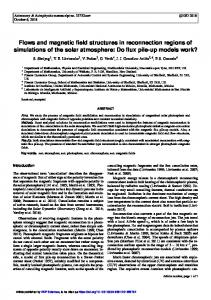
Magnetic field reconnection is defined as the process that occurs when magnetized plasmas with different magnetic field orientations flow together to alter the connectivity of the magnetic field. It occurs on spatial scales of the electron and ion skin depths (c/ωpe and c/ωpi, where ωpe and ωpi are the ion and electron plasma frequencies, respectively), after which accelerated plasma expands into a larger region where it may be further modified or accelerated by processes that are beyond the scope of the present discussion. We begin with the physical picture of Fig. 1, which depicts a region a few ion skin depths (~100 km at the sub-solar magnetopause) in size. The plasma that fills the figure is a two component neutral fluid that is bounded by magnetic field lines that are up on the right side and down on the left side of the figure, and for which, in each case, there is an electric field, Eo, out of the plane of the figure. Thus, the plasma on both sides of the figure EoxB/B2 drifts towards the center of the figure. The two oppositely directed magnetic fields may be unequal in magnitude or a magnetic field component, called the guide field, may exist out of the plane of Fig. 1. These features add complexity to the geometry without adding or deleting any physical principles from the fundamental processes that occur inside a few ion skin depths, so the guide field is assumed to be zero and the oppositely directed magnetic fields are assumed to be equal in magnitude. Fig. 1 describes the boundary

Figure 1 This would be the case for a closed terrestrial magnetosphere in which the solar wind plasma flows around the obstacle much as water flows around a rock in a stream. On the other hand, if the tangential electric field is non-zero, the plasmas continue flowing towards each other into the central region of the figure and magnetic field reconnection occurs as discussed below. The main effort in theoretical reconnection research has been the search for a large value of the tangential electric field in the central region (Parker, 1957; Parker,

1

1963; Sonnerup, 1981; Birn et al, 2001; Shay et al, 2001). Because this research is beyond the scope of this article, it is assumed that the tangential electric field in the central region is equal to Eo. Why has there been so much theoretical interest in making Eo large? Consider the current out of the plane in the central region of Fig.1, which is required by the curl of the magnetic field. A non-zero electric field results in a positive value of j·E in the central region of the figure and conversion of electromagnetic energy into particle energy, which is what magnetic field reconnection is all about. Where does the energy associated with this positive j·E originate? To answer this question, an analogy will be made with the electric circuit of Fig. 2, consisting of a battery and a resistor. From freshman physics, the electromagnetic energy conversion rate is VI where V is the battery voltage and I is the current. A second method for computing the energy conversion is to integrate j·E over the resistor volume. With j integrated over πr2, the cross-sectional area of the resistor, to give I and E integrated over the length of the resistor to become the potential drop V, the energy conversion rate is again VI. A third method is to consider the integral of the Poynting flux through the surface, S, that surrounds the resistor. Because E is everywhere along the axis of the cylinder and B everywhere circles the resistor, the Poynting flux, ExB/μo, is everywhere inward and its integrated magnitude is Eh(2πrB)/μo). Because Eh = V and 2πrB/μo = I, the result is again VI. A fourth way to compute the power dissipation is to utilize a later proof in this paper to say that magnetic field lines carry energy density B2/μo into the resistor at the ExB/B2 velocity, where the magnetic field is annihilated. This field line motion inserts (B2/μo)(E/B) or EB/μo units of energy per unit area per second, which is the same power input as given by the Poynting flux, so the answer is again VI.

Figure 2 Where does the converted electromagnetic energy go? It accelerates the plasma in the central region of Fig. 1 just as the resistor in Fig. 2 warms up due to energy conversion from the battery. The particle energy gain in Fig. 1 may be computed in a static model of a single ion species as follows. Consider a closed surface that extends between the two magnetic field lines of Fig. 1 and that has a length, h, along the field lines and a width, w, perpendicular to the plane of the figure. There is a net Poynting flux, 2whEoB/μo, through this surface from the right and the left. The number of particles that move into this volume per second at the EoxB/B2 velocity is 2whnEo/B, where n is the plasma density. Thus, the energy gained per particle is (2whEoB/μo)/( 2whnEo/B)=B2/nμo, and the average velocity increase of a low energy ion is v = [2B2/mnμo]1/2, where m is the ion mass. Thus, within a numerical factor ~1, the bulk flow of low energy ions is increased to the Alfven speed after reconnection. This has many consequences: •

If the EMF (in the case of Fig.2, a battery) is constant, the energy conversion rate is constant. This is analogous to the case of steady state reconnection at the dayside magnetopause, where the energy is continuously supplied by the solar wind that slows down. In both cases, the partial derivatives of all fields with respect to time are zero, so it is confusing to think of this process as magnetic field annihilation. This is just one example of problems arising from misinterpretation of the concept of moving magnetic field lines.

•

2

The flux, not the energy, of the ions emerging from the diffusion region increases with the increasing magnitude of the reconnection electric field, Eo. The ion energy is limited to that associated with the Alfven speed which, for typical parameters at the sub-solar reconnection region is ~1 keV. The electron bulk speed is also increased to the ion Alfven speed to maintain neutrality in the absence of an outgoing current. However, the electron energy is about 1/2000 of the ion energy because of the mass ratio. Thus, electrons are much less accelerated than the ions by reconnection in the diffusion region.

•

in the central region, the magnetic field lines in the central region must curve such that they tend to be perpendicular to the flow contours of Fig. 3. There are two approaches for obtaining a more quantitative picture of the magnetic field geometry. They are:

Although the energies of particles leaving the diffusion region are less than those observed in space, such particles may be accelerated further after leaving the diffusion regions. This acceleration may utilize the particle energy resulting from reconnection (Birn and Hesse, 2005) or it may use additional energy sources and mechanisms, such as are available by surfing on plasma waves, particles following meandering orbits, etc.

1. 2.

What happens to the plasma that is accelerated by the electromagnetic energy conversion? It must leave the central region by either flowing up/down or into/out of the plane of Fig. 1. A convenient simplification results from assuming that reconnection is a two-dimensional process, from which it follows that the plasma exits the central region of Fig. 1 in the vertical direction. It is not necessary that the geometry be twodimensional and in the real world it isn’t (Mozer et al, 2003b), although the current, j, flowing out of the plane of Fig. 1 suggests a tendency for a twodimensional geometry. To keep the geometry simple without losing any physics, it is assumed in this discussion that the plasma exits the central region by flowing vertically. This leads to bulk plasma flows like those indicated by the heavy lines in Fig. 3.

Solve Maxwell’s equations. Utilize a method of visualizing the magnetic field geometry without solving Maxwell’s equations. One such method is to assume that the magnetic field evolves in time by magnetic field lines moving at the ExB/B2 velocity.

Method 2 is preferable to method 1 as long as method 2 gives the same solution as method 1. If it does not, there is nothing magic about the situation. It is just that Maxwell’s equations must be solved in order to determine the magnetic field. In the following discussion, a condition is found under which the magnetic field geometry obtained by assuming that field lines move with ExB/B2 is the same as that produced by Maxwell’s equations (Longmire, 1963). The concept of moving magnetic field lines implies that field lines do not just pop up in a region of increasing magnetic field, but that the increasing field is associated with field lines flowing into that region from elsewhere. Because magnetic field lines are conserved in this picture, they obey a continuity equation which, in a coordinate system with the local magnetic field in the Z-direction, is δBZ/δt + ·(Bv) = 0 B

(1)

Selecting the field line velocity to be v=ExB/B2, the components of Bv are (Bv)X=EY and (Bv)Y=–EX, so equation 1 becomes δBZ/δt + δEY/δx – δEx/δy = 0 B

(2)

Figure 3

which is the z-component of Faraday’s law. Thus, without approximation and in the presence or absence of plasma, the magnitude of the magnetic field evolves as is required by Maxwell’s equations if magnetic field lines move with the ExB/B2 velocity. It is noted that any velocity v' satisfying ·(Bv')=0 may be added to ExB/B2 without modifying equation 1. Thus, there are an infinite number of magnetic field line velocities that preserve the magnitude of the magnetic field.

What is the magnetic field geometry associated with the flows of Fig. 3? Because the plasma flow is perpendicular to B, at least initially

The direction of a field line moving with ExB/B2 must also be the same as that obtained from Maxwell’s equations. To find the condition under

3

which this is true, consider two surfaces, S1 and S2 in Fig. 4, that are perpendicular to the field at times t and t + δt. At time t, a magnetic field line intersects the two surfaces at points a and b. Thus, the vector (b – a) is parallel to B(t). At the later time, t + δt, point a has moved along S1 at velocity ExB/B2(a) to point a' and it is on the illustrated magnetic field line. Meanwhile, point b has moved along S2 to b' at velocity ExB/B2(b) and it may or may not be on the field line that passes through a'. The question is, what are the constraints on these motions that result in a' and b' being on the same magnetic field line, i.e., that result in (b' - a') being parallel to B(t+δt)?

its cross product with B is zero. Because Bx(ExB/B2)=E−E|| and δB/δt=− xE, equation 6 is Bx( xE||) = 0

(7)

The vector (b'−a')=(b−a)+(b'−b)−(a'−a). The terms on the right side of this equation are: (b−a)=εB, because (b−a) is parallel to B. (a'−a)=[ExB/B2(a)] δt

Figure 4

2

(b'−b)=[ExB/B (b)]δt =[ExB/B2(a)+(b−a)δ(ExB/B2(a)/δr)]δt =[ExB/B2(a)+εB· (ExB/B2(a))]δt

This is the condition that preserves the direction of the magnetic field during its ExB/B2 motion. In most cases it requires that the parallel electric field be zero in order that field lines moving with ExB/B2 produce the same time evolution of the magnetic field as do Maxwell’s equations.

where r is a distance along the magnetic field line at time t. Combining terms gives 2

(b'−a')/ε = B+B· (ExB/B )δt

The existence and/or properties of plasma did not enter into the equation 7 requirement that field line motion at ExB/B2 produces the same result as Maxwell’s equations. Thus, field line motion does not require the presence of plasma, contrary to what some discussions of field line motion assume.

(3)

Also B'=B(a,t+δt) =B+(δB/δt)δt+(ExB/B2)· )Bδt

(4)

A vacuum example in which field line motion does not produce the same result as Maxwell’s equations occurs for a magnetic dipole placed in a uniform electric field, with the dipole axis parallel to the electric field direction (Falthammer, private communication). The ExB/B2 direction on a magnetic field line in the northern hemisphere is opposite to that on the same field line in the southern hemisphere, so the magnetic field lines appear to twist. This result is different from the solution to Maxwell’s equations for a dipole magnetic field, so something is wrong. In fact, Bx( xE||) ≠ 0 everywhere, so it is not possible to determine the magnetic field evolution by assuming that magnetic field lines move with the ExB/B2 velocity. There is nothing mysterious about this problem. It is just that the magnetic field must be

The problem reduces to finding the constraints that are imposed by the requirement that the right sides of equations 3 and 4 have a zero cross-product. To first order in δt, this gives Bx[δB/δt+(ExB/B2)· )B−B· (ExB/B2)]=0 (5) Using the vector identity for xMxN, for any two vectors M and N, allows rewriting equation (5) as Bx{δB/δt+ x(Bx(ExB/B2))+ B( ·(ExB/B2)–(ExB/B2) ·B}=0

(6)

The last term on the right is zero because ·B=0 and the next to last term may be neglected because

4

obtained from Maxwell’s equations and not from moving field lines.

region to magnetic field lines that were in the left input flow region. This is the change of magnetic field connectivity that is required by the earlier definition of magnetic field reconnection.

In the assumed absence of a parallel electric field in Fig. 3, the magnetic field evolution can be determined by moving a pair of magnetic field lines with the ExB/B2 velocity. This produces the magnetic field geometry of Fig. 5, which may be thought of as a superposition of snapshots at times t1,···· t5 of two magnetic field lines that ExB/B2 towards each other. There is the obvious problem that the magnetic field lines in the center of the plot have passed over each other to produce points having the magnetic field in two directions. This violation of Maxwell’s equations means that there must be a parallel electric field in the central region such that the magnetic field evolution in this region cannot be obtained by any means other than solving Maxwell’s equations. There is nothing magic about the central region, but only that one cannot obtain the magnetic field geometry in this region by moving magnetic field lines.

The only use of the concept of moving magnetic field lines in the above discussion has been to aid in determining the magnetic field configuration. If more than this use is made of moving field lines, there is a risk of drawing erroneous conclusions such as, because the magnetic field lines move in Fig. 6, δB/δt is non-zero. This is incorrect.

Figure 6.

Figure 5 Eliminating the magnetic field lines in the region having a parallel electric field leaves the geometry of Fig. 6. The reader is reminded that Fig. 6 shows the ion diffusion region while the interior of the dashed box will be shown to contain one or more electron diffusion regions.

Figure 7 The change of magnetic field connectivity in terrestrial reconnection is illustrated in Fig. 7. This figure shows three differently connected regimes, type 1 which contains magnetic field lines that go through the sun without going through the earth, type 2 which go through the earth without going

From the geometry of Fig. 6, magnetic field lines to the right of the figure in the input flow region have become connected in the outflow

5

through the sun and type 3 which go through both the earth and the sun. These topological boundaries are shown as the dashed X-line in Fig. 8. The discussion thus far has unanswered questions. For example: • • •

left

the left side of equation 10 or 11 must be non-zero. Because the jxB force of equation 10 acts on ions and because the ion inertial length, c/ωpi, and the ion gyroradius are much larger than the electron inertial length, c/ωpe, and the electron gyroradius, the ion bulk motion deviates from ExB/B2 on the larger spatial scale, called the ion diffusion region. Meanwhile, the electrons must ExB/B2 flow perpendicular to the plane of Fig. 8 and into the figure to produce the required j. This requires an electric field, En, perpendicular to the magnetic field and pointing towards the center of Fig. 8 from both sides in the ion diffusion region.

many

How do the ions and electrons move to create the current, j? How are the ions accelerated to the Alfven speed? How is the parallel electric field in the central region generated?

These questions will all be discussed through application of the Generalized Ohm’s Law as derived from the two-fluid equations of motion for a unit volume of plasma, which are (Spitzer, 1956): For ions nimi[δUi/δt+(Ui· )Ui] = niZe(E+UixB)– ·Pi+Pie

(8)

For electrons neme[δUe/δt+(Ue· )Ue] = –nee(E+UexB)– ·Pe+Pei

(9)

where • Ui and Ue are the ion and electron velocities averaged over unit volumes • ni and mi are the ion density and mass, respectively • ne and me are the electron density and mass, respectively • Pi and Pe are the ion and electron pressure tensors • Pie and Pei are the momentum transferred to ions (electrons) from electrons (ions) per unit volume per unit time. Subtraction of (9) from (8) assuming: • Neglect of quadratic terms • Electrical neutrality • Ignoring me/mi terms gives the Generalized Ohm’s Law E+UixB=jxB/en− ·Pe/en+(me/ne2)δj/δt+ηj

Figure 8 Ions entering from the left or right are accelerated by En and the jxB force to the opposite side of the central region where they are decelerated, turned around, and again accelerated. They bounce between the two sides to eventually exit vertically at the Alfven speed. Because enEn≈jB according to equation 10, and because the sum of the two forces times the distance c/ωpi is about equal to the energy B2/μo gained by a unit volume of fluid, the electric field is En≈valfvenB/2. This is ~20 mV/m at the sub-solar magnetopause. This electric field and the associated ion counterstreaming and acceleration have been observed in space (Mozer et al, 2002; Wygant et al, 2005). It is also important to note that the ions are accelerated in a region having the ion scale and not in the much smaller electron diffusion region that is discussed below.

(10)

where η is the Coulomb or anomalous resistivity. Equivalently, because j/ne = Ui − Ue, E+UexB=− ·Pe/en+(me/ne2)δj/δt+ηj

(11)

For the current, j, to exist out of the plane of Fig. 8 the ions and electrons must move differently, i.e.,

6

The electric field, En, existing along the dashed X in Fig. 8 over a scale size of c/ωpi, has a non-zero divergence so it must result from charge separation. This requires that electrons move along the magnetic field lines into the dashed box to create the charge separation. The parallel (to B) electric field in the dashed box accelerates these electrons to the outgoing ion bulk velocity, after which they are ejected into the upper and lower central regions. Thus, the average parallel electric field in the dashed box must be downward (upward) in the upper (lower) part of the dashed box. This in-plane electron current causes the outof-plane quadrupolar magnetic field that is illustrated in Fig. 8 and that has been observed in space (Mozer et al, 2002) and in the lab (Ren et al, 2005). The jxB/en term in equation 10, the quadrupolar magnetic field, and the bipolar electric field constitute the essence of Hall MHD reconnection physics.

should not be obtained from cartoons, it is important to consider that the dashed box may contain a large number of electron scale structures, each of which is located where the magnetic field is non-zero and each of which contains a parallel electric field. This possibility is strongly supported by both computer simulations (Onofri et al, 2004; Daughton, private communication, 2006) and experimental data (Mozer, 2005). The reconnection rate is proportional to the number of magnetic field lines crossing into the reconnection region per unit area per second. Because the density of field lines is B and their velocity is EoxB/B2, the rate of field line entry is the density times the velocity, or Eo. This is why the tangential electric field is sometimes referred to as the reconnection rate.

What is the nature of the parallel electric field inside the dashed box of Fig. 8? The right side of equation 11 must differ from zero in this region because of the parallel electric field on the left side. Thus, the parallel electric field must be associated with the time derivative of j (inertial effects), the divergence of the pressure tensor, or finite resistivity. Experimental data suggests that it is associated with the pressure tensor (Mozer et al, 2002; Mozer, 2005), but this is an important issue that remains to be fully resolved. At any rate, because of the additional terms in equation 11, electrons do not move with the ExB/B2 velocity, so they are said to be unmagnetized in the electron diffusion region..

What does sub-solar reconnection do for magnetospheric physics? Because the ions and electrons are accelerated only to the Alfven speed and because most of this accelerated plasma escapes into the solar wind, it may appear that dayside reconnection is not important. This conclusion is incorrect because reconnection also modifies the magnetic field connectivity to produce a long tail in the anti-sunward direction, as illustrated in Fig. 7. In the southern hemisphere tail, the magnetic field points away from the earth and in the northern hemisphere tail, it points earthward. In the presence of a dawn-to-dusk electric field, the Poynting vector along the tail surface is everywhere inward, so its integral over this surface provides an energy source for driving magnetospheric processes. For a tail that is 300 earth radii in length and 30 earth radii in diameter, the energy input associated with a magnetic field of 10 nT and a cross-tail electric field of 0.5 mV/m is ~2x1012 watts. This is more than sufficient to drive all known magnetospheric processes and it is more than four orders-of-magnitude larger than the energy directly available from sub-solar reconnection. The EMF that provides this energy is the kinetic energy of the solar wind, which slows as it moves along the tail.

The scale size for which the terms on the right side of equation 11 become important is ~c/ωpe (Vasyliunas, 1975). A single region of this size is frequently drawn at the crossing of the dashed X in Fig. 8 to represent the electron diffusion region. From such a cartoon, it is sometimes incorrectly concluded that the magnetic field must be zero and the plasma beta must be large in the electron diffusion region. Because physical conclusions

For the sub-solar region, it may seem that the reconnection rate need only be large enough to produce the long tail. However, a large Poynting flux into the tail implies a large ExB/B2 flow of magnetic field lines into the tail and these field lines must also reconnect. Because the average reconnection on the dayside and in the tail must be equal, a large Poynting flux into the tail must be accompanied by a large sub-solar reconnection rate.

It is important to note that less than 1% of satellite sub-solar magnetopause crossings exhibit clear signatures of the quadrupolar magnetic field and bipolar electric field of Fig. 8 (Mozer et al, 2002). This is undoubtedly due to time variations, real geometries that differ from the idealized twodimensional geometry of equal and opposite magnetic fields, spacecraft crossings at distances far from the center of the reconnection region, etc.

7

In summary, topics for future research on magnetic field reconnection include: •

• • • •

Mozer, F.S., J. Geophys. Res., (1005), 110(A12), A12222 Mozer, F.S., S.D. Bale, J.P. McFadden, and R.B. Torbert (2005), New features of electron diffusion regions observed at sub-solar magnetic field reconnection sites, Geophys. Res. Lett., 32(24), L24102 Mozer, F.S., H. Mitsui, and R.B. Torbert (2006), Electron scale structures are everywhere: Are they electron diffusion regions? EGU, Vienna Onofri, M., L. Primavera, F. Malara, and P. Veltri (2004) Three-dimensional simulations of magnetic reconnection in slab geometry, Phys. Plasmas, 11 Parker, E.N. (1957), Sweet’s mechanism for merging magnetic fields in conducting fluids, J. Geophys. Res., 62, 509. Parker, E.N. (1963), The solar flare phenomenon and the theory of reconnection and annihilation of magnetic fields, Ap. J. Suppl., 8, 177. Ren, Y., M. Yamada, H. Ji, S.P. Gerhardt, R. Kulsrud, and A. Kuritsyn (2005), Experimental verification of the Hall Effect during pull reconnection in MRX, Phys. Rev. Lett, 95, 055003. Shay, M.A., J.F. Drake, B.N. Rogers and R.E. Denton, (2001), Alfvenic collisionless magnetic reconnection and the Hall term, J. Geophys. Res., 106, 3759 Sonnerup, B.U.O., et al. (1984), Reconnection of magnetic fields, in Solar Terrestrial Physics: Present and Future, NASA Ref. Pub. 1120, edited by D.M. Butler and K. Papadapolous. Spitzer, L. Jr. (1956), Physics of fully ionized gases, Interscience tracts on physics and astronomy, Editor R.E. Marshak, Interscience Publishers, Inc., New York. Vasyliunas, V.M. (1975), Theoretical models of magnetic field line merging, Rev. Geophys. Space Phys., 13, 303. Wygant, J.R., C. A. Cattell, R. Lysak, Y. Song, J. Dombeck, J. McFadden, F. S. Mozer, C. W. Carlson, G. Parks, E. A. Lucek, A. Balogh, M. Andre, H. Reme, M. Hesse, and C. Mouikis, (2005), Cluster observations of an intense normal component of the electric field at a thin reconnecting current sheet in the tail and its role in the shock-like acceleration of the ion fluid into the separatrix region, J. Geophys. Res., 110, A09206, doi:10.1029/2004JA010708

Microphysics in the electron diffusion region. Understanding the relative importance of inertial effects, resistivity, and the gradient of the pressure tensor. Processes that result from the reconnection geometry and that accelerate ions and electrons to high energies on short time scales. Wave modes associated with reconnection and the subsequent particle acceleration. The mechanism for generating parallel electric fields in the electron diffusion region. The importance of electron diffusion regions that are observed throughout the magnetopause as well as in the magnetosphere, the magnetosheath, and the bow shock (Mozer et al, 2006).

ACKNOWLDEGEMENTS The author thanks C.-G. Falthammar for many helpful discussions over many years, and his Berkeley colleagues for many helpful comments. This work was supported by NASA Grants NNG05GC72G and NNG05GL27G. REFERENCES Birn, J., J.F. Drake, M.A. Shay, B.N. Rogers, R.E. Denton, M. Hesse, M. Kuznetsova, Z.W. Ma, A. Bhattacharjee, A. Otto, and P.L. Pritchett (2001), Geospace environmental modeling (GEM) magnetic reconnection challenge, J. Geophys. Res., 106, 3715. Birn, J. and M. Hesse (2005), Energy release and conversion by reconnection in the magnetotail, Ann. Geophys., 23, 3365 Longmire, C.L. (1963), Elementary plasma physics, Interscience Publishers, John Wiley and Sons, New York. Mozer, F.S., S.D. Bale, and T.D. Phan (2002), Evidence of diffusion regions at a sub-solar magnetopause crossing, Phys. Rev. Lett., 89, 015002, doi: 10.1103/PhysRevLett.89.015002. Mozer, F.S., S.D. Bale, T.D. Phan, and J.A. Osborne (2003a), Observations of electron diffusion regions at the subsolar magnetopause, Phys. Rev. Lett., 91, 245002. Mozer, F.S. T.D. Phan, and S.D. Bale (2003b), The complex structure of the reconnecting magnetopause, Phys. Plasmas, 10, 2480. Mozer, F.S., S.D. Bale, J.D. Scudder, (2004), Geophys. Res. Lett., 31, L15802

8