Color-Shape Context for Object Recognition - CiteSeerX

JOURNAL OF LATEX CLASS FILES, VOL. 1, NO. 11, NOVEMBER 2002

1

Color-Shape Context for Object Recognition Aristeidis Diplaros, Student Member, IEEE, Theo Gevers, Member, IEEE, and Ioannis Patras, Member, IEEE,

A BSTRACT We propose a new image feature that merges color and shape information. This global feature, which we call color shape context, is a histogram that combines the spatial (shape) and color information of the image in one compact representation. This histogram codes the locality of color transitions in an image. Illumination invariant derivatives are first computed and provide the edges of the image, which is the shape information of our feature. These edges are used to obtain similarity (rigid) invariant shape descriptors. The color transitions that take place on the edges are coded in an illumination invariant way and are used as the color information. The color and shape information are combined in one multidimensional vector. The matching function of this feature is a metric and allows for existing indexing methods such as R-trees to be used for fast and efficient retrieval. K EYWORDS : Photometric and geometric invariants, color-shape context, image retrieval, object recognition. I. I NTRODUCTION Theo: object recognition introduction Over the last decade, the amount of visual information (images and video) on the Internet is growing exponentially. This large and continually growing amount of images on the Internet calls for contend-based image retrieval (CBIR) frameworks. Many CBIR systems have been developed describing the image content by low-level features (e.g. color, shape, texture) and/or high-level features (e.g. faces, trees). Usually the highlevel features are not as general as the low-level features, but are more domain specific in the sense that they are designed to detect a special class of images or objects. Further, in general, high-level features include training which is done usually done by manually selecting representative images. However, in most of the CBIR-systems, color and shape information is treated separately. It is our opinion that color and shape information should be used together to augment the performance of image retrieval. Many CBIR systems have been developed in the recent years which try to describe the image content using a combination of low-level features and/or high-level features [26]. The high-level features are often calculated from the low-level features. Usually the high-level features are not as general as the low-level features, but are instead domain specific in the sense that they are designed to detect a special complex class of images or objects, (e.g. faces, trees) and require training bla-bla is with the ISIS.

using manually selected representative images. The high-level features are therefore divided into general and domain specific features [28]. Still, the world of CBIR is dominated by systems that utilize low level features. Indeed, the generality of such features make them particularly applicable for describing the appearance of wide variety of objects. The challenges lie in deriving the features that describe sufficiently well the objects even when captured from a variety of viewpoints, under different illumination conditions and under occlusions or clutter. For achieving this goals, color, shape and texture features have been extensively used independently from one another in a number of retrieval systems. However, more and more it becomes apparent that their combinations may provide features with much higher discriminative power than each one separately [27]. Therefore, in this paper, we study computational models and techniques to merge color and shape invariant information for CBIR. Shape deformations occur by a change in viewpoint, object position etc. Deformations for the color channels occur due to shading, illumination, shadows etc. To this end, a vector-based framework is used to index images on the basis of color, shape and composite information. The scheme makes use of a color-shape context providing a high-discriminative cue in vector form to be used as an index. The paper is organized as follows. First, we propose a scheme to compute illumination invariant derivatives in a robust way. Then, shape invariance is discussed in Section III. In Section IV, we present a framework to combine and match color and shape invariant information. Finally, experiments are given in Section V. Theo: CBIR introduction In a general context, object recognition involves the task of identifying a correspondence between a 3-D object and some part of a 2-D image taken from an arbitrary viewpoint in a cluttered real-world scene. Many practical object recognition systems are appearanceor model-based. To succeed they address two major interrelated problems: object representation and object matching. The representation should be good enough to allow for reliable and efficient matching. The recognition consists of matching the stored models (model-based) or images (appearance-based), encapsulated in a representation scheme, against the target image to determine which model (image) corresponds to which portion of the target image. Several systems have been developed to deal with the problem of model-based object recognition by solving the correspondence problem by tree search. However, the computational complexity is exponential for nontrivial images. Therefore, in this paper, we focus on appearance-based object recognition.


Most of the work on appearance-based object recognition based on shape information is by matching sets of shape image features (e.g. edges, corners and lines) between a query and a target image. In fact, the projective invariance of cross ratios and its generalization to cross ratios of areas of triangles and volumes of tetrahedra has been used for viewpoint invariant object recognition and significant progress has been achieved [22]. Other shape invariants are computed based on moments, Fourier transform coefficients, edge curvature and arc length [21], [25]. Unfortunately, shape features are rarely adequate for discriminatory object recognition of 3-D objects from arbitrary viewpoints. The shape-based approach is often insufficient especially in case of large data sets [12]. Another way to appearance-based object recognition is to use color (reflectance) information. It is well known that color provides powerful information for object recognition, even in the total absence of shape information. A common recognition scheme is to represent and match images on the basis of color invariant histograms [19], [10]. The color-based matching approach is widely in use in various areas such as object recognition, content-based image retrieval and video analysis. Little research has been done on how to combine color and shape information for object recognition. Important work is done by [5], [15] using moment invariants that combine geometric and photometric changes for planar objects. Further, in [12] color and shape invariants are combined for object recognition based on geometric algebraic invariants computed from color co-occurrences. Although the method is efficient and robust, the discriminative power decreases by the amount of invariance. Color, shape and texture are combined in [14] for visual object recognition. However, the scheme is heavily dependent on severe illumination changes. Therefore, in this paper, we study computational models and techniques to merge color and shape invariant information to recognize objects in 3D- scenes. Shape deformations occur by a change in viewpoint, object position etc. Deformations for the color channels occur due to shading, illumination, shadows etc. To this end, a vector-based framework is used to index images on the basis of color, shape and composite information. The scheme makes use of a color-shape context providing a high-discriminative cue in vector form to be used as an index. In this paper we do not consider robustness against cluttering and occlusion. The recognition scheme is designed according to the following principles: 1. Generality: the class of objects from which the images are taken from is the class of multicolored planar objects in 3-D real-world scenes. 2. Invariance: the scheme should be able to deal with images obtained from arbitrary unknown viewpoints discounting deformations of the shape (viewpoint, object pose) and color (shadowing, shading and illumination). 3. Stability: the scheme should be robust against substantial sensing and measurement noise. The paper is organized as follows. First, we propose a scheme to compute illumination invariant derivatives in a robust way. Then, shape invariance is discussed in Section III. In Section IV, color and shape invariant information is combined. Matching is discussed in Section IV-B. Finally, experiments are given in Section V.

2

II. P HOTOMETRIC I NVARIANTS FOR C OLOR I MAGES The color of an object varies with changes in illuminant color (Spectral Power Distribution) and geometry (i.e. angle of incidence and reflectance). Hence, in outdoor images, the color of the illuminant (i.e. daylight) varies with the time-of-day, cloud cover and other atmospheric conditions. Consequently, the color of an object may change drastically due to varying imaging conditions. A. Illumination Invariant Derivatives Various illumination-independent color ratios have been proposed [10], [16]. These color ratios are derived from neighboring points. A drawback, however, is that these color ratios might be negatively affected by the geometry and pose of the object. Therefore, we focus on the following color ratio [11]: M (C~x11 , C~x12 , C~x21 , C~x22 ) =

C~x11 C~x22 1 , C 6= C 2 , C~x12 C~x21

(1)

expressing the color ratio between two neighboring image locations, for C 1 , C 2 ∈ {C 1 , C 2 , ..., C N } giving the measured sensor pulse response at different wavelengths, where ~x1 and ~x2 denote the image locations of the two neighboring pixels. For a standard RGB color camera, we have: R~x1 G~x2 m1 (R~x1 , R~x2 , G~x1 , G~x2 ) = , (2) R~x2 G~x1 m2 (R~x1 , R~x2 , B~x1 , B~x2 ) =

R~x1 B~x2 , R~x2 B~x1

(3)

m3 (G~x1 , G~x2 , B~x1 , B~x2 ) =

G~x1 B~x2 . G~x2 B~x1

(4)

The color ratio is independent of the illumination, a change in viewpoint, and object geometry [11]. For the ease of exposition, we concentrate on m1 based on the RG-color bands in the following discussion. Without loss of generality, all results derived for m1 will also hold for m2 and m3 . Taking the natural logarithm of both sides of Eq. 2 results for m1 in: ln m1 (R~x1 , R~x2 , G~x1 , G~x2 ) = ln(

R~x1 G~x2 )= R~x2 G~x1

R~x2 R~x1 ) − ln( ) ~ x G 1 G~x2 (5) Hence, the color ratios can be seen as differences at two neighboring locations ~x1 and ~x2 in the image domain of the logarithm of R/G: ln R~x1 + ln G~x2 − ln R~x2 − ln G~x1 = ln(

R R ~x1 )) − (ln( ))~x2 (6) G G By taking these differences in a particular direction between neighboring pixels, the finite-difference differentiation is obtained of the logarithm of image R/G which is independent of the illumination color, and also a change in viewpoint, the object geometry, and illumination intensity. We have taken the gradient magnitude by applying Canny’s edge detector ∇m1 (~x1 , ~x2 ) = (ln(


(derivative of the Gaussian with σ = 1.0) on image ln(R/G) with non-maximum suppression in a standard way to obtain gradient magnitudes at local edge maxima denoted by Gm1 (~x), where the Gaussian smoothing suppresses the sensitivity of the color ratios to noise. The results obtained so far for m1 hold also for m2 and m3 , yielding a 3-tuple (Gm1 (~x), Gm2 (~x), Gm3 (~x)) denoting gradient magnitude at local edge maxima in images ln(R/G), ln(R/B) and ln(G/B) respectively. For pixels on a uniformly colored region (i.e. with fixed surface albedo), in theory, all three components will be zero whereas at least one the three components will be non-zero for pixels on locations where two regions of distinct surface albedo meet. Higher order derivatives are taken to obtain salient points such as corners and T-junctions. These higher order derivatives are computed again by Gaussian derivatives applied on the illumination invariant color model. For the ease of exposition we concentrate on ln m1 in the following discussion. To compute higher order derivatives, we apply the partial R derivatives of the Gaussian up to order 2 for image ln G . Let {∇m1x , ∇m1y , ∇m1xx , ∇m1yy , ∇m1xy }σ denote the set of the first five partial Gaussian derivatives. From these partial derivatives, we have computed the Laplacian and the Hessian. Note that the Laplacian operator finds its roots in the modeling of certain psychophysical processes in mammalian vision and hence is suited to compute ’visual salient’ points. B. Noise Robustness of Illumination Invariant Derivatives The above defined illumination derivatives may become unstable when intensity is low. In fact, these derivatives are undefined at the black point (R = G = B = 0) and they become very unstable at this singularity, where a small perturbation in the RGB-values (e.g. due to noise) will cause a large jump in the transformed values. As a consequence, false color constant derivatives are introduced due to sensor noise. These false gradients can be eliminated by determining a threshold value corresponding to the minimum acceptable gradient modulus. We aim at providing a method to determine automatically this threshold by computing the uncertainty for the color constant gradients through noise propagation as follows. Additive Gaussian noise is widely used to model thermal noise and is the limiting behavior of photon counting noise and film grain noise. Therefore, in this paper, we assume that sensor noise is normally distributed. Then, for an indirect measurement, the true value of a measurand u is related to its N arguments, denoted by uj , as follows u = q(u1 , u2 , · · · , uN ) (7) Assume that the estimate u ˆ of the measurand u can be obtained by substitution of u ˆj for uj . Then, when u ˆ1 , · · · , u ˆN are measured with corresponding standard deviations σuˆ1 , · · · , σuˆN , we obtain [20] u ˆ = q(ˆ u1 , · · · , u ˆN ). (8) Then, it follows that if the uncertainties in u ˆ1 , · · · , u ˆN are independent, random and relatively small, the predicted un-

3

certainty in q is given by [20] v uN uX ∂q σuˆi )2 σq = t ( ∂ u ˆ i j=1

(9)

the so-called squares-root sum method. Although (9) is deduced for random errors, it is used as an universal formula for various kinds of errors. Focusing on the first derivative, the substitution of (6) in (9) gives the uncertainty for the illumination invariant coordinates v u 2 2 2 2 u σR~x σG σR σG ~ x ~ x ~ x σ∇m1 (~x1 , ~x2 ) = t 2 1 + 2 1 + 2 2 + 2 2 R~x1 G~x1 R~x2 G~x2

(10)

Assuming normally distributed random quantities, the standard way to calculate the standard deviations σR , σG , and σB is to compute the mean and variance estimates derived from a homogeneously colored surface patches in an image under controlled imaging conditions. From the analytical study of Eq.10, it can be derived that color ratio becomes unstable around the black point R = G = B = 0. Further, to propagate the uncertainties from these color components through the Gaussian gradient modulus, the uncertainty in the gradient modulus is determined by convolving the confidence map with the Gaussian coefficients. As a consequence, we obtain: ¤ P £ i (∂ci /∂x) · σ∂ci /∂x + (∂ci /∂y) · σ∂ci /∂y pP σ∇F ≤ , (11) i [(∂ci /∂x) + (∂ci /∂y)] where i is the dimensionality of the color space and ci is the notation for particular color channels. In this way, the effect of measurement uncertainty due to noise is propagated through the color constant ratio gradient. For a Gaussian distribution 99% of the values fall within a 3σ margin. If a gradient modulus is detected which exceeds 3σ∇F , we assume that there is 1% chance that this gradient modulus corresponds to no color transition. III. G EOMETRIC I NVARIANT T RANSFORMATION In this section, shape transformations are discussed to measure shape properties of a set of coordinates (i.e. edges, corners and T-junctions) of an image object independent of a coordinate transformation. To this end, we consider the edges, computed from the illumination invariant derivatives proposed in previous section, as the spatial information which is normalized by the aspect ratio given in following Section. A. Affine Deformations and Inverse Transformation The geometric deformations considered in this paper are up to affine transformations: x~0 = A~x + B

(12)


4

where a point ~x = (x, y) in one image is transformed into the corresponding point x~0 = (x0 , y 0 ) in the second image, with transformation matrix: · ¸ · ¸ a11 a12 b1 A= ,B = (13) a21 a22 b2 This transformation is consider to approximate the projective transformation of 3-D planar objects , therefore is valid when the object is relative far away from the camera. It is known that the spatial moment is defined as: Mu (m, n) =

J X K X

(14)

(1,0) M (0,1) Further, the ratio’s xk = M M (0,0) , y k = M (0,0) define the centroid. Transforming the image with respect to b = T [xk y k ] yields invariance to translation. The principle axis is obtained by rotating the axis of the central moments until M11 is zero. Then, the angle θ between the original and the principle axis, is defined as follows [17]:

2M11 (15) M20 − M02 This angle may be computed with respect to the minor or the major principal axis. To determine the unique orientation,we require the additional condition that M20 > M02 and M30 = 0. Setting the rotation matrix to · ¸ cos θ − sin θ A= (16) sin θ cos θ tan 2θ =

will provide rotation invariance. A change in scale by a factor of δ in the x-direction and γ in the y-direction is given by 0

Mu (m, n) = δ m+1 γ n+1 Mu (m, n) where 0

0

Mu (0, 0) = Mu (0, 0) = 1 and Mu (2, 0) = Mu (0, 2) then we obtain δ = 1/γ where δ = (Mu (0, 2)/Mu (2, 0))0.25

A. Color-Shape Representation Scheme The color-shape framework is as follows. For a color image I : R2 → R3 , illumination invariant edges are computed to obtain a binary image E : R2 → {0, 1}. Then at the edge points we define: p~n = (x, y, m1 , m2 , m3 )| E(x, y) = 1

n xm k yj f (j, k)

j=1 k=1

0

to represent the distribution of quantized invariant values in a multidimensional invariant space. Color-shape contexts are formed on the basis of color, shape and combination of both.

(17)

In conclusion, we normalize our spatial information with respect to translation and rotation using a collection of loworder moments. The scale invariance and the robustness to affine transformation are discussed in the following section. IV. I NDEXING AND M ATCHING In this section, we propose an alternative indexing scheme to combine shape and color information. The scheme is called the color-shape context which is related to the shape context proposed by [1] for shape matching. The difference is that the color-shape context combines both color and spatial information into one unifying indexing framework. Moreover, the scheme is robust to affine deformations of shape and color. b Let the image database consist of a set {Id }N d=1 of color images. Color-shape contexts are created for each image Id

(18)

where x, y are pixel coordinates in image E and m1 , m2 , m3 are the color invariant ratios calculated in image I. Further, p~n ∈ R5 . We can decompose each of these p~n vectors as follows: p~n = p~Sn + p~Cn

(19)

where: p~Sn = (x, y, 0, 0, 0) p~Cn = (0, 0, m1 , m2 , m3 ) Note that the set P = {p1 , p2 , . . . , pn } of n points in a 5-dimensional space representing both the shape and color information in the image. Each of these n points is now considered to represent a vector originating from a central point. To provide noise robustness, we consider the distribution of these vectors over relative positions. Then, the color-shape context hcP of set P is defined as the coarse histogram of the distribution of all pn vectors, as defined in Eq.19, over the relative position c. In other words, the histogram of the decomposed and quantized versions of the pn vectors, with respect to the distance and orientation from a central point c, is called color-shape context of the image. The vector p~S is represented by its polar coordinates while the vector p~C is represented with its spherical coordinates. To construct the color-shape context of each image I using a relative position c, we first translate the vectors p~Sn with respect to point c and then the following histogram is computed: hcP (k) =

#{q : q ∈ bin(k)} n

(20)

where q ∈ P and bin(k) is a bin corresponding to a partition of the feature space. This bin is defined as a Cartesian product of the spatial and color bins. For partitioning the spatial space, we compute the log-polar with equally spaced radial bins. An equally-spaced bins scheme is used to partition the 3-D color invariant space. Note that the color-shape context feature is rotation, scale, translation and aspect ratio change invariant. Further, the colorshape context has intrinsic robustness against small amounts of displacement noise, since it is based on the distribution of illumination invariant derivatives instead of their exact positions. Total affine invariance, which would include skew invariance, is not claimed, but the experimental results show that the feature is robust to affine transformations.


5

B. Matching in simple scenes For object recognition in simple scenes (i.e. one object per image) we set the relative position c as the center of gravity of the spatial information. Note that the shape information is normalized and that the center of gravity is at the origin (0, 0). To achieve scale invariance we normalize all |~ pSn | with respect to the mean distance between all point pairs in E. Let’s consider an image a with corresponding color-shape P context ha . Because ha (k) ∈ [0, 1] and k ha (k) = 1, the cost function to compute the distance with another color-shape context hb is given by: K

Cab =

1 X (ha (k) − hb (k))2 2 (ha (k) + hb (k))

(21)

k=1

The complexity of this operation is only dependent on the number of K which is constant for all images in the database and is usually small. Note that the color-shape context feature is rotation, scale, translation and aspect ratio change invariant. Furthermore, the color-shape context exhibits intrinsic robustness against small amounts of displacement noise, since it is based on the distribution of illumination invariant derivatives instead of their exact positions. C. Matching in complex scenes For CBIR and object recognition in complex scenes, which may contain cluttering and occlusion, a modified matching strategy is adopted. The reason is that the framework based on moments, used to determine the center and the scale of the color-shape context, can no longer be used since the edge points may belong to more than one objects. In addition, occlusions and cluttering result in shape contexts that contain information about the background and/or the other objects in the scene. For these shape contexts, it is apparent that the influence of cells that contain such, irrelevant, information should be reduced in the matching scheme. To this end, we build multiple representations of color-shape context per image and match them with a modified distance function. The multiple color-shape contexts (in our CBIR experiments each image was described by 5 color-shape contexts) are build at specific image locations, same for all images. The scale and orientation of these color-shape contexts are fixed for all images in the dataset. The modification of the cost function aims at reducing the influence of large costs introduced at occlusions. More specifically, we introduce an occlusion field that indicates in which spatial cell occlusion occurs and modify the cost function in order to reduce the cost of matching when the occlusion fields are spatially coherent. More specifically, the occlusion field of spatial cell k is defined as: ½ 1 : dk /qk > T Ok = 0 : dk /qk ≤ T where dk denotes the accumulated cost of matching in the spatial cell k and is defined as : X (ha (n) − hb (n))2 1 dk = 2 (ha (n) + hb (n)) {n | f (n)=k}

where f(n) denotes a mapping from the index of the colorshape context to the appropriate spatial cell index k. qk denotes the percentage of points of the two images in the spatial cell k and is defined as: X qk = (ha (n) + hb (n)) {n | f (n)=k}

The cost function is now as follows: 0

Cab = Cab −

X k

Ok

1 X (dk − T qk Ol ) |Nk |

(22)

l∈Nk

where Nk is the 4-neighborhood of spatial cell k. The way that 0 Cab is defined is that it assigns a cost at the occluded spatial cell k that varies between qk T and dk depending on the spatial coherency of the occlusion fields in the neighborhood of k. In the extreme cases, if none of the l ∈ Nk is occluded the local cost at the spatial cell k is dk while if all l ∈ Nk are occluded it is qk T . V. E XPERIMENTS In this section, we consider the performance of the proposed method. Therefore, in section V-A, the datasets we used in our experiments are discussed. Then, in the remaining sections, we test our method on these three different datasets. We use two kinds of measures for our experiments: 1) For a measure of match quality to viewpoint changes and illumination robustness, let rank rQi denote the position of the correct match for test image Qi , i = 1, ..., N2 , in the ordered list of N1 match values. The rank rQi ranges from r = 1 from a perfect match to r = N1 for the worst possible match. Then, for one experiment with N2 test images, the average ranking percentile is defined as: r=(

N2 1 X N1 − rQi )100% N2 i=1 N1 − 1

(23)

2) To evaluate the effectiveness of the image retrieval, we compute: • Precision is the percentage of similar images retrieved with respect to the total number of retrieved images. • Recall is the percentage of similar images retrieved with respect to the total number of similar shapes in the dataset. b be the set of similar images in the Specifically, let A dataset, and let A denote the set of the retrieved images from the system. Precision p and recall r are then given as: T b

p = ( |A|A|A| )100% ,

T b

A| )100% r = ( |A|A| b

We will present precision-recall plots. The horizontal axis in such a plot corresponds to the measured recall while, the vertical axis corresponds to precision. Each method in such a plot is represented by a curve. Each


query retrieves the best 100 answers (best matches) and each point in our plots is the average over all queries. Precision and recall values are computed from each answer set after each answer (from 1 to 100) and, therefore, each plot contains exactly 100 points. The top-left point of a precision/recall curve corresponds to the precision/recall values for the best answer or best match (which has rank 1), while the bottom right point corresponds to the precision/recall values for the entire answer set. A method is better than another if it achieves better precision and better recall. This method is depicted as the one having its corresponding curve above the curves belonging to the other methods. The method achieving higher precision and recall for large answer sets is considered to be the better method (based on the assumption that typical users usually retrieve 10 to 20 images). A. The Datasets For comparison reasons, we have selected three different datasets: Amsterdam and Columbia - COIL-100, which are publicly available and often used in the context of object recognition [12], [23].

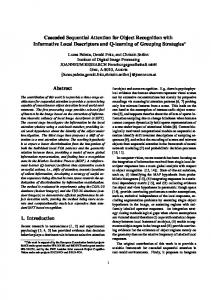
Fig. 1. Various images which are included in the Amsterdam image dataset of 500 images. The images are representative for the images in the dataset. Objects were recorded in isolation (one per image).

Amsterdam Dataset: In Fig. 1, various images from the image database are shown. These images are recorded by the SONY XC-003P CCD color camera and the Matrox Magic Color frame grabber. Two light sources of average day-light color are used to illuminate the objects in the scene. The database consists of N1 = 500 target images taken from colored objects, tools, toys, food cans, art artifacts etc. Objects were recorded in isolation (one per image). The size of the images are 256x256 with 8 bits per color. The images show a considerable amount of shadows, shading, and highlights. A second, independent set (the query set) of N2 = 70 query or test recordings was made of randomly chosen objects already in the database. These objects were recorded again one per image with a new, arbitrary position and orientation with respect to the camera, some recorded upside down, some rotated, some at different distances. COIL-100: In order to test the performance of our algorithm against variability in appearance, the COIL-100 has been selected which have been collected at the Columbia University [29]. For these experiments, we aim at multi-view object recognition i.e. there are various images taken from the object (i.e. back, front, from aside etc.), see Fig. 2. However, a number of objects in the database are single-colored and therefore hard to recognize.

6

COREL: For our CBIR experiments we used a subset of the Corel image collection. This subset consists of 25 categories and has a total of 2600 images. These categories cover a wide rage of subjects, which includes among others buildings, ships, mountains, cars, flowers and sunsets. This dataset can be considered as a representative collection of images found on the internet, since, it consists of photos taken by both amateurs and professionals in different conditions and with different equipments. In this dataset we randomly selected 10% of the images from every category to be the query set. This is a total of 260 queries. In order to establish a ground truth for our tests we consider all pictures that belong to a category to be relevant. Of course not all of the images in a category are visually similar but this choice facilitates automatic evaluation of the results. An alternative would be to use human subjects to define the ground truth, this would require, for each method, at least 20 human relevance judgments for each one of the 260 queries. B. Viewpoint Robustness To test the effect of change in viewpoint we used the COIL100 dataset. This dataset consist of 7200 images from 100 objects which have been put perpendicularly in front of the camera and in total 72 recordings were generated by varying the angle between the camera with 5 degrees with respect to the object, see Fig. 2. We conducted our experiment as following, we gave as a query a view of an object ranging from 0 to 70 degrees (15 different views) and the method had to recognize the corresponding object from the 0 degrees views of all 100 objects. This was done for all 100 objects and for all 15 views of each object. We concentrate on the quality

Fig. 2. Different images recorded from the same object under varying viewpoint. The COIL-100 database consisting of 7200 images of 100 different objects with 72 different views each.

of the recognition rate with respect to varying viewpoint differentiated by color information, shape information, and the integration of both. Therefore, we first study to what extent the proposed framework is viewpoint independent. In the mean time, we research on whether the combination of color and shape invariant information will outperform the matching scheme based on only color or shape. To this end, we have constructed three different color-shape context histograms. Firstly, we have included both color and shape invariant information denoted by HCS . Secondly, only color is considered which will be given by HC . Thirdly, we used only shape information denoted by HS . Also, we have included in our experiment the well-known, color-based method of Histogram Intersection [19] denoted by HI RGB . With HI inv−rgb we denote the results of the Histogram Intersection when the images have been initially transformed to the normalized rgb color space. The performance of the recognition scheme is given in Fig. 3. When the performance of different invariant


?b 4 + ×

90

r

? + × b 4

? + × b 4

Average ranking + + ? ? ? + ×b ×b b × 4 4 4 rH C

80

70

percentile r against rotation θ ? + b ×

? + b

4

4 ×

? + b 4 ×

? + b 4 ×

? + b

? + b

4

4

×

×

? b 4 + ×

rHI inv−rgb rHI RGB rH rCS H S

? +

? +

b 4

b 4

10

20

30 40 Rotation angle θ

b 4

× × ×

50

60

"

? +

60 0

7

70

Fig. 3. The discriminative power of the color-shape matching process under varying viewpoint differentiated by color information, shape information, and the integration of both. The average ranking percentile of color-shape, color, and shape contexts are denoted by rH , rH and rH respectively. Also, the average CS C S ranking percentile of the Histogram Intersection with and without conversion to normalized rgb color space is denoted with HI inv−rgb and HI RGB respectively.

image indices is compared, we conclude that matching based on both color invariants produces the highest discriminative power. Excellent discriminative performance is shown: 97% of the images are still recognizable up to 70 degrees of a change in viewpoint. The matching based on both color and shape invariants produces also excellent results with 95% of the images are still recognizable up to 70 degrees of a change in viewpoint. Shape-based invariant recognition yields poor discriminative power with 72% at 70 degrees of viewpoint change. In conclusion, recognition based on our framework using color invariant and both shape and color invariant information produces the highest discriminative power. The small performance gain in using only color denotes the lack of robustness of the shape invariant part of our framework to viewpoint change. Our method always outperform the Histogram Intersection method even when the images have been transformed to the normalized rgb color space. Finally, color-shape based recognition is almost as robust to a change in viewpoint as the color based recognition. Even when the object-side is nearly vanishing, object identification is still acceptable. C. Illumination Robustness The effect of a change in the illumination intensity is equal to the multiplication of each RGB-color by a uniform scalar factor α. To measure the sensitivity of the color-shape context, RGB-images of the Amsterdam test set are multiplied by a constant factor varying over α ∈ { 0.3, 0.5, 0.7, 0.8, 0.9, 1.0, 1.1, 1.2, 1.3, 1.5, 1.7}. The discriminative power of the histogram matching process differentiated plotted against illumination intensity is shown in Fig. 4. The color-shape context is to a large degree robust to illumination intensity changes even if the shape based recognition is not. To measure the sensitivity of our method with respect to varying SNR, 10 objects were randomly chosen from the Amsterdam image dataset. Then, each object has been recorded again under a global change in illumination intensity (i.e. dimming the light

" " " " " " "

"

! "

Fig. 4. The discriminative power of the color-shape matching process plotted against the varying illumination intensity.

Fig. 5. 2 objects under varying illumination intensity generating each 4 images with SNR ∈ { 24, 12, 6, 3}.

source) generating images with SNR ∈ {24, 12, 6, 3}, see Fig. 5. These low-intensity images can be seen as images of snap shot quality, a good representation of views from everyday life as it appears in home video, the news, and consumer digital photography in general. The discriminative power of the color-shape matching process plotted against the varying SNR is shown in Fig. 6.

Fig. 6. The discriminative power of the color-shape matching process plotted against the varying SNR.

For 3 < SNR < 12, the results show a rapid decrease in the performance. For these SNR’s, the color-shape based recognition scheme still outperforms the shape based recognition. For SNR < 3, the performance of all methods incline. This is because the images are getting too dark to recognize anything at all (color and shape). In conclusion, the method is robust to low signal-to-noise ratios but can not outperform the color based recognition since the other part of its components does not performs well. Even when the object is nearly visible, object identification is still sufficient. Again, the matching based on both shape and color invariants produces good discriminative power but not as good as the color-based approach.


8

D. Occlusion Cluttering Robustness To test our method for complex scenes, we used a subset of the Amsterdam dataset. An image which contained multiple objects and occlusion was used as the query. The dataset was 100 randomly selected images, including two instances of an occluded object. The average ranking percentile for these two queries was 99%. Note that despite the cluttering and the quite large amount of occlusion the method was capable to identify the object.

approximately 15% better precision and better recall than any other method for any number of retrieved images. The performance of the Histogram Intersection when the images have been initially transformed to the normalized rgb color space is slightly better than the Histogram Intersection in the RGB color space for large number of retrieved images. The content-based image retrieval method based on salient points performs worst for any number of retrieved images. VI. C ONCLUSIONS In this paper, we proposed computational models and techniques to merge color and shape invariant information to recognize objects. A vector-based framework is proposed to index images on the basis of illumination (color) invariants and viewpoint (shape) invariants. From the experimental results it is shown that the method is able to recognize rigid objects in 3-D complex scenes robust to illumination, viewpoint and noise.

Fig. 7. Left: Image containing cluttering and occlusion. Right: The objects that were retrieved from a dataset of 100 objects.

E. Image Retrieval For our CBIR experiments we used the Corel dataset. The total amount of images is 2600 from which we have randomly selected 260 to be the query set. Precision Recall plot 100 90 80 70 precision %

60 50 40 30 20

4 +b ×

+ b 4 + × 4b + × + 4 b ++ ++ ×4 b ++ b 4 +++ b4 ×4 +++ b4 × b4 ++++ b4 ++++++ bbb ×× b4 + + 4 b ++ b + ×× 4 b + + b 4 + b ++ 4 b + 4 ++ bbbbbbb × + 4 + ×× + + + 4 + 4 + × + 4 + bb 4 + × + 4 + bbbbbbbbbbbb × + 4 + + + 4 × + + 4 + + 4 × + + 4 + × + + + 4 + + × bbbbbbbbbbbbb + 4 + + 4 × + + 4 + × + + 4 + + + 4 × + + 4 + × + 4 + + 4 × + + bbbbbbbbbbbbbbbbbbbb + 4 × + + 4 × + + + 4 + + 4 × + + 4 × + × + 4 + × + 4 × 4 × 4 × bbbbbbbbbbbbbbbbbbbbbbbbbbb 4 × 4 × 4 × 4 × 4 4 × 4 × 4 × × 4 × × 4 4 × 4 × 4 × 4 4 × 4 × 4 × 4 × 4 × 4 4 × × 4 × × 4 4 × 4 × 4 × 4 × 4 × 4 × × 4 × 4 × 4 × × 4 4 × × 4 4 × 4 × 4 × 4 × 4 × 4 × × 4 4 × 4 × 4 4 × × 4 × × 4 4 × × × 4 × 4 × × × × × × × × × × × × × 0 2 4 6 8 10 12 14 16 18 20 recall % rH CS rHI inv−rgb rHI RGB rH haar

VII. ACKNOWLEDGMENTS The authors are grateful to N. Sebe for providing us the results of his content-based image retrieval method based on salient points. This work is an IOP project sponsored by the Dutch Ministry of Economic Affairs, project number IBV99001. R EFERENCES

22

Fig. 8. The precision recall plot for our retrieval experiment in the Corel dataset. The precision recall curve of the color-shape context is denoted by rH . The precision recall curve of the salient points method is denoted CS by rH . Also, the precision recall curve of the Histogram Intersection haar with and without conversion to normalized rgb color space is denoted with HI inv−rgb and HI RGB respectively.

For this experiment we used our complex scene matching strategy. Our method is denoted by HCS . We have included in our experiment the well-known, color-based method of Histogram Intersection [19] denoted by HI RGB . With HI inv−rgb we denote the results of the Histogram Intersection when the images have been initially transformed to the normalized rgb color space. Also, we present the results of the content-based image retrieval method based on salient points [2], [3], denoted with Hhaar . The salient points detector is based in the wavelet transform using the Haar wavelet function. 200 salient points are computed in every image and in their local neighborhood color moments and texture features are computed. This method use local features to describe the image content where our method and the Histogram Intersection are global methods. The performance of the recognition scheme is given in Fig. 8. Our method outperforms the other methods achieving

[1] Serge Belongie, Jitendra Malik, and Jan Puzicha. Shape matching and object recognition using shape contexts. IEEE Transactions on Pattern Analysis and Machine Intelligence, 24(4):509–522, April 2002. [2] N. Sebe, M.S. Lew, Comparing Salient Points Detectors, Pattern Recognition Letters Vol. 24, No. 1-3, pp. 89-96, January, 2003. [3] Q. Tian, N. Sebe, M.S. Lew, E. Loupias, T.S. Huang, Image Retrieval using Wavelet-based Salient Points, Journal of Electronic Imaging, Vol. 10, No. 4, pp. 835-849, October, 2001. [4] G. Carpaneto and Toth P. Solution of the assignment problem (algorithm 548). ACM Transactions on Mathematical Software, 6:104–111, 1980. [5] L. van Gool, T. Moons, and D. Ungureanu, Geometric/Photometric Invariants for Planar Intensity Patterns, ECCV, pp. 642-651, 1996. [6] A. Pentland, R. Picard, and S. Sclaroff. Photobook: content-based manipulation of image databases. International Journal of Computer Vision, 18(3):233–254, June 1996. [7] S.M. Smith and J.M. Brady. Susan - a new approach to low level image processing. Int. Journal of Computer Vision, 23(1):45–78, May 1997. [8] H.A.L. van Dijck. Object Recognition with Stereo Vision and Geometric Hashing. PhD thesis, University of Twente, Enschede, February 1999. [9] Finlayson, G.D., Drew, M.S., and Funt, B.V., Spectral Sharpening: Sensor Transformation for Improved Color Constancy, JOSA, 11, pp. 1553-1563, May, 1994. [10] Funt, B. V. and Finlayson, G. D., Color Constant Color Indexing, IEEE PAMI, 17(5), pp. 522-529, 1995. [11] Th. Gevers and Arnold W.M. Smeulders, Color Based Object Recognition, Pattern Recognition, 32, pp. 453-464, March, 1999. [12] Th. Gevers and A. W. M. Smeulders, Image Indexing using Composite Color and Shape Invariant Features, Int. Conf on Computer Vision, pp. 234-238, Bombay, India, 1998. [13] Th. Gevers and H. Stokman, Classification of Color Edges in Video into Shadow-Geometry, Highlight, or Material Transitions, IEEE Trans. on Multimedia, 2003. [14] B. W. Mel, SEEMORE: Combining Color, Shape, and Texture Histogramming in a Neurally Inspired Approach to Visual Object recognition, Neural Computation, 9, pp. 777-804, 1997. [15] F. Mindru, T. Moons, and L. van Gool, Recognizing Color Patterns Irrespectively of Viewpoint and Illumination, IEEE CVPR, pp. 368-373, 1999.


[16] S. K. Nayar, and R. M. Bolle, Reflectance Based Object Recognition, International Journal of Computer Vision, Vol. 17, No. 3, pp. 219-240, 1996 [17] A.P. Reeves et. al., Three-Dimensional Shape Analysis Using Moments and Fourier Descriptors, IEEE trans. PAMI, vol. 10, no. 6, 1988. [18] S.A. Shafer, Using Color to Separate Reflection Components, COLOR Res. Appl., 10(4), pp 210-218, 1985. [19] Swain, M. J. and Ballard, D. H., Color Indexing, International Journal of Computer Vision, Vol. 7, No. 1, pp. 11-32, 1991. [20] J. R. Taylor, An Introduction to Error Analysis, University Science Books, 1982. [21] T.H. Reis, Recognizing Planar Objects using Invariant Image Features, Springer- Verlag, Berlin, 1993. [22] Rothwell, C. A., Zisserman, A., Forsyth, D. A. and Mundy, J. L., Planar Object Recognition Using Projective Shape Representation, International Journal of Computer Vision, Vol. 16, pp. 57-99, 1995. [23] N. Sebe and M.S. Lew and D.P. Huijsmans, Toward Improved Ranking Metrics, IEEE Trans. on PAMI, 22(10), pp. 1132-1143, 2000. [24] Veiblen, O. and Young. J. W., Projective Geometry, Ginn. Boston, 1910. [25] I. Weiss, Geometric Invariants and Object Recognition, International Journal of Computer Vision, 10(3), pp. 207-231, 1993. [26] Arnold W. M. Smeulders, Marcel Worring, Simone Santini, Amarnath Gupta, and Ramesh Jain. Content-based image retrieval: the end of the early years. IEEE trans. PAMI, 22 - 12:1349 – 1380, 2000. [27] T. Gevers and A. Smeulders. PicToSeek: Combining color and shape invariant features for image retrieval. IEEE Trans Imag Process, 20(1):102– 119, 2000. [28] A. Vailaya, A. K. Jain and H.-J. Zhang. On Image Classification: City Images vs. Landscapes , Pattern Recognition, vol. 31, pp 1921-1936, December, 1998. [29] S. A. Nene, S. K. Nayar and H. Murase,Columbia Object Image Library (COIL-100), Technical Report CUCS-006-96, February 1996.

9