COM Model Characterization for RF SAW Devices Ben Abbott1, Kevin Gamble1, Natalya Naumenko2, Svetlana Malocha1, and Marc Solal1 1
TriQuint Semiconductor, 1818 S. Hwy 441, Apopka, FL 32703, USA
2
Moscow Steel and Alloys Institute, Moscow, Russia
[email protected]
Abstract. The coupling-of-modes (COM) model was applied to the analysis of surface acoustic wave (SAW) devices in the 1980's. At that time, the COM parameters were calculated using perturbation techniques or extracted from experimental data. With the improvements in computational resources it became possible to characterize the COM model's parameters using this robust harmonic admittance using FEM/BEM. The topic of this paper is on a method to accomplish the COM parameter characterization for RF type SAW, leaky SAW (LSAW), and buried interdigital transducer (BIDT) SAW devices.
1. Introduction During the 1980's the coupling-of-modes (COM) model was applied to the analysis of Rayleigh type SAW devices [1, 2]. To characterize the COM model's parameters, perturbation, variational, and empirical methods were applied [3, 4, 5]. During the 1990's the robust FEM/BEM model was introduced [6, 7]. Due to the computational expense of analyzing finite devices, models such as the COM model and p-matrix model (PMA model) have remained popular [6, 8, 9, 10]. To improve the predictive reliability of the COM model, the FEM/BEM model has been applied as a standard for characterization of the model [11, 12, 13]. In the following sections, a method for the characterization of the COM model's parameters is described. Examples have been prepared for both conventional RF LSAW filters as well as the more recent devices, such as those buried/over-coated (BIDT) with SiO2 for the purpose of temperature compensation.
2
2. Harmonic Admittance Approximation The harmonic admittance is the admittance of a single electrode in an infinitely periodic grating with a harmonic excitation applied [14]. For example, the unit cell for such a structure, with period p, is illustrated in Fig. 2.0.1. The voltage and current of each individual electrode, Vn and In are harmonically related, Eq. 2.0.1
Vn = V0e− jβx h
S(x)
In =
€ €
∂I ⋅p ∂x
a
R(x)
p Fig. 2.0.1 Elementary cell represented by the harmonic admittance. Vn = V0 ⋅ e j 2 πs( x / p−n ) , In = I0 ⋅ e j 2 πs( x / p−n ) Y(s, f ) = In /Vn
(2.0.1) (2.0.2)
For the purpose of € characterizing the COM model's parameters, three approximations to the harmonic admittance are employed. € The first is a physical rational approximation [15] represents the admittance of one or more surface modes, as well as a single neighboring bulk acoustic wave (BAW). This approximation includes the interaction between the SAW modes and the BAW. The second approximation is a spectral domain model, which is physically representative of one or more surface modes in an infinitely periodic grating, but is not physically representative of BAW modes. The third, and final, approximation is that of the COM model. Like the spectral model, the COM model is physically representative of surface mode propagation, and when included the effect of BAW modes is included as a parasitic admittance. The COM model differs from the spectral model in it includes the reflective coupling between counter propagating surface modes and may be applied to the analysis of non-periodic, and/or finite devices.
3
2.1. Physical Rational Approximation The physical rational approximation [15] is an analytic representation of the admittance of one or more surface modes' and a BAW mode. This approximation, Eqs. 2.1.1 – 2.1.4, physically represents the branch of the BAW mode as well as its interaction between the BAW and the surface modes.
€
Y(s, f ) = 2 j ⋅ ω ⋅ sin(πs) ⋅ εg ( s, f ) N K R εg ( s, f ) = ∑ χ ,n + ∑ c k ⋅ χ k n=1 χ − χ n k= 0 χ = s − f + (1− s) − f f = f 2 fB , f B = vB 2 p
(2.1.1) (2.1.2) (2.1.3) (2.1.4)
€ The variable v€ B is the cut off velocity for acoustic radiation into the bulk of the substrate by an infinitely long conventional IDT. The bulk mode whose velocity is € represented by vB should be selected to coincide with the bulk mode with the greatest influence on the device. Because this approximation includes SAW and a BAW mode it is able to accurately represent the harmonic admittance function over a broad range of spectral frequencies. This makes this approximation well suited for the reliable extraction of the surface mode dispersion and coupling coefficient.
2.2. Spectral Domain Model The spectral domain model is representative of surface mode propagation in infinitely periodic gratings. An equivalence exists between the spectral domain model and the physical rational approximation, Eqs. 2.2.1 and 2.1.1 & 2.1.2. While the spectral domain model, Eqn. 2.2.1, does not represent the physics for BAW radiation, the effect of the BAW may be included as a parasitic admittance YB. R Y (s, f ) N = ∑ 2 s,n 2 _ j ⋅ Cs (s) + YB ω Δs − Δsn n=1
€
Δsn = sn − 0.5 P−s (cos(πa / p)) Cs (s) = ε∞ ⋅ ⋅ sin(πs) P−s (−cos(πa / p))
(2.2.1) (2.2.2) (2.2.3)
€ The variable, ε∞, respects the effective static dielectric constant. The pole amplitudes for the rational approximation and spectral model, Rχ ,n and Rs,n, in Eqs. 2.1.2 € and 2.2.1 are related by Eq. 2.2.4.
4
Rs,n = 2 j ⋅ Rχ ,n ⋅ χ n ⋅ DB ,n ⋅ sin(πsn )
(2.2.4)
The detuned spectral dispersion, Δsn, is related to the poles locations of the physical rational approximation by Eq. 2.2.5. € Δsn = ± Δf 2 − (0.5 χ n2 + Δf ) 2 , Δf = f − 0.5
(2.2.5)
The variable, DB, is representative of the BAW dispersion, which is implicit in the rational approximation, but missing in the spectral domain model. € DB = ± Δf 2 − Δs2
(2.2.6)
2.3. COM Harmonic Admittance Model €
The COM model has been applied previously to represent the harmonic admittance [12]. Eqs. 2.3.1-2.3.5 are representative of the electrical and acoustic wave amplitudes for a periodic grating of unit width, with a spectral excitation applied.
€ €
∂R = − jδ ⋅ R + jκ ⋅ S + jα ⋅ e - jβx ∂x ∂S = jδ ⋅ S − jκ ⋅ R − jα ⋅ e - jβx ∂x ∂I = − j2α ⋅ R − j2α ⋅ S − jω ⋅ Cs (s) ∂x
(2.3.1)
δ = ω v u − π p, β = 2πs p − π p R = R ⋅ e - j 2 πx / p , S = S ⋅ e - j 2 πx / p
(2.3.4) (2.3.5)
(2.3.2) (2.3.3)
€
The right and left propagating waves are R and S, respectively. The COM model's € parameters are the unperturbed detuning, δ, the distributed electrode reflectivity, € κ, the transduction, α, and the spectral capacitance, C(s). The detuning is expressed in relation to the unperturbed velocity, vu. Using the COM model, the harmonic solution to the admittance of a single electrode [12] is given by Eq. 2.3.6. δ +κ Y (β,δ ) = − j4α 2 p 2 − jωCs (s) + YB 2 D −β D = ± δ 2 − κ 2 ≈ ±2πΔs / p
(2.3.6) (2.3.7)
The COM transduction coefficient, α, may be related to the pole amplitude, € Rs, of the spectral€model, by the comparison of Eqs. 2.3.6 and 2.2.1.
5
Rs,n = (α n ⋅ p) 2 ⋅ (δn + κ n ) / π 2
(2.3.8)
€ 3. COM Model Characterization
The COM parameters, in Eqs. 2.3.1- 2.3.4, are the unperturbed surface mode velocity, vu, the periodic reflection coefficient, κ, which couples the forward and reverse propagating modes, the electro-mechanical COM transduction coefficient, α, the electrostatic IDT capacitance, C(s), and the BAW admittance, YB. The COM parameters are characterized at discrete frequencies. Interpolation is used to obtain a continuous representation. The strategy to characterize the COM parameters consists of first obtaining a physical rational approximation to the FEM/BEM's harmonic admittance. Second, the desired mode's pole position and amplitude, χn and Rχ,n , are isolated from the rational approximation. Next the COM dispersion, D, and transduction coefficient, α, are obtained by transformation of the rational approximation's pole position and amplitude. From the COM dispersion the COM reflection coefficient, κ, is extracted. Finally, the static capacitance, Eq. 3.0.1, and the remaining BAW admittance, Eq. 3.0.2 are evaluated. Cs (s) = lim f →0
Y (s, f ) jω
(3.0.1)
YB (s, f ) ≈ YB (0.5, f )
(3.0.2)
€
Wavenumber, normalized
δ +κ ≈ Y(0.5, f ) − jωCs (s) − j4α 2 p 2 2 € D −β
0.03 0.02 0.01 0 !0.01 !0.02 !0.03 !0.04 0.45
0.46
0.47 0.48 0.49 0.5 Frequency, normalized
0.51
0.52
Fig. 3.0.1 The real ( − ) and imaginary ( − − ) parts of the dispersion, D
Transduction, normalized
6
0.4 0.3
! at resonance
Real Part
0.2 0.1 0 !0.1 !0.2 0.1
Imaginary Part
0.3
0.5 0.7 Frequency, normalized
0.9
BAW Admittance, normalized
Fig. 3.0.2 The real (−) and imaginary (−) parts of α, and the Real (− −) and imaginary (− −) parts with the influence of the BAW suppressed.
0.2 0.15 0.1 0.05 0 !0.05 !0.1 !0.15 !0.2 0.1
0.3
0.5 0.7 Frequency, normalized
0.9
Fig. 3.0.3 The real (−) and imaginary (− −) parts of the remaining BAW harmonic admittance for YB(s = 0.5, f) = Y(s = 0.5, f) - Y(β = 0, δ).
3.1. Application of the Rational Approximation For the purpose of fitting to the numerically obtained harmonic admittance the form of the rational approximation in Eq. 3.1.1 may be used. M
εg (s, f ) = ∑ am ⋅ χ m m= 0
€
N
∑b
n
n= 0
⋅ χn
(3.1.1)
7
The polynomial coefficients in Eq. 3.1.1 may be solved by a simultaneous, or linear least squares solution. Fig. 3.1.1 illustrates an example of the quality of fit provided by the physical rational approximation. Eq. 3.1.1 may be manipulated into the form of Eq. 2.1.2. The subsequent evaluation of the spectral domain poles, Δsn, and residues, Rs,n, as well as their COM model equivalents, D and α, are evaluated by applying Eqs. 2.2.4, 2.2.5, 2.3.7, and 2.3.8. Fig. 3.0.1 illustrates an example of the dispersion, Fig. 3.0.2 illustrates the transduction coefficient, and Fig. 3.0.3 illustrates the BAW admittance. The extracted COM transduction coefficient is effected by the neighboring BAW mode at ƒ = 0.5. The effect of the BAW mode must be suppressed. The suppression may be accomplished by assuming the transduction coefficient's frequency dependence is consistent with the phenomenological representation in Eq. 3.1.2.
α 2 ≈ α r2 ⋅ sin(πsn ) = α r2 ⋅ cos(Dp)
(3.1.2)
Spectral Admittance, normalized
where αr is the transduction coefficient at resonance. In Fig. 3.0.2 the value of αr is indicated with a box, . €
6 4 2 0 !2 !4
0.435 0.44 0.445 0.45 0.455 0.46 0.465 Spectral Frequency, normalized
Fig. 3.1.1 The numerical results (symbols) and rational fit (lines) to the harmonic admittance at a frequency below resonance are illustrated. The and the symbols represent the real and imaginary parts of the numerical harmonic admittance. The spectral cut off frequency for the BAW is marked by the dashed line (- -).
8
3.2. COM Reflection Coefficient Prior works have derived the parameters for the PMA and COM models by making reasonable approximations regarding to the frequency dependence of the reflectivity [8], or the unperturbed velocity [13]. When the reflection coefficient, κ in Eq. 2.3.7, is assumed to be a constant the derivative of the COM dispersion is unrelated to the reflection coefficient, Eq. 3.2.1. ∂δ 2 ∂D2 (3.2.1) = ∂f ∂f In the context of the COM formalism, the unperturbed detuning, δ, and the unperturbed velocity, vu, in Eq. 2.3.4, € are continuous with frequency. In the vicinity of the stop band center there is a frequency, fv, where the detuning is zero, Eq. 3.2.2.
δ( f v ) = 0
(3.2.2)
Examination of Eqs. 2.3.7, 3.2.1, and 3.2.2 leads to a solution to the reflection coefficient, κ, which is consistent with the COM formalism, Eq. 3.2.3. €
κ 2 = −D( f v ) 2
€
∂D 2 ∂f
=0
(3.2.3) (3.2.4)
f = fv
To evaluate Eq. 3.2.3 a numerical method must be applied to solve Eq. 3.2.4 for the complex valued fv and to€evaluate D(fv). In order for the resonance of a SAW device to manifests at the lower stop band, the sign of the real part of κ must be negative. The sign ambiguity for δ, in Eq. 2.3.4, may be resolved by ensuring the energy carried by the SAW dissipates as it propagates. As an illustration of a proper result, the normalized perturbed velocity, vp= f/s1, and the normalized unperturbed velocity, vu = vu/vB, are illustrated in Fig. 3.2.1.
9
Velocity, normalized
1 0.98 0.96 0.94 0.92 0.45
0.46
0.47 0.48 0.49 0.5 Frequency, normalized
0.51
0.52
Fig. 3.2.1 The normalized perturbed (−) and unperturbed (− −) COM velocity.
4. Results As a demonstration of the COM model, three devices have been constructed and modeled. These devices are (1) a one-port resonator on 46°YX LiTaO3, (2) a oneport BIDT type resonator on 128°YX LiNbO3, and a coupled-resonator filter (CRF) on 42°YX LiTaO3.
4.1. 46°YX LiTaO3 One-Port Resonator The first example is a one-port resonator whose metallization is proportionately composed of Aluminum, and whose physical geometries of the one-port resonator on 46°YX LiTaO3 are given below. Table 4.1.1 46° YX LiTaO3 One Port Resonator Length Aperture Period 400p 100p 1.08 um
h/p 0.197
a/p 0.4
The small resonance seen in the experiment's conductance in the vicinity of 1940 MHz is that of the SAW-BAW hybrid (SBH) mode [16]. As the COM model represents a single acoustic mode, the SBH resonance is not represented by the theoretical result. The electrode thickness and width are approximate values. The excellent agreement between results and calculations in Fig. 4.1.1 is, in part, the result of adjusting the model's parameters to account for the specifics of the fabrication processes used.
10
Magnitude, dB
0
10
!2
10
!4
10
1650 1700 1750 1800 1850 1900 1950 2000 2050 Frequency, MHz
Fig. 4.1.1 Magnitude (−) and real (−) part of the measured admittance for a oneport resonator on 46°YX LT; accompanied by the magnitude (− −) and real (− −) part of the modeled admittance. Air
SiO2
h
hox
128° YX LiNbO3 Fig. 4.2.1 Elementary Cell of Buried IDT.
4.2.
128°YX LiNbO3 BIDT One-Port Resonator
The second example is a one-port resonator whose electrodes are proportionately composed of Copper, and which is buried under a planar overcoat of SiO2, Fig. 4.2.1. The physical geometries of the one-port resonator on 128°YX LiNbO3 are presented in Table 4.2.1. Table 4.2.1. 128° YX LiNbO3 BIDT One Port Resonator Length Aperture Period h/p 200p 80p 2.0 um 0.086
a/p 0.5
hox/p 0.335
In Fig. 4.2.2, the resonances in the vicinity of the stop band, are the result of transverse modes. The electrode thickness and width are approximate values. The excellent agreement between results and calculations in Fig. 4.2.2 is, in part, the result of
11
Admittance, Magnitude
adjusting the model's parameters to account for the specifics of the fabrication processes used.
0
10
!2
10
!4
10
850
900 950 Frequency, MHz
1000
Fig. 4.2.2 Magnitude (−) and real (−) part of the measured admittance for a BIDT one-port resonator on 128°YX LN; accompanied by the magnitude (− −) and real (− −) part of the modeled admittance.
4.3.
48°YX LiTaO3 BIDT Coupled Resonator
The third example is a two pole coupled resonator whose electrodes are proportionately composed of Copper, and buried beneath a planar SiO2 overcoat. Due to the more complex structure of this device the physical geometries are not itemized. The two port coupled resonator is specifically designed for on wafer measurement using RF probes. Fig. 4.3.1 illustrates a comparison between the COM model responses and measured responses for s11 and s12.
Magnitude, dB
0 !10 !20 !30 !40 1800
1850
1900 1950 2000 2050 2100 Frequency, MHz Fig. 4.3.1 Response for the measured (− −) and modeled (−) s11, and the measured (−) and modeled (− −) s12.
12
5. Conclusion A method for charactering the COM model has been documented. The method relies upon a physical rational approximation of the harmonic. Using these characterized parameters, the COM model has been applied to the analysis of RF type SAW devices. These SAW devices include both conventional and BIDT SAW one-port and two-port resonator. Good agreement between the responses obtained using the COM model and the experimental measurements has been demonstrated. References [1] C. S. Hartmann, P. V. Wright, R. J. Kansy, and E. M. Earger, “An Analysis of SAW Interdigital Transducers with Internal Reflections and the Application to the Design of SinglePhase Unidirectional Transducers," IEEE Ultras. Symp. Proc., 1982. [2] P. V. Wright, “A New Generalized Modeling of SAW Transducers and Gratings," 43rd Symp. Freq. Control Proc., pp. 596-605, 1989. [3] Dong-Pei Chen; Haus, H.A., “Analysis of Metal-Strip SAW Gratings and Transducers," Sonics and Ultrasonics, IEEE Transactions on , vol.32, no.3, pp. 395-408, May 1985 [4] T. Thorvaldsson, “Analysis of the Natural Single Phase Unidirectional SAW Transducer," IEEE Ultras. Symp. Proc., 1989. [5] C. S. Hartmann and B. P. Abbott, “Experimentally Determining the Transduction Magnitude and Phase and Reflection Magnitude and Phase of SPUDT Structures," IEEE Ultras. Symp. Proc., pp. 37-42, 1990. [6] P. Ventura, J. M. Hodé, J. Desbois, and M. Solal, “Combined FEM and Green's Function Analysis of Periodic SAW Structure, Application to the Calculation of Reflection and Scattering Parameters," IEEE Trans. Ultra. Ferro. and Freq. Control, Vol. 48, No. 5, pp. 12591274, Sept. 2001. [7] K.Hashimoto, “Surface Acoustic Wave Devices in Telecommunications, (Springer-Verlag, Germany, 2000). [8] T. Pastureaud, “Evaluation of the P-Matrix Parameters Frequency Variation Using Periodic FEM/BEM Analysis," IEEE Ultras. Symp. Proc., 2004. [9] C.C.W. Ruppel, T.A. Fjeldly, “Advances in Surface Acoustic Wave Technology, Systems & Applications (Vol. 2)," World Scientific Publishing Co. Pte. Ltd., 2000; V. Plessky and J. Koskela, “Coupling-of-Modes Analysis of SAW Devices," pp. 1-82. [10] S. Malocha and B. Abbott, “LSAW COM Analysis," IEEE Ultras. Symp. Proc., 2008. [11] D. Royer and E. Dieulesaint, Elastic Waves in Solids II: Generation, Acousto-optic Interaction, Applications, (Springer-Verlag, 1999). [12] J. Koskela, V. Plessky, and M. Salomaa, “COM Parameter Extraction from Computer Experiments with Harmonic Admittance of a Periodic Array of Electrodes," IEEE Ultras. Symp. Proc., 1997. [13] K. Hashimoto, T. Omori, and M. Yamaguchi, “Recent Progress in Modelling and Simulation Technologies of Shear Horizontal Type Surface Acoustic Wave Devices," Chiba University Symposium, 2001. [14] Y. Zhang, J. Desbois, and L. Boyer, “Characteristic Parameters of Surface Acoustic Waves in a Periodic Metal Grating on a Piezoelectric Substrate," IEEE Trans. on Sonics and Ultra., vol. 40, No. 3, pp. 183-192, May 1993. [15] N. Naumenko and B. Abbott, “Fast Numerical Technique for Simulation of SAW Dispersion in Periodic Gratings and its Application to Some SAW Materials," IEEE Ultras. Symp. Proc., 2007. [16] N. Naumenko and B. Abbott, “Hybrid Surface-Bulk mode in Periodic Gratings," IEEE Ultras. Symp. Proc., 2001, pp. 234-248.