Combination of Multiple Segmentations by a Random Walker Approach

Combination of Multiple Segmentations by a Random Walker Approach Pakaket Wattuya, Xiaoyi Jiang, and Kai Rothaus Department of Mathematics and Computer Science University of M¨ unster, Germany {wattuya,xjiang,rothaus}@math.uni-muenster.de

Abstract. In this paper we propose an algorithm for combining multiple image segmentations to achieve a final improved segmentation. In contrast to previous works we consider the most general class of segmentation combination, i.e. each input segmentation can have an arbitrary number of regions. Our approach is based on a random walker segmentation algorithm which is able to provide high-quality segmentation starting from manually specified seeds. We automatically generate such seeds from an input segmentation ensemble. Two applications scenarios are considered in this work: Exploring the parameter space and segmenter combination. Extensive tests on 300 images with manual segmentation ground truth have been conducted and our results clearly show the effectiveness of our approach in both situations.

1

Introduction

Unsupervised image segmentation is of essential relevance for many computer vision applications and remains a difficult task despite of decades of intensive research. Recently, researchers start to investigate combination of multiple segmentations. Several works can be found in medical image analysis, where an image should be segmented into a known number of semantic labels [10]. Typically, such algorithms are based on local (i.e. pixel-wise) decision fusion schemes such as voting. Alternatively, a shape-based averaging is proposed in [11] to combine multiple segmentations. The works [5,6] deal with the general segmentation problem. However, they still assume that all input segmentations contain the same number of regions. In [5] a greedy algorithm finds the matching between the regions from the input segmentations which build the basis for the combination. The authors of [6] consider an image segmentation as a clustering of pixels and apply a standard clustering combination algorithm for the segmentation combination purpose. Our work is not limited to this restriction and we consider the most general case (an arbitrary number of regions per image). In addition we study two different scenarios of multiple segmentation combination. In the next section we motivate our work in detail. Then, a random walker approach is proposed to solve the combination problem in Section 3, followed by its experimental validation in Section 4. Finally, some discussions conclude this paper. G. Rigoll (Ed.): DAGM 2008, LNCS 5096, pp. 214–223, 2008. c Springer-Verlag Berlin Heidelberg 2008

Combination of Multiple Segmentations

2

215

Application Scenarios of Segmentation Combination

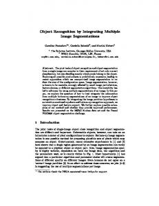
Currently, we investigate two possible applications: Exploration of parameter space and segmenter combination. Exploring Parameter Space without Ground Truth: Segmentation algorithms mostly have some parameters and their optimal setting is not a trivial task. Figure 1 shows two images segmented using exactly the same parameter set. In case (b) a nearly perfect segmentation can be achieved while we obtain a very bad segmentation in (a). Note that in this work we use the F-measure [8] (weighted harmonic mean of precision P and recall R) to quantitatively evaluate the quality of a segmentation against corresponding human GT segmentations. In recent years automatic parameter training has become popular, mainly by probing a subspace of the parameter space by means of quantitatively comparing with a training image set with (manual) ground truth segmentation [1,9]. We propose to apply the multiple segmentation combination for implicitly exploring the parameter space without the need of ground truth segmentation. It is assumed that we know a reasonable subspace of the parameter space (i.e. a lower and upper bound for each parameter), which is sampled into a finite number N of parameter settings. Then, we run the segmentation procedure for all the N parameter settings and compute a final combined segmentation of the N segmentations. The rationale behind our approach is that this segmentation tends to be a good one within the explored parameter subspace. Segmenter Combination: Different segmentation algorithms may have different performance on the same image. There exists no universal segmentation algorithm that can successfully segment all images. It is not easy to know the optimal algorithm for one particular image. We postulate: “Instead of looking for the best segmenter which is hardly possible on a per-image basis, now we look for the best segmenter combiner”. The rationale behind this idea is that while none of the segmentation algorithms is likely to segment an image correctly, we may

(a)

(b)

Fig. 1. Segmentations produced by using the FH segmentation algorithm [3] given the same set of parameter values. (a) R = 0.1885, P = 0.5146, F = 0.2759. (b) R = 0.7852, P = 0.9523, F = 0.8607.

216

P. Wattuya, X. Jiang, and K. Rothaus

benefit from combining the strengths of multiple segmenters. For this purpose we may apply various segmentation methods (each perhaps run with multiple parameter sets) to build a segmentation ensemble. In both application scenarios we need a robust combiner. It takes an ensemble S = {Si , ..., SN } of N segmentations and computes a final segmentation result S ∗ which is superior to the initial segmentations in a statistical sense (to be specified later).

3

The Multiple Segmentation Combination Algorithm

The segmentations ensemble can be produced by using different segmentation algorithms or with the same segmentation algorithm but different parameter values. We introduce the use of random walker to the problem of multiple segmentation combination. It is based on the random walker algorithm for image segmentation [4]: Given a small number of K pixels with user-defined labels (or seeds), the algorithm labels unseeded pixels by resolving the probability that a random walker starting from each unseeded pixel will first reach each of the K seed points. A final segmentation is derived by selecting for each pixel the most probable seed destination for a random walker. The algorithm can produce a quality segmentation provided suitable seeds are placed manually. The random walker algorithm [4] is formulated on an undirected, weighted graph G = (V, E), where each image pixel pi has a corresponding node vi ∈ V . The edge set E is constructed by connecting pairs of pixels that are neighbors in a 4-connected neighborhood structure. Each edge eij has a corresponding weight wij which is a real-value measure of the similarity between the neighboring pixels vi and vj . Given such a graph and the seeds, the probability of all unseeded pixels reaching the seeds can be efficiently solved. In principle there exists a natural link of our problem at hand to the random walker based image segmentation. The input segmentations provide strong hints about where to automatically place some seeds. Given such seed regions we are then faced with the same situation as image segmentation with manually specified seeds and can thus apply the random walker algorithm [4] to achieve a quality final segmentation. To develop a random walker based segmentation ensemble combination algorithm we need three components: Generating a graph to work with (Section 3.1), extracting seed regions (Section 3.2) and computing a final combined segmentation result (Section 3.3). 3.1

Graph Generation

In our context the weight eij should indicate how probably the two pixels pi and pj belong to the same image region. Clearly, this can be guided by counting the number nij of initial segmentations, in which pi and pj share the same region label. Then, we define the weight function as a Gaussian weighting: wij = exp (−β(1 −

nij )) N

(1)


217

where β is a free parameter of the algorithm. Low edge weights indicate high probabilities that there exists region boundary evidence between two neighboring pixels and avoid a random walker crossing these boundaries. 3.2

Seed Region Generation

We describe a two-step strategy to automatically generate seed points: (i) extracting candidate seed regions from G and (ii) grouping (labeling) them to form final seed regions to be used in the combination step. Candidate Seed Region Extraction: It proceeds as follows: 1. Build a new graph G∗ by removing edges whose weight in G is lower than a threshold t0 ∈ [0, 1] and work with G∗ subsequently. 2. Determine all connected components consisting of nodes with degree 4. 3. Extend each connected component C by adding those nodes which are connected to C by a chain of edges. It may happen that a node can be added to two different connected components Ci and Cj . In this case Ci and Cj are merged. The resulting connected components build a set of initial seed regions which are further refined in the next step. Note that step 1 basically deletes those edges between two neighboring nodes (pixels) which are very unlikely to belong to the same region. Grouping Candidate Seed Regions: The number of candidate seed regions from the last step is typically higher than the true number of regions in an input image. Thus, a further reduction is performed by iteratively merging the two closest candidate seed regions until some termination criterion is satisfied. For this purpose we need a similarity measure between two candidate seed regions and a termination criterion. Recall that in the initial graph G the edge weights ekl indicate how probably two pixels pk and pl belong to the same image region. This interpretation gives us a means to estimate how probably two candidate seed regions Ci and Cj belong to the same region. For a node pk ∈ Ci we consider the probability P (pi , Cj ) that when starting from pi , a random walk will reach any node in Cj . Then, we define the similarity between Ci and Cj by: Similarity(Ci , Cj ) =

1 [ max P (pk , Cj ) + max P (pl , Ci )] pl ∈Cj 2 pk ∈Ci

(2)

Note that these similarity values can be efficiently computed by the baseline random walker algorithm [4]; the full details are not given here due to the space limitation. We iteratively select two candidate seed regions with the highest similarity value and merge them to build one single (spatially disconnected) candidate seed region. This operation is stopped if the highest similarity value is below a threshold tmerge . Obviously, tmerge determines the final number K of seed regions and the segmentation combination result. Further discussion will follow later.

218

3.3


Segmentation Ensemble Combination

Given the graph G constructed from the initial segmentations and the automatically determined K seed regions, we apply the random walker algorithm [4] to compute the combination segmentation. The computation of random walker probabilities can be performed exactly without the simulation of random walks, but by solving a sparse, symmetric, positive-definite system of equations (solving the combinatorial Dirichlet problem). Each unseeded pixel is then assigned a K-tuple vector, specifying the probability that a random walker starting from that pixel will first reach each of the K seed regions. A final segmentation is derived by assigning each pixel to the label of the largest probability. 3.4

Further Implementational Details

In the seed region extraction step the computation of all similarity values in Eq. (2) can be time-consuming since we need to run the random walker algorithm [4] Nc times (being the number of candidate seed regions). In practice, we use only a small amount of pixels per candidate seed region by sampling them along the horizontal and vertical image grid by factor 5 in each direction. Furthermore, only the first 50 largest candidate seed regions are used in the merging process and all other small candidate seed regions are deleted. This number of candidate seed regions is experimentally determined to be large enough to cover all salient natural image segments. By doing it this way, we can improve the computational performance of the algorithm without degrading the qualities of combination results.

4

Experimental Results

We have conducted a series of experiments to validate the potential of our approach in the two application scenarios. The natural images with human segmentations from the Berkley segmentation dataset [7] are used. The dataset consists of 300 images of size 481×321 or vice versa, each having multiple manual segmentations. We apply the F-measure [8] to quantitatively evaluate the segmentation quality against the ground truth. One segmentation result is compared to all manual segmentations of the image and the average F-measure is reported. We empirically set the parameters β and tmerge to 30 and 0.5, respectively, for all experiments. 4.1

Exploring Parameter Space

For this experiment series the graph-based image segmentation algorithm (FH) developed by Felzenszwalb and Huttenlocher [3] is used as the baseline segmentation algorithm. The reasons for selecting this algorithm are its competitive segmentation performance and high computational efficiency. In fact, the running time is nearly linear in the number of graph edges and very fast in practice.


F = 0.6091

F = 0.2759

F = 0.4733

F = 0.5611

F = 0.8188

F = 0.5444

F = 0.5896

F = 0.8607

F = 0.6805

F = 0.3392

F = 0.4685

F = 0.6620

F = 0.8026

F = 0.5774

F = 0.7275

F = 0.7933

F = 0.7369

F = 0.6408

F = 0.7091

F = 0.7406

F = 0.8091

F = 0.6738

F = 0.7558

F = 0.8071

F = 0.6907

F = 0.4599

F = 0.5575

(a) Combined Result(b) Worst Input (c) Median Input

219

F = 0.6156 (d) Best Input

Fig. 2. Exploring parameter space. (a) Combined segmentation results of the proposed algorithm. (b)–(d) show three input segmentations with the worst, median and the best F-measure scores, respectively.

220


F−Measure

0.6

0.55

0.5 the average performance of combined results the average performance of each individual parameter setting 0 1 2 3 4 5 6 7 8 9 10 11 12 13 14 15 16 17 18 19 20 21 22 23 24 Parameter Setting

Fig. 3. Exploring parameter space: The average performance of combined results (F=0.5948) and of each individual parameter setting results over the 300 images in the database

The algorithm has three parameters: σ is used to smooth the input image before segmentation, k is the value for a threshold function (Larger values for k result in larger components in the result), and min area is a minimum component size enforced by post-processing. We obtain multiple segmentations of an image by varying the parameter values. This way 24 segmentations are generated by fixing min area = 1500 (about 1% of image area) and varying σ = 0.4, 0.5, 0.6, 0.7, 0.8, 0.9 and k = 150, 300, 500, 700. Figure 2 shows some examples of combined segmentations produced by our method. For comparison purpose we also show the input segmentation with the worst, median and best F-measure. In some cases (e.g. the first and last example) we can even achieve some improvement against the best input segmentation. For the second image this is not true (F=0.8188 compared to the best input segmentation with F=0.8607). In this case the median input segmentation has a low F=0.5896, indicating an ensemble with a majority of relatively bad segmentations. Generally, we can observe a substantial improvement of our combination compared to the median input segmentation. These results demonstrate that we can obtain an “average” segmentation which is superior to the - possibly vast majority of the input ensemble. Indeed, this behavior can be validated on the entire database of 300 images. Figure 3 shows the average performance of all 300 images for each parameter setting in comparison with the average performance of our approach. Given the fact that we do not know the optimal parameter setting for a particular image in advance (see Figure 1), the comparative performance of our approach is remarkable and reveals its potential in dealing with the difficult problem of parameter selection without ground truth. 4.2

Combination of Segmenters

In this experiment series we use the FH algorithm and multiscale Normalized Cuts (NCuts) algorithm [2] to generate multiple segmentations. While FH tends


221

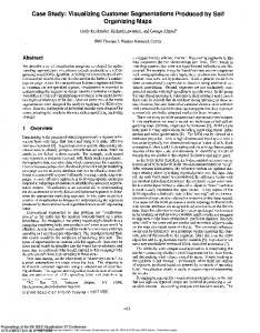
to produce small over-segmented regions, NCuts algorithm aims to produce a global segmentation with large segments that have a chance to be objects. We generate 6 different segmentations from each algorithm by varying the parameter values. For FH algorithm, we fix min area = 1500 and k = 500, and vary σ = 0.4, 0.5, 0.6, 0.7, 0.8, 0.9, and for NCuts algorithm, the parameter configuration is the number of segment k = 4, 6, 8, 10, 12, 14 and a fixed image scale 80%. One result is shown in Figure 4. For this particular image NCuts achieves higher scores, in some sense simulating a situation where the different segmentation algorithms are complementary. Again, we generally do not know which algorithm works best for a particular image. Our approach helps us to figure out the best out of all input segmentations, as exemplified in Figure 4 (bottom) with a combination result better than the entire segmentation ensemble. The average performance for all 300 images with regard to each of the 12 individual configurations (segmenter and parameter setting) is shown in Figure 5 (The first 6 configurations correspond to FH algorithm while the others are from NCuts). We also draw the red line for the performance of our combination approach of all 300 images. Without knowing the best segmenter (and the related

FH (0.5544)

FH (0.4976)

FH (0.5334)

FH (0.3429)

FH (0.4832)

FH (0.5992)

NCuts (0.5533)

NCuts (0.5839)

NCuts (0.6624)

NCuts (0.6789)

NCuts (0.6790)

NCuts (0.6799)

F = 0.7303 Fig. 4. Example of segmentation ensemble from two segmentation algorithms (top, values in parenthesis are F-measure). The combination result (bottom).

222

P. Wattuya, X. Jiang, and K. Rothaus 0.6

0.55

F−Measure

0.5

0.45

0.4

0.35 the average performance of combined results the average performance of each individual parameter setting 0.3 0

1

2

3

4

5 6 7 8 Parameter Setting

9

10

11

12

Fig. 5. Combination of segmenters: The average F-measure of combined results is 0.5902; the average F-measure of the best segmenter (6) is 0.5602

optimal parameter values in our tests) for a particular image our approach is useful for overcoming the segmentation imperfections by using multiple segmenters (and parameter values). 4.3

Discussions

The proposed algorithm was implemented in MatLab on an Intel Core 2 CPU. For a 481 × 321 image approximately 2.5 seconds are required for the seed region extraction step (Section 3.2) and less than 2 seconds for the random walker algorithm for the final combination step (Section 3.3). Regardless of the particular segmentation algorithm(s) and the thresholds of our combination algorithm, the size of segmentation ensemble can play an important role for the combined result accuracy. Increasing the size of segmentation ensemble may result in increasing both true boundary segments and false boundary segments. False boundary segments, that are shared among most of input segmentations, will most likely propagate into the final combined result. An example of this problem can be observed in Figure 4. The over-segmentation of the calf in most of the input segmentations leads to its over-segmentation in the combined result. On the other hand, decreasing the size of segmentation ensemble may result in decreasing chances of having true boundary segments. However, this problem is basically inherent to all combination algorithms that are based on co-association values voting by a segmentation ensemble.

5

Conclusion

The difficult image segmentation problem has various facets of fundamental complexity. In general it is hardly possible to know the best segmenter and for a particular segmenter the optimal parameter values. The segmenter/parameter selection problem has not received the due attention in the last. For the parameter selection problem, for instance, the researchers typically claim to have


223

experimentally fixed the parameter values or train in advance based on manual ground truth. As we have discussed before, these approaches are not optimal and it lacks an adaptive framework for dealing with the problem in a more general context. We have taken some steps towards a framework of multiple image segmentation combination based on the random walker idea. In contrast to the few works so far we consider the most general class of segmentation combination, i.e. each input segmentation can have an arbitrary number of regions. We could demonstrate the usefulness of our approach in two application scenarios: Exploring parameter space and Combination of segmenters. The results show the effectiveness of our combination method in both situations. While the preliminary results are very promising, several issues remain. The seed region generation part of our algorithm, particularly the termination criterion, needs to be further refined. Other future work includes an extension of the random walker based combination approach to other problem domains.

References 1. Cingue, L., Cucciara, R., Levialdi, S., Martinez, S., Pignalberi, G.: Optimal range segmentation parameters through genetic algorithms. In: Proc. of 15th Int. Conf. on Pattern Recognition, vol. 1, pp. 474–477 (2000) 2. Cour, T., Benezit, F., Shi, J.: Spectral segmentation with multiscale graph decomposition. In: Proc. of CVPR, pp. 1124–1131 (2005) 3. Felzenszwalb, P., Huttenlocher, D.: Efficient graph-based image segmentation. Int. Journal of Computer Vision, 167–181 (2004) 4. Grady, L.: Random walks for image segmentation. IEEE Trans. Patt. Anal. Mach. Intell 28, 1768–1783 (2006) 5. Jiang, T., Zhou, Z.-H.: SOM ensemble-based image segmentation. Neural Processing Letters 20, 171–178 (2004) 6. Keuchel, J., K¨ uttel, D.: Efficient combination of probabilistic sampling approximations for robust image segmentation. In: Franke, K., M¨ uller, K.-R., Nickolay, B., Sch¨ afer, R. (eds.) DAGM 2006. LNCS, vol. 4174, pp. 41–50. Springer, Heidelberg (2006) 7. Martin, D., Fowlkes, C., Tal, D., Malik, J.: A database of human segmented natural images and its application to evaluating segmentation algorithms and measuring ecological statistics. In: Proc. 8th Int. Conf. Computer Vision, vol. 2, pp. 416–423 (2001) 8. Martin, D., Fowlkes, C., Malik, J.: Learning to detect natural image boundaries using local brightness, color, and texture cues. IEEE Trans. Patt. Anal. Mach. Intell. 26(5), 530–539 (2004) 9. Min, J., Powell, M., Bowyer, K.W.: Automated performance evaluation of range image segmentation algorithms. IEEE Trans. on SMC – Part B 34(1), 263–271 (2004) 10. Rohlfing, T., Russakoff, D.B., Maurer Jr., C.R.: Performance-based classifier combination in atlas-based image segmentation using expectation-maximization parameter estimation. IEEE Trans. Medical Imaging 23, 983–994 (2004) 11. Rohlfing, T., Maurer Jr., C.R.: Shape-based averaging for combination of multiple segmentations. In: Duncan, J.S., Gerig, G. (eds.) MICCAI 2005. LNCS, vol. 3750, pp. 838–845. Springer, Heidelberg (2005)