Combinatorial Interaction Regression Testing: A Study of Test Case ...

Combinatorial Interaction Regression Testing: A Study of Test Case Generation and Prioritization Xiao Qu, Myra B. Cohen, Katherine M. Woolf Department of Computer Science and Engineering University of Nebraska-Lincoln {xqu,myra,kwoolf}@cse.unl.edu

Abstract Regression testing is an expensive part of the software maintenance process. Effective regression testing techniques select and order (or prioritize) test cases between successive releases of a program. However, selection and prioritization are dependent on the quality of the initial test suite. An effective and cost efficient test generation technique is combinatorial interaction testing, CIT, which systematically samples all t-way combinations of input parameters. Research on CIT, to date, has focused on single version software systems. There has been little work that empirically assesses the use of CIT test generation as the basis for selection or prioritization. In this paper we examine the effectiveness of CIT across multiple versions of two software subjects. Our results show that CIT performs well in finding seeded faults when compared with an exhaustive test set. We examine several CIT prioritization techniques and compare them with a re-generation/prioritization technique. We find that prioritized and re-generated/prioritized CIT test suites may find faults earlier than unordered CIT test suites, although the re-generated/prioritized test suites sometimes exhibit decreased fault detection.

1. Introduction Regression testing is an expensive part of the software process. As systems evolve, before new versions are released, software must be re-tested to ensure quality. One concern in regression testing is the effectiveness of test suites in finding new faults in successive program versions. A second issue is the efficiency of running the test suites given limited resources and time. Small test suites that retain high fault detection ability are desirable. A focus of regression testing research has been the reduction of test suite size between versions. This can be accomplished through test suite selection [15]. A further improvement, once tests

are selected, is to order or prioritize [16] test cases to increase the likelihood of faults being discovered early in the test process. Detecting faults early, means that work to repair faults can begin sooner, and if resources are exhausted before all tests complete, the consequences are less severe. Although much of regression testing research has focused on test suite selection and prioritization, the original test suite generated and used during the lifetime of evolving software is also important. The quality of this test suite sets the upper bound for the quality of selected tests, and impacts the ability to order test suites effectively in all successive versions. One specification based test generation technique is to use the category partition method and the Test Specification Language or TSL [14] to define program parameters and environments and partition the resulting categories into choices. The choices are combined to generate test cases. Constraints are added to categories and choices to reduce the test space since combining all choices of these categories results in a combinatorial explosion. A related specification based technique for generating test suites is combinatorial interaction testing [3, 5, 6, 12, 19] or CIT, although less is known about its use in regression testing. In CIT the program is divided into partitions as in TSL. To reduce the final number of test cases, parameters are tested together so that all t-way combinations appear at least once. This technique has been shown to produce small test suites, with high code coverage, that exhibit good fault detection ability [5, 7, 19]. Although CIT has shown to be an effective test generation technique, it has mostly been examined in the context of single version software systems. There has been little research examining the effectiveness of CIT in regression testing, applied across evolving versions of a software program. Furthermore, there is no work that applies prioritization techniques to such an environment. In [4] Bryce and Colbourn present an algorithm to prioritize CIT test suites. They do not, however, experiment on real software subjects, nor do they address the key element of weighting the vari-

ous elements that drive prioritization. Additionally, it is our observation that their prioritization technique is a combined generation and prioritization technique, rather than pure prioritization, since it does not re-order tests, but re-generates them each time. We call this technique re-gen/prio. This is similar to the work of Avritzer et al. [2] who also present an ordered test generation technique. This leaves us with several questions. We would like to understand if CIT is effective when used in regression testing for multiple versions of a program. We would also like to understand if prioritization improves early fault detection in CIT test suites, and finally, we would like to understand how to prioritize CIT test suites. In this paper we address each of these issues. We have conducted an empirical study on two software subjects, each with multiple successive versions. We first examine the effectiveness of CIT test suites compared with an exhaustive strategy. We then apply both prioritization and regen/prio and compare their effectiveness on CIT test suites. We examine several different ways to control the prioritization. We use methods that leverage code coverage from prior releases, as well as one that is specification based. Our results show that the CIT test suites may be an effective way to reduce the test space and that prioritization improves the ability to detect faults early in certain subjects. The rest of this paper is organized as follows. Section 2 presents related work on regression testing and combinatorial interaction testing, Section 3 discusses prior work on prioritization algorithms for CIT and presents methods for weighting the prioritization. Section 4 introduces our empirical study. Section 5 presents our results and Section 6 concludes and presents future work.

2. Background In this section we provide some background on regression testing and combinatorial interaction testing.

2.1. Test Case Selection and Prioritization The test case selection problem can be stated as follows. Given an initial version of a program P and a set of test cases, T , select a subset of tests from T , T 0 to test a new version of program P , P 0 [16]. The simplest method is to re-test all. However, this suffers from the problem of accumulating too many tests over time. Other techniques include code coverage , dataflow, minimization, safe and ad-hoc/random [10]. In this paper we do not address the test case selection problem. Instead we generate CIT test suites that are already small in size and use the re-test all approach. Prioritization techniques [9, 13, 16, 17] complement the selection technique. In prioritization test cases are ordered to improve the likelihood that faults will be detected

early in the testing process. Techniques for prioritization include statement coverage, function coverage and fault finding exposure, among others [9, 13, 16, 17].

2.2. Test Case Specification Language The Test Specification Language [14] is a specification based method to define the combinations of program parameters that should be tested together. TSL partitions the system inputs into parameters and environments which make up the categories. For each of these, a set of choices is defined based on equivalence classes of the input domain. Two methods are used to reduce the large combinatorial space caused by the combination of all input parameters. The first method sets specific choices as single or error, meaning that these options are tested alone. The second is to add properties to particular choices and define constraints that relate other choices to these properties. This has the effect of significantly reducing the final set of combinations. In TSL all possible combinations, are generated given the set of specified constraints.

2.3. Combinatorial Interaction Testing An alternate way to subset the test cases is combinatorial interaction testing (CIT) [5]. It is still possible to use TSL to define categories and choices, but CIT differs from TSL in that it provides a systematic sampling of the input space. Constraints are only used in CIT when they are enforced by the underlying system. In CIT the categories are called factors and each factor has a set of values (choices in TSL). A CIT test suite samples the input space so that it includes all t-way combinations of values between factors, where t is called the strength of testing. For instance when t=2, we call this pair-wise testing. CIT samples are defined by mathematical objects called covering arrays. A covering array, CA(N ; t, k, v), is an N ×k array on v symbols with the property that every N ×t sub-array contains all ordered subsets from v symbols of size t at least once [6]. Quite often in software testing the number of values for each factor is not the same. Therefore, we use the following expanded definition (often called a mixed level covering array) that uses a vector of vs for the factors. A mixed level covering array, CA(N ; t, k, (v1 v2 ...vk )), Pk is an N × k array on v symbols, where v = i=1 vi , where each column i (1 ≤ i ≤ k) contains only elements from a set Si of size vi and the rows of each N × t sub-array cover all t-tuples of values from the t columns at least once. We use a shorthand notation to describe these arrays with superscripts to indicate the number of factors with a particular number of values. For example, a covering array with 5 factors, 3 of which are binary and 2 of which have four values

can be written as follows: CA(N ; 2, 32 24 ). (we remove the k since it is implicit). Covering arrays have been shown to be effective test suites in a variety of studies [3, 5, 12, 19].

CA(N;2,3221) values for each factor F0=0 ,1,2 F1=3,4,5 F2=6,7

3. Prioritization Techniques

Count of Values Value 0

Before we can assess the effectiveness of CIT test suites in regression testing, we must first determine how to prioritize. We present background on a prioritization algorithm next and follow this with a discussion of techniques that we have developed to make this algorithm work in practice.

3.1. Re-generation In [4] the authors describe an algorithm for re-generating prioritized test suites. The test suites generated are a special kind of a covering array called a biased covering array. They begin by defining a set of interaction weights for each value of each factor. For each factor the weight of combining it with each other factor is computed as a total interaction benefit. The factors are sorted in decreasing order of interaction benefit and then filled as follows. First, the individual interaction weights for each of the factor’s values is computed. (see [4] for more details). This selects the value of the factor that has the greatest value interaction benefit. After all factors have been fixed, a single test has been added, and the benefits for factors are recomputed and the process starts again. The algorithm is complete when all pairs have been covered. The pseudo-code for this algorithm is presented in Algorithm 1.

3.2. Assigning Weights In the re-generation algorithm [4] methods for setting weights are not presented, yet the weighting method may play an important role in how well the algorithm performs. For the purpose of our study we try three code coverage based weighting methods and one specification based method. We describe each in turn. 3.2.1

Code Coverage Based Weightings

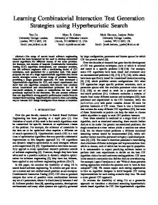
We begin by greedily ordering the current CIT test suite using cumulative code coverage. The first test case is the one that provides the highest branch coverage. We add tests until we have reached the total branch coverage found in the full test suite. In the first weighting scheme we count the number of occurrences of each value in the newly ordered sample, and divide it by the number of test cases in counti . Figure 1 shows an example the sample, i.e. wi = count tests with three factors, F0 , F1 and F2 . There are three test cases from the prior version that contribute to the total cumulative branch coverage. The array on the bottom shows the count

Test Cases 0 4 6 0 5 7 0 3 7

F0 F1 F2

3 1 1

Value 1

Value 2

0 1 2

0 1

Figure 1. Example of Setting Weights

of the values. For instance, value 0 of F0 (0) occurs 3 times in the test suite, while value 1, of F2 (7) occurs twice. The weights for F0 will be 1, 0, 0, for F1 will be 0.33, 0.33, 0.33 and for F2 will be 0.33 and 0.66. The second weighting scheme performs the same initial weighting and then multiplies this by a factor weight. For w i where wmaxi is each factor, Fi , the weight equals wmax max the maximum count of a value in Fi , and wmax equals the maximum of all wmaxi s. The weights of the factors in Figure 1 are 1, 0.33 and 0.66. The final weights for the values in Figure 1 are 1, 0, 0 for F0 , 0.332 , 0.332 , 0.332 for F1 and, 0.66 × 0.33, 0.662 for F2 . This weighting is meant to normalize factors that have a small number of values which dominate the counts. Our third weighting scheme tries to utilize more of the information in the original test suite, since there may be more than one test case with equal cumulative coverage at each stage. For this weighting we use a parallel approach. We begin with an expansion, followed by a collapse stage. We start with the first four test cases that provide the highest cumulative coverage. (In our study subjects we found this provides over 90% of the total branch coverage). We then expand as follows. For each of the four tests we find all other test cases in the CIT test suite that will provide equivalent coverage. For instance if the first test case covers 45% of the branch coverage, we find all other test cases that also provide this coverage. We then examine the next test case. If this adds 15% more coverage we find all other test cases with the same additional branch coverage, etc. We select tests without replacement (each can belong to a single group). For each of the four groups we calculate weights for each value, by counting its occurrence as was done in the first weighting scheme, and dividing by the number of test cases in that group. For the collapse stage, we first set an importance, I to each of the four groups. The first group contains all of the tests with the highest individual code coverage. This is assigned I = 0.6. The next group is assigned I = 0.2, while the last two groups are set to I = 0.1. The weight of each value is multiplied by its importance I, and the four weights are summed to obtain the individual weight for that value. Figure 2 illustrates this process.

Collapse Final Weights

Expand

0 1 2 1 2 3 1

Test Cases 4 4 5 3 … 4 4 4

6 7 7 6 6 6 6

w i1 = 0.6(

count ) testcases

w i2 = 0.2(

count ) testcases

w i3 = 0.1(

count ) testcases

w i4 = 0.1(

count ) testcases

! ! !

Add test cases to each array above with Same cumulative ! coverage

4

TotalWeight(Valuei )" w ij j=1

! Figure 2. Third Weighting Scheme

RemainingP airs = AllP airs while RemainingP airs 6= ∅ do Compute Interaction Weights for Factors OrderFactors for i = 1 to numF actors do SelectHighestWeightUnfixedFactor for j = 1 to numV alues do Compute Interaction Weights for Factor Values SelectValue with highest weight Add Test Case

Algorithm 1: Re-gen/Prio Algorithm [4]

3.2.2

Specification Based Weightings

There may be instances where we do not have prior code coverage. In these scenarios we want to weight our test cases using the specifications. Since we define our test partitions using TSL we use this for weighting. Our initial heuristic works as follows. For each category we examine the possible choices. In the case of binary choices, where one choice turns a feature on and one turns a feature off we set the ON option to a weight of 0.9 and the OFF option to 0.1. Our intuition is that the ON option will cause more code to be executed. In cases where we have multiple choices, we use a greater number of features or higher complexity of the choice as a proxy for higher code coverage. For instance in the subject make, we have a partition that includes choices to test no files, one file, two files, or five files. We set a weight of 0.1 for the choice of no files, a weight of 0.2 for the choice of one file, ..., and a weight of 0.4 for the choice of five files. Similarly in the subject flex one parameter controls table compression. We put higher weights on those options that perform more complex compression tasks ( For instance, we set a weight of 0.1 for -C, 0.2 for -Cr,..., and 0.5 for -Craem.) In initial experimentation we found that this gives us the most consistent results in relation to the prioritized exhaustive set of test cases used in our study. Different heuristics may impact the quality of this method, but we leave this for future work.

3.3. Pure Prioritization We use two different methods to prioritize the CIT test suites. The first method uses branch coverage from the prior version. This is a standard prioritization technique [9]. For program P we use cumulative branch coverage in the CIT test suite, ordering until we reach 100% coverage of the CIT test suite. The remaining tests are left in their original order. The second method is to use the interaction weighting method, but rather than re-generate we simply use it to order the given tests based on their weights. We use the weighting schemes described above and for each test case calculate its interaction weight. We then sort the tests in decreasing order of interaction weight.

4. Empirical Study In this section we present an empirical study to investigate the applicability of using CIT in regression testing. We have designed experiments to answer the following three research questions: RQ1: Is CIT an effective test generation technique for regression testing compared with an exhaustive test suite? RQ2: Do prioritized and/or re-gen/prio CIT test suites exhibit earlier fault detection when compared with nonprioritized CIT test suites? RQ3: Can we prioritize and/or re-gen/prio CIT test suites without code-coverage information? The rest of this section describes our objects of analysis, our metrics and our methodology.

4.1. Objects of Analysis We have used two C subjects, each with multiple successive versions. The subjects were obtained from the software infrastructure repository (SIR) [8]. The first subject, flex is a lexical analyzer. The other subject, make is used to compile programs. Table 1 shows the uncommented lines of code for each version of the program, the number of functions and the number of changed or added functions between versions. We used the SLOCCount tool [18] to count the uncommented lines of code and the adiff utility from the SIR repository [8] to determine changed methods. These were manually verified for the purposes of seeding new faults. Each subject came with a TSL test suite and between 5-20 hand seeded faults. Hand seeding allows us to turn faults on and off during experimentation. The number of seeded faults in each subject is also shown in Table 1. To increase our ability to reason about the final results, we seeded an additional 30 faults into each subject, using a C mutation test case generator written by Andrews et al. [1]. Their research indicates that mutation faults produce similar

results in empirical studies as hand seeded faults. We generated all mutants for each program. To simulate a regression environment, we identified the changed and added functions between consecutive versions of the programs and selected only mutants contained in those areas of the code We then randomly selected the first 30 that successfully compiled. To answer RQ1 we created new reduced TSL files that were unconstrained. We retained the most widely used features in each subject (based on the man pages) and ran some experiments using the original set of hand-seeded faults. Our objective was to obtain exhaustive suites that retain close to the original fault detection ability. We note that in a real test environment an unconstrained TSL would most likely be prohibitive in size and would not be used. Table 2 shows some comparative data between the TSL suites. It shows the number of test cases, the number of faults found and the percentage of branch and statement coverage. The faults detected consist of the original hand seeded faults and the total number of faults. Our tuning was performed using the original hand seeded faults only; the mutation faults were seeded after we developed the exhaustive test suite. The new test suites have the same fault detection for the original seeded faults, but slightly lower fault detection for the new mutation faults. The code coverage of the new test suite is slightly lower as well. We attribute this partly to the removal of the error conditions that make up a portion of the TSL test suite. Subject flex V0 V1 V2 V3 V4 V5 make V0 V1 V2 V3 V4

uLoC

Function Count

# Changed Functions

Seeded Faults

7,972 8,426 9,932 9,965 10,055 10,060

138 147 162 162 162 162

NA 40 104 24 16 13

NA 49 50 47 46 39

12,612 13,484 14,014 14,596 17,155

188 190 206 239 270

NA 80 88 158 145

NA 38 36 35 35

Table 1. Test Subjects Studied

4.2. Independent Variables Our independent variables are the various test suites that we have generated and/or prioritized. The first data set is the exhaustive set of data which we label full. This contains all possible combinations of the parameters from the TSL specification in the order it was generated.

Subject flex V1 Orig. TSL Full make V1 Orig. TSL Full

# Test Cases

Detected Tot. Faults

Detected Orig. Faults

Branch Cov

Stmt Cov

525 4,608

38 33

16 16

73.1% 60.5%

72.9% 61.8%

796 4,320

11 10

4 4

41.4% 38.3%

40.0% 38.5%

Table 2. Full Test Suite vs. Original TSL

CIT Specification flex CA(N ; t, 24 31 161 61 ) make CA(N ; t, 31 22 51 32 21 41 )

Size t=2

Size t=3

Size t=4

Size t=5

96

288

NA

NA

20

60

180

540

Table 3. Size of CIT Test Suites

We generated 50 t-way covering arrays using simulated annealing [6] with t set to 2 and 3 for flex, and 2, 3 and 4, and 5 for make. The sizes of these arrays are shown in table 3. We label these as t = 2, etc. in our experiments.We also generated 50 random arrays of the same size, labeled rdt where t corresponds to the strength of a CIT test suite. We include a prioritization “oracle” based on the full branch coverage of the full test suites. Since this is a standard prioritization technique and the exhaustive test set has the maximum possible information given our TSL specification, we use this to see how well other techniques perform. We call this p-full. For the CIT techniques we include a code coverage prioritization baseline using branch coverage prioritization on a strength 2 and strength 3 covering array. We call these bp-t=2 and bp-t=3. For the experimental techniques, we use an individual CIT test suite for program P and prioritize it based on branch coverage as above. We then use the weighting schemes and algorithms discussed in section 3 to either regen/prio or prioritize for version P +1. We only show the last weighting scheme in our results, since it gave us the most consistent results. We call these p-t=n, r-t=n where p stands for prioritized and r stands for re-gen/prio. The value of n is the strength of the CIT test suite that was used. Finally, for the TSL based weighting, we developed a single weighting scheme (as described in section 3) and applied this to each of the CIT test suites for the prioritization or used it to re-generate a new CIT suite. The re-gen/prio TSL CIT suite has only one prioritized test suite across versions, since all of the TSL CIT suites, use the same set of tests across all versions; i.e. we did not change the TSL specifications during testing. We call these test suites, r-tsl and p-tsl for re-gen/prio and prioritization respectively.

1 T F1 + T F2 + ... + T Fm + m×n 2n In this formula there are n test cases and m faults. T Fi stands for the number of the test case (when testing in prioritization order) in which Fault i was found. For instance in Figure 3, T F2 , T F4 and T F7 all have a value of 1, while T F5 and T F6 are 2. One drawback of the above formula is that it uses the entire area of the graph. It assumes that m and n do not change since it usually only examines prioritization rather than regen/prio where both test suite size and fault detection may differ. In our experiments, it is possible that two variations occur. First, we may not find all of the faults using a particular test suite and second, we may not run the same number of tests. To handle the second problem we fix the number of test cases to be the size of a t=2 covering array and only examine the area up until that point in time (x-axis). This is shown in the right part of Figure 3. We still need to adjust for the missing faults. In [17] Walcott et al. present a similar problem. Their solution is to assign a penalty to the missed faults which allows their APFD to become negative. We want our metric to continue to reflect the actual area under the curve, which cannot be negative, so we have re-derived the formula using the following geometry (we leave out the full derivation). The original APFD can be equated with the area of the curve as follows: (see left side of Figure 3). The full area is 1.0. To find the area outside of the curve we divide it into horizontal rectangles. This is subtracted from the full area (and is represented by the middle part of the equation). However, the triangles still need to be added back in to represent the full area under the curve. This is the last part of 1 . There are n triangles (one for each test the equation, 2n case) shaded in Figure 3. (we can have triangles with zero area, as is seen in this Figure) A new formula which we call the Normalized APFD is the result (shown on the right side of Figure 3). We use this to measure the effectiveness of prioritization since it includes information on both fault finding and time of detection.

1.0

8 7

0.625

Percent of Faults Detected

In [9, 16] a metric that is commonly used for prioritization is the Average Percentage of Faults Detected or APFD. This metric measures the area under the curve when the percent of faults found is plotted on the y-axis and the percent of the test cases run on the x-axis. Figure 3 (left) shows this type of graph which represents tests in Table 4. In this fault matrix, there are 5 tests and 8 faults. The ordering of the test cases is T3 , T5 , T2 , T4 , T1 . The first test (or 20% of the test cases) finds 3 faults. After 3 test cases or 40% of the test cases, 5 faults have been found or 62.5 %. To calculate the APFD the following formula is given in [9]:

1.0

Percent of Faults Detected

4.3. Dependent Variables

5

0.5

0.0

0.2

0.4

0.6

0.8

1.0

Tests not run

5

0.0

Percent of Test Suite Run

0.33

0.66

1.0

Percent of Test Suite Run

APFD (8 faults, 5 test cases)

NAPFD (After 3 test cases)

Figure 3. Example of APFD and NAPFD

AP F D = 1 −

N AP F D = p −

T F1 + T F2 + ... + T Fm p + m×n 2n

where p = the number of faults detected by the prioritized test suite divided by the number of faults detected in the full test suite (y-axis). If a fault, i, is never detected we set T Fi = 0. The NAPFD in Figure 3 is 0.44. T1 F1 F2 F3 F4 F5 F6 F7 F8

T2

T3

x

x

T4 x

T5

x x

x x

x x x

x

Table 4. Test Order: T3 , T5 , T2 , T4 , T1

4.4. Study Methodology For each set of experiments we run all tests on each subject without any faults as an oracle and then turn on each fault individually. We collect branch coverage on the fault free version using the Aristotle coverage tool [11]. We only include faults in our results that occur between 0 and 50 % of the time in the exhaustive test suite. Our rationale is that faults occurring more than 50 percent of the time will be very easy to find and would be eliminated during unit testing. (we note that Table 2, which compares the original TSL suite, and the reduced exhaustive TSL suite, includes all faults regardless of how often they are found). For data using CIT test suites or random test suites, we take the average of 50 arrays to prevent biases due to chance. For all of our re-gen/prio and prioritization experiments we use program P to prioritize program P +1. For each of our subjects

1.0

FLEX−V2

●

● ● ● ● ● ● ● ● ● ● ● ● ● ● ● ● ● ● ● ● ● ● ● ● ● ● ● ● ● ● ● ● ● ● ● ● ● ● ● ● ● ● ● ● ● ● ● ● ● ● ● ● ● ● ● ● ● ● ● ● ● ● ● ● ● ● ● ● ● ● ● ● ● ● ● ● ● ● ● ● ● ● ● ● ● ● ● ● ● ● ●●●●●●●●●●●●●●●●●●●●●●●●●●●●●●●●●●●●●●

●●●●●●

●

●●●●●●

●

●●●● ●●●

0.8

●●

●●●●●●

●●

●●

●

0.6

●

●● ●

t=2 t=3 p−full bp−t=2 p−t=2 p−tsl r−t=2 r−tsl

● ● ● ●

●

●

●

0

20

40

5. Results

60

80

100

Number of test cases

Figure 4. Cum. Fault Coverage: flex V2

●

●

●

●

●

●

0.6

●

●

●

●

●

●

●

●

●

●

●

●

●

●

●

●

●

●

● ●

● ●

● ●

● ●

●

t=2 t=3 p−full bp−t=2 p−t=2 p−tsl r−t=2 r−tsl

●

0.4

Percentage of faults detected

0.8

1.0

MAKE−V1

●

●

●

0.2

●

● ●

●

●

0.0

To answer RQ1 related to whether CIT is an effective test generation technique, we examine the fault detection ability of different strength CIT test suites. Figure 6 shows the results of testing across all versions of both software subjects. For flex (the top part of the figure) we show the full test suite, followed by a t=2 CIT test suite, followed by a random suite of the same size. We then show both a t=3 and corresponding random size suite next. Both the random and CIT test suites for t=2 miss some faults in the first 3 versions, but all of the t=3 and corresponding random suites detect all faults. The behavior of make is slightly different. In this subject we find in V1 the t=2 arrays miss faults more regularly. We see the same result with t=3. However, as the strength of t is increased our fault detection improves. In this subject we see that the t=2 array has better fault detection than a random test suite of the same size. We examined the fault that was missed by some of the t=5 suites. This is a fault that occurred rarely (less than 2% of the time) in the exhaustive suite and is likely caused by a high level interaction. Next we explore RQ2, which asks if prioritized or regen/prio CIT test suites exhibit earlier fault detection. If we examine Figure 4 we see the cumulative fault coverage of flex for various techniques. We show the full test suite prioritized as a benchmark, since we expect this is created with the most information. We see that the prioritized t=2

●●●●

●●●●●●

● ●●●● ●●● ●

●

0.4

Percentage of faults detected

Empirical experiments suffer from threats to validity. We have made attempts to reduce these, however, we outline the major threats here. With respect to external validity (or the threat of generalizing to other subjects) we acknowledge that we have only examined two software subjects, both of which were written in the C language. We have tried to select two different subjects, of different sizes and for each have used multiple versions of the program. But results obtained from other subjects may not match these. With respect to internal validity (or the threat that our experiments themselves suffer from mistakes) we have tried to manually cross-validate our analysis programs on small examples and have manually validated random selections from the real results. We have made every effort to ensure that these are correct. As far as construct validity, (or the threat that we may not have fairly conducted these studies) we acknowledge that there may be other metrics which are more pertinent to this study. We also note that we may have developed different unconstrained TSL definitions.

0.2

4.5. Threats to Validity

test suite, based only on block coverage bp-t=2, exhibits the next best coverage. (Results for bp-t=3 provide similar results but are not shown.) One interesting note is that the covering arrays for t=3 exhibits poor growth with a very long flat tail, although when it is run to completion it consistently covers more faults than t=2. In make (Figure 5) we see similar results, although the un-prioritized t=2 array seems to do slightly better than the prioritized array using interaction weights p-t=2. This may be due to the lack of the overall quality of code coverage or may be due to the existence of higher order interaction faults.

0.0

we have a base version, V0, with no faults. We use this only to generate the prioritization for V1.

0

5

10

15

20

25

Number of test cases

Figure 5. Cum. Fault Coverage: make V1 We examine the data next using the NAPFD (Figures 7 and 8). In flex, in all but the last version we see that the first three data points, the un-prioritized full test suite, a t=2 test suite and a t=3 test suite, perform worse than both the prioritized and re-gen/prior test suites. The branch coverage based prioritization (p-full, bp-t=2, bp-t=3) seems to perform the best overall. The re-gen/prio schemes using interaction weights in general seem to find faults earlier,

Figure 6. Fault Detection: CIT vs. Random and Full however, they sometimes have reduced fault detection ability (see Figure 4) which reduces the NAPFD. For instance in V2 and V3, re-gen/prio test suites differ by three in the number of faults they detect (data not shown) whereas the prioritized test suites differ by one. In V1, fault detection of the t=2 arrays differs by one while in the re-gen/prio arrays there is a difference of two. In V3, where the re-gen/prio arrays miss as many as 3 faults in some runs, they perform even worse than random arrays of the same size. In make our results varied slightly again. Although the code coverage based prioritization for the CIT test suites seem to work best, there appears to be less difference in

the NAPFDs for the prioritized and un-prioritized covering arrays than there was in flex. Our last research question, RQ3, asks whether or not a specification based prioritization is effective. For this question we examine the TSL based re-gen/prio and prioritization in the previous figures. We see in Figure 4 that the re-gen/prio TSL finds faults earlier in flex than the prioritized TSL and both perform better than the un-prioritized CIT suites. In make (Figure 5) the re-gen/prio TSL has better fault detection than the prioritized TSL. Even the the unprioritized CIT test suites find faults earlier than the priori-

80

! ! !

!

! ! ! !

!

80

! !

FLEX!V3 100

100

FLEX!V2

80

100

FLEX!V1

!

!

! ! !

! ! ! !

!

full t=2 t=3 r!tsl r!t=2 p!full bp!t=2 bp!t=3 p!t=2 p!tsl

20

40

60

!


20


60 40

100

!

60

! !

!

80

! ! !

!

FLEX!V5

40

NAPFD

80

100

FLEX!V4

20

60 40 full t=2 t=3 r!tsl r!t=2 p!full bp!t=2 bp!t=3 p!t=2 p!tsl


20

60 20

40

NAPFD

! !

! !

Figure 7. NAPFD for flex tized TSL. Finally we examine the NAPFD. Looking at the NAPFDs for flex (Figure 7) and make (Figure 8) we see that using the re-gen/prio TSL to set weights appears to be better than using the prioritized TSL.

6. Conclusions In this paper we have examined the effectiveness of CIT on regression testing in evolving programs with multiple versions as well as studied several prioritization techniques. Our findings suggest that the use of CIT test suites in regression testing is an effective method of testing, however, the strength that is used, must be considered. In flex we found that both the prioritization and re-gen/prio techniques were effective. The re-gen/prio technique tends to miss more faults, but finds faults sooner. In make we experienced mixed results which may be due to the lower branch coverage of our test suites, or due to the small size of the CIT test suites. We also found that the specification or TSL weightings did no worse and in some cases better than the interaction based weighing scheme that used code coverage. This is promising since we may not always have code coverage information. The difficulty for this method will be finding good heuristics to weight the specifications. In both subjects we found that a standard branch based prioritization outperformed all other techniques.

In future work we are applying these techniques to additional subjects. We are looking at other prioritization techniques and at prioritizing higher strength covering arrays, and we are formalizing heuristics for the TSL based weighting. We are also examining costs of re-gen/prio vs. pure prioritization to understand the tradeoffs between these two.

7. Acknowledgments We thank L. Brown, T. Fangmeier and D. Nelson for help on the experimental infrastructure. This work was supported in part by an NSF EPSCoR FIRST award, by an NSF EPSCoR small grant, and by a UNL Layman award.

References [1] J. H. Andrews, L. C. Briand, Y. Labiche, and A. S. Namin. Using mutation analysis for assessing and comparing testing coverage criteria. IEEE Transactions on Software Engineering, 32(8):608–624, 2006. [2] A. Avritzer and E. R. Weyuker. The automatic generation of load test suites and the assessment of the resulting software. IEEE Transactions on Software Engineering, 21(9):705–716, 1995. [3] R. Brownlie, J. Prowse, and M. S. Phadke. Robust testing of AT&T PMX/StarMAIL using OATS. AT& T Technical Journal, 71(3):41–47, 1992.

100

MAKE!V2

100

MAKE!V1

!

80

80

!

!

! !

!

!

p!t=2

p!tsl

p!t=2

p!tsl

! ! !

80

80

! !

! !

!

60

! !

!

bp!t=3

bp!t=2

p!full

r!t=2

r!tsl

t=4

t=3

t=2

full 20

p!tsl

p!t=2

bp!t=3

bp!t=2

p!full

r!t=2

r!tsl

t=4

t=3

t=2

full

40

60

NAPFD

!

40

NAPFD

bp!t=3 !

!

! ! !

20

bp!t=2

p!full

r!t=2

100

MAKE!V4

100

MAKE!V3

r!tsl

t=4

t=3

t=2

full 20

p!tsl

p!t=2

bp!t=3

bp!t=2

p!full

r!t=2

r!tsl

t=4

t=3

t=2

20

full

40

!

60

NAPFD

60

!

40

NAPFD

! !

Figure 8. NAPFD for make [4] R. Bryce and C. Colbourn. Prioritized interaction testing for pair-wise coverage with seeding and constraints. Journal of Information and Software Technology, 48(10):960–970, 2006. [5] D. M. Cohen, S. R. Dalal, M. L. Fredman, and G. C. Patton. The AETG system: an approach to testing based on combinatorial design. IEEE Transactions on Software Engineering, 23(7):437–444, 1997. [6] M. B. Cohen, C. J. Colbourn, P. B. Gibbons, and W. B. Mugridge. Constructing test suites for interaction testing. In Proceedings of the International Conference on Software Engineering (ICSE), pages 38–48, May 2003. [7] S. R. Dalal, A. Jain, N. Karunanithi, J. M. Leaton, C. M. Lott, G. C. Patton, and B. M. Horowitz. Model-based testing in practice. In Proceedings of the International Conference on Software Engineering, pages 285–294, 1999. [8] H. Do, S. G. Elbaum, and G. Rothermel. Supporting controlled experimentation with testing techniques: An infrastructure and its potential impact. Empirical Software Engineering: An International Journal, 10(4):405–435, 2005. [9] S. Elbaum, A. G. Malishevsky, and G. Rothermel. Test case prioritization: A family of empirical studies. IEEE Transactions on Software Engineering, 28(2):159–182, February 2002. [10] T. L. Graves, M. J. Harrold, J.-M. Kim, A. Porter, and G. Rothermel. An empirical study of regression test selection techniques. IEEE Transactions on Software Engineering, 10(2):184–208, Apr. 2001. [11] M. J. Harrold, L. Larsen, J. Lloyd, D. Nedved, M. Page, and G. Rothermel. Aristotle: a system for development of program analysis based tools. In ACM 33rd Annual Southeast Conference, pages 110–119, 1995.

[12] D. Kuhn and M. Reilly. An investigation of the applicability of design of experiments to software testing. In Proceedings of the NASA/IEEE Software Engineering Workshop, pages 91–95, 2002. [13] Z. Li, M. Harman, and R. M. Hierons. Search algorithms for regression test case prioritization. IEEE Transactions on Software Engineering, 33(4):225–237, April 2007. [14] T. J. Ostrand and M. J. Balcer. The category-partition method for specifying and generating functional tests. Communications of the ACM, 31:678–686, 1988. [15] G. Rothermel and M. J. Harrold. Analyzing regression test selection techniques. IEEE Transactions on Software Engineering, 22(8):529–551, Aug. 1996. [16] G. Rothermel, R. Untch, C. Chu, and M. J. Harrold. Prioritizing test cases for regression testing. IEEE Transactions on Software Engineering, 27(10):929–948, Oct. 2001. [17] K. R. Walcott, M. L. Soffa, G. M. Kapfhammer, and R. S. Roos. Time-aware test suite prioritization. In International Symposium on Software Testing and Analysis, pages 1–11, 2006. [18] D. Wheeler. SLOCCount. http://www.dwheeler. com/sloccount/, 2007. [19] C. Yilmaz, M. B. Cohen, and A. Porter. Covering arrays for efficient fault characterization in complex configuration spaces. IEEE Transactions on Software Engineering, 31(1):20–34, Jan 2006.