Combinatorial Koszul Homology, Computations and Applications - arXiv

arXiv:0803.0421v1 [math.AC] 4 Mar 2008

Combinatorial Koszul Homology, Computations and Applications Eduardo S´ aenz-de-Cabez´ on Irigaray

Dissertation submitted for the degree of Doctor of Philosophy

Supervisors: Prof. Dr. Luis Javier Hernández Paricio Prof. Dr. Werner M. Seiler

Universidad de La Rioja Departamento de Matemáticas y Computación

Logro˜ no, December 2007

This work has been partially supported by project CALCULEMUS (Contract No HPRNCT-2000-00102) and GIFT (NEST Contract No 5006) from the European Union. And by project ANGI-2005/10 from the Comunidad Autónoma de La Rioja, and grants ATUR-04/51, ATUR-05/46, ATUR-06/31 from the Universidad de La Rioja.

Acknowledgments A la memoria de mi padre, de quien aprend´ı que s´ olo cuando hacemos caso al coraz´ on por encima de la raz´ on, podemos ser felices. A mi madre, que me ense˜ no ´ que s´ olo el control de la raz´ on puede llevar a buen puerto los impulsos del coraz´ on. A ambos, de cuya uni´ on he aprendido el necesario equilibrio que hace m´ as sencillo el camino de la vida. A Elena, mi amor, es decir, mi vida. A Juan, Luc´ıa y M´ıkel, mi vida, es decir, mi amor.

To write here the list of all persons to whom I am grateful for their contribution in a direct or indirect manner to the elaboration of this thesis I would need more time, space and memory than I have available. I will only emphasize the names of Luis Javier Hernández Paricio and Werner M. Seiler, my two supervisors, which have given me their advice and support, and have encouraged me and teached me many things during these years, not only in the mathematical aspects of the thesis. I also want to emphasise Julio Rubio, who acted as a “third supervisor” and has lead me in these first steps into the world of mathematics and its circumstances. Special thanks go to Mar´ıa Teresa Rivas for her continuous advice and to Jacques Calmet who hosted me in his Institut in Karlsruhe. I will just note here the list of a few among all the persons to whom I want to thank for one thing or another. Of course, some of them have been very special and I feel a deeper gratitude toward them. They know who they are, and I hope I am able to show them everyday how much I appreciate everything they give me. First of all, those who taught me all the mathematics I know and all the mathematics I have forgotten, they gave the support and help I needed many times: José ´ Luis Ansorena, Manuel Bello, Manuel Benito, Mar´ıa Pilar Benito, Oscar Ciaurri, Luis Espa˜ nol, Ignacio Extremiana, José Antonio Ezquerro, Juan Carlos Fillat, José Javier ´ Guadalupe, José Manuel Gutiérrez, Miguel Angel Hernández, Jes´ us Antonio Laliena, Laureano Lambán, V´ıctor Lanchares, Eloy Mata, Mar´ıa del Carmen M´ınguez, Jes´ us Munárriz, Ana Isabel Pascual, José Mar´ıa Pérez and Juan Luis Varona. My dear colleagues, together with whom I learned many things in and outside mathematics: Miriam Andrés, Jes´ us Mar´ıa Aransay, César Dom´ınguez, Elena Fau, Ignacio i

Garc´ıa Marco, Marcus Hausdorf, Clara Jiménez, Fabián Mart´ın, Francisco Javier Pérez and of course Ana Romero. The people who made my life easier in Karlruhe in many aspects, most of which have became true friends: José Mar´ıa Alonso, Anusch Daemi, Luana Deambrosi, Ignacio Izquierdo, Sabri Caglan Kessim, Tolga Komurcu, Jaime Ponce, Carolina Santoro, Helga Scherer, and Graham Steel. And my friends in Logro˜ no who make my life easier every day: Los Caballeros Avutardos, Juan Carlos D´ıez, Raquel Fernández (2), Clotilde López, Esperanza Madorrán, Pacho Moral, Jorge Pad´ın, Raquel San Mart´ın, Elisa Tobalina, Nacho Ugarte and of course, Santiago Urizarna. Some mathematicians I have encountered in different places who have made direct or indirect contributions to this thesis, in particular John Abbot, Anna Bigatti, Francis Sergeraert and Henry P. Wynn. ´ My family: Nieves and Enrique, Alvaro, Cristina, Javier and Mar´ıa, Adolfo, Ana, Anuska and Pablo, Cristina, Rubén and Carmen, and my beloved Elena, Juan, Luc´ıa and Mikel. ... and many others.

ii

Contents Contents

iii

1 Koszul Homology and Monomial Ideals 1.1 The Koszul Homology . . . . . . . . . . . . . . . . . . . . . . . . . . . .

3 4

1.1.1

Basic notions . . . . . . . . . . . . . . . . . . . . . . . . . . . . .

4

1.1.2

The Koszul complex and Koszul homology . . . . . . . . . . . . .

4

1.1.3

Koszul complex and T or . . . . . . . . . . . . . . . . . . . . . . .

7

1.1.4

Koszul homology and Spencer cohomology . . . . . . . . . . . . .

7

1.2 Monomial Ideals . . . . . . . . . . . . . . . . . . . . . . . . . . . . . . . .

11

1.2.1

Basic terminology . . . . . . . . . . . . . . . . . . . . . . . . . . .

12

1.2.1.1

Monomial ideals and multigrading . . . . . . . . . . . .

12

1.2.1.2

Staircase diagrams, lcm-lattice, and the combinatorial nature of monomial ideals . . . . . . . . . . . . . . . . .

13

The algebra of monomial ideals . . . . . . . . . . . . . . . . . . .

15

1.2.2.1

Prime, primary and irreducible monomial ideals. . . . .

16

1.2.2.2

Integral closure of monomial ideals. . . . . . . . . . . . .

17

1.2.2.3

Hilbert series of monomial ideals. . . . . . . . . . . . . .

18

Homological invariants of monomial ideals . . . . . . . . . . . . .

20

1.2.3.1

Free resolutions, Betti numbers and Betti multidegrees. .

21

1.2.3.2

Examples of monomial resolutions . . . . . . . . . . . .

23

1.2.3.3

Minimizing resolutions . . . . . . . . . . . . . . . . . .

26

1.3 Topological and homological techniques for monomial ideals . . . . . . .

28

1.2.2

1.2.3

1.3.1

The simplicial Koszul complex . . . . . . . . . . . . . . . . . . . . iii

28

iv

Contents 1.3.2

Simplicial computation of Koszul homology . . . . . . . . . . . .

30

1.3.3

Stanley-Reisner ideals and Alexander duality . . . . . . . . . . . .

34

1.3.4

Mayer-Vietoris sequence in Koszul homology . . . . . . . . . . . .

37

1.3.4.1

A short exact sequence of Koszul complexes . . . . . . .

37

1.3.4.2

Mayer-Vietoris sequence in Koszul homology . . . . . . .

39

Mapping cones and resolutions . . . . . . . . . . . . . . . . . . . .

40

1.3.5

2 Koszul Homology and the Structure of Monomial Ideals 2.1 Minimal resolutions and Betti numbers . . . . . . . . . . . . . . . . . . .

45 46

2.1.1

The T or bicomplex . . . . . . . . . . . . . . . . . . . . . . . . . .

50

2.1.2

The Aramova-Herzog bicomplex . . . . . . . . . . . . . . . . . . .

52

2.2 Combinatorial decompositions . . . . . . . . . . . . . . . . . . . . . . . .

54

2.2.1

Artinian case . . . . . . . . . . . . . . . . . . . . . . . . . . . . .

58

2.2.2

Non-artinian case . . . . . . . . . . . . . . . . . . . . . . . . . . .

59

2.3 Irreducible decomposition . . . . . . . . . . . . . . . . . . . . . . . . . .

61

2.3.1

ˆ . . . . . . . . . . . Irreducible decomposition of I from H∗ (K(I))

62

2.3.2

Irreducible decomposition of I from H∗ (K(I)) . . . . . . . . . . .

63

2.4 Primary decompositions, associated primes, height . . . . . . . . . . . . .

67

2.5 Koszul Homology for Polynomial Ideals . . . . . . . . . . . . . . . . . . .

69

2.5.1

Perturbing the Lyubeznik resolution . . . . . . . . . . . . . . . .

71

2.5.2

Using mapping cone resolutions . . . . . . . . . . . . . . . . . . .

73

3 Computation of Koszul Homology 3.1 Mayer-Vietoris trees of monomial ideal . . . . . . . . . . . . . . . . . . .

77 78

3.1.1

MV T (I) and Koszul homology computations . . . . . . . . . . .

79

3.1.2

Mayer-Vietoris trees and homological computations . . . . . . . .

82

3.1.2.1

Minimal free resolutions . . . . . . . . . . . . . . . . . .

83

3.1.2.2

Koszul homology . . . . . . . . . . . . . . . . . . . . . .

86

Mayer-Vietoris ideals . . . . . . . . . . . . . . . . . . . . . . . . .

88

3.2 Some special Mayer-Vietoris trees . . . . . . . . . . . . . . . . . . . . . .

90

3.1.3

Contents

v

3.2.1

Pure Mayer-Vietoris trees . . . . . . . . . . . . . . . . . . . . . .

90

3.2.2

Separable Mayer-Vietoris trees . . . . . . . . . . . . . . . . . . . .

93

3.2.3

Mayer-Vietoris trees of powers of prime monomial ideals . . . . .

96

3.3 Algorithm . . . . . . . . . . . . . . . . . . . . . . . . . . . . . . . . . . .

99

3.3.1

The Basic Mayer-Vietoris tree algorithm . . . . . . . . . . . . . .

3.3.2

Different versions of the algorithm . . . . . . . . . . . . . . . . . . 101

3.3.3

Some implementation issues . . . . . . . . . . . . . . . . . . . . . 103

3.3.4

Experiments . . . . . . . . . . . . . . . . . . . . . . . . . . . . . . 109

4 Applications

99

115

4.1 Families of monomial ideals . . . . . . . . . . . . . . . . . . . . . . . . . 115 4.1.1

Borel-fixed, stable and segment monomial ideals . . . . . . . . . . 116

4.1.2

Generic monomial ideals . . . . . . . . . . . . . . . . . . . . . . . 118

4.1.3

Valla ideals . . . . . . . . . . . . . . . . . . . . . . . . . . . . . . 119

4.1.4

Ferrers ideals . . . . . . . . . . . . . . . . . . . . . . . . . . . . . 122

4.1.5

Quasi-stable ideals . . . . . . . . . . . . . . . . . . . . . . . . . . 125 4.1.5.1

Pommaret bases . . . . . . . . . . . . . . . . . . . . . . 125

4.1.5.2

Quasi-stable ideals . . . . . . . . . . . . . . . . . . . . . 127

4.1.5.3

Monomial completion via Koszul homology . . . . . . . 128

4.2 Formal theory of differential systems . . . . . . . . . . . . . . . . . . . . 130 4.2.1

4.2.2

Geometric approach to PDEs and algebraic analysis of them . . . 130 4.2.1.1

Geometric framework. . . . . . . . . . . . . . . . . . . . 130

4.2.1.2

Algebraic Analysis . . . . . . . . . . . . . . . . . . . . . 133

The role of Koszul homology . . . . . . . . . . . . . . . . . . . . . 135 4.2.2.1

Involution and formal integrability . . . . . . . . . . . . 135

4.2.2.2

Initial value problems . . . . . . . . . . . . . . . . . . . 138

4.3 Reliability of coherent systems . . . . . . . . . . . . . . . . . . . . . . . . 141 4.3.1

Reliability theory of coherent systems . . . . . . . . . . . . . . . . 141

4.3.2

Coherent systems and monomial ideals . . . . . . . . . . . . . . . 144

4.3.3

Examples . . . . . . . . . . . . . . . . . . . . . . . . . . . . . . . 146

vi

Contents 4.3.3.1

Series-parallel networks . . . . . . . . . . . . . . . . . . 146

4.3.3.2

k-out-of-n systems . . . . . . . . . . . . . . . . . . . . . 152

4.3.3.3

Multistate k-out-of-n systems . . . . . . . . . . . . . . . 155

4.3.3.4

Consecutive k-out-of-n systems . . . . . . . . . . . . . . 155

5 Conclusions

159

A Algebra

165

A.1 Homological algebra . . . . . . . . . . . . . . . . . . . . . . . . . . . . . 165 A.2 Commutative algebra . . . . . . . . . . . . . . . . . . . . . . . . . . . . . 169 A.3 Multilinear algebra . . . . . . . . . . . . . . . . . . . . . . . . . . . . . . 173 B Algebraic Topology

175

B.1 Simplicial complexes and homology . . . . . . . . . . . . . . . . . . . . . 175 B.2 Homological tools . . . . . . . . . . . . . . . . . . . . . . . . . . . . . . . 177 C Effective Homology

181

C.1 Reductions . . . . . . . . . . . . . . . . . . . . . . . . . . . . . . . . . . . 182 C.2 The Basic Perturbation Lemma . . . . . . . . . . . . . . . . . . . . . . . 183 Bibliography

187

Preface Unfortunately, there seem to be fewer ways to compute Koszul cohomology groups than reasons to compute them. [Gre84]

Monomial ideals are a particular type of ideals in the polynomial ring which have a combinatorial nature. They play an important role in commutative algebra because some problems in this area concerning ideals or modules over the polynomial ring can be reduced to problems about monomial ideals, in particular in the context of Gröbner basis techniques. Also, some theoretical properties of certain types of monomial ideals are very relevant in the theory of syzygies and Hilbert functions. Moreover, the combinatorial nature of monomial ideals makes them suitable for applications inside other areas of mathematics and outside mathematics, ranging from graph theory or differential systems to reliability theory. There has been a lot of interest about this type of objects and their applications in the recent years, and they have become a very active area of research. In this thesis we concern about the homological properties of monomial ideals. Usually, the homological description of a monomial ideal is given by its minimal free resolution, from which one computes the most relevant homological invariants of the ideal. However, it is an open problem to give a closed description of the minimal resolution of a monomial ideal, although some interesting works have dealt with this problem in the past. Here we will use Koszul homology for giving this homological description of monomial ideals. We will see that this homology can give us a good way to describe the homological properties of the ideal as well as some other structural properties of it. Both approaches are in some sense equivalent since they represent two different methods to compute the T or modules of the ideal. The combinatorial nature of monomial ideals introduces a combinatorial way to work with Koszul homology, therefore in this context, we speak of combinatorial Koszul homology which gives the title to this thesis. In the first chapter, we introduce the main characters in the play: Koszul homology and monomial ideals. Koszul homology is the homology of a complex first introduced by J-L. Koszul in a geometrical context [Kos50a, Kos50b]. It has been an object of interest in commutative algebra for years, and it is also at the merging of important problems in formal theory of differential systems and commutative algebra due to its relation with the Spencer complex [Spe69]. On the other hand, much work have been done in relation to monomial ideal by algebraists, since they are important objects, in particular 1

2

CONTENTS

in the work in Gröbner basis theory, which allows us to reduce many problems related to polynomial ideals to problems concerning monomial ideals, much easier to handle, since they have a combinatorial nature. This chapter will be devoted to present the basic notations and notions, and the main properties of these two objects. The second chapter is dedicated to describe the homological and structural properties of monomial ideals that can be read from the Koszul homology. First of all, we focus on homological properties and invariants, which are the main goal of this chapter. Then, we treat some algebraic properties of these ideals. These include Stanley decompositions and irredundant irreducible and primary decompositions. We also transfer the results on the homology of monomial ideals to polynomial ideals. Here we need homological perturbation and Gröbner basis theory. This makes the methods described in the second chapter applicable in a more general setting, and allows us to follow a program similar to the one used in Gröbner basis theory. The third chapter is devoted to computations. We give an algorithm to compute the Koszul homology of monomial ideals based on different techniques. We use homological and combinatorial techniques, and introduce Mayer-Vietoris trees, which not only allow us to make homological computations on monomial ideals, but are also a new tool to analyze the structure of these ideals. Several types of Mayer-Vietoris trees will be analyzed in this context. Another tool used in this chapter is simplicial homology; for this, some improvements come from the study of discrete Morse functions and dualities and in particular from the application of Stanley-Reisner theory to the Koszul simplicial complexes. A study of the algorithm is provided, together with implementation issues and some experiments and comparisons to other algorithms with a similar purpose. These show that Mayer-Vietoris trees are an efficient alternative to perform homological computations on monomial ideals. The fourth chapter is devoted to applications. Different applications will be shown: Applications of Mayer-Vietoris trees to several types of monomial ideals, which are themselves applied either inside commutative algebra (Borel-fixed, stable, segment or generic ideals) or in other areas (Valla, Ferrers, quasi-stable ideals). Also, some applications to different fields like the formal theory of differential systems and reliability theory are developed. These applications use the properties of the Koszul homology shown in the second chapter, and the computational tools presented in the third one. There are concepts from different areas of mathematics that appear in many places of this thesis. Some readers will probably be familiar with some of them and not familiar with others, or vice versa. For this reason, and for readability, we include several appendices in which the relevant definitions are given. They are intended to serve as references for the main concepts, not as introductions or explanations of the different theories involved.

Chapter 1 Koszul Homology and Monomial Ideals Le complexe de Koszul était, a ` l’origine, une algèbre différentielle graduée (ADG) de la forme B ⊗ ∧(x1 , . . . , xr ), dxi = bi ∈ B, o` u B était une sous ADG (dite la base). [Hal87]

In this chapter we introduce the main objects we shall deal with: Koszul homology and monomial ideals. The chapter is divided into three sections. In the first section, we present the definition, origin and main properties of Koszul homology. We pay special attention to its graded and multigraded versions. We also explain in this section the duality between Koszul homology and Spencer cohomology, which is at the origin of the application of the first to differential systems. Main references for this section are [Kos50a, Kos50b, Spe69, Sei07d, Sei07c]. In the second section we define and give the main characterizations and properties of monomial ideals. Based on the combinatorial properties of them, characterizations of their main algebraic and homological invariants are given, and also some algorithms for their computation. We pay special attention to resolutions. Main references for this chapter are [Vil01, MS04]. Finally, in the third section we present a non-exhaustive catalog of topological and homological tools applicable to Koszul homology computations on monomial ideals. The main tools introduced are Koszul simplicial complexes, Stanley-Reisner ideals and Alexander duality. Moreover, we apply Mayer-Vietoris sequences and mapping cones to the computation of resolutions and Koszul homology for monomial ideals. Some of these techniques and algorithms are presented here for the first time. Main references for this section are [MS04, Bay96, Sta96]. 3

4

1.1 1.1.1

Chapter 1

Koszul Homology and Monomial Ideals

The Koszul Homology Basic notions

The Koszul homology of a module over a graded ring is an important object that plays an interesting role in the merging of commutative algebra, algebraic geometry, the formal theory of differential systems and other areas. In commutative algebra and algebraic geometry, the Koszul homology of a module of the polynomial ring is strongly related to its minimal free resolution and all the invariants that can be read from it, like Betti numbers, Hilbert function, Castelnuovo-Mumford regularity, depth, homological dimension etc. There are many applications of Koszul homology in geometry and many interesting problems in which the computation of Koszul homology is an important issue, see for example [Gre84, Gre87]. The Koszul complex has also relation with regular sequences and provides a characterization of the modules T or(M, k) for M a graded module and k the base field of the polynomial ring, it has been used to characterize regular, CohenMacaulay, Gorenstein rings and complete intersections, to name a few examples, see for instance [AB58, Buc64, BR65, BR64]. In the formal theory of differential systems, the role of Koszul homology shows up because of its duality with respect to Spencer cohomology, which plays a fundamental role in the characterization of involution and formal integrability (see [LS02]). These relations show a parallelism between certain features of complexes in commutative algebra and formal theory, which are more clearly read in a homological algebra context, see section 4.2 below. In the following pages R will be the polynomial ring k[x1 , . . . , xn ] in n variables over a field k of characteristic 0. We will always consider the usual grading and multigrading in R. We will be interested in computing the Koszul homology of ideals (considered as R-modules) and modules of the form R/I where I is an ideal.

1.1.2

The Koszul complex and Koszul homology

Let V be a n-dimensional k-vector space. Let SV and ∧V be the symmetric and exterior algebras of V respectively (see Appendix A). We consider the basis of V given by {x1 , . . . , xn }; then we can identify SV and R and consider the following complex ∂

∂

∂

K : 0 → R ⊗k ∧n V → R ⊗k ∧n−1 V → · · · R ⊗k ∧1 V → R ⊗k ∧0 V → 0 Any element of R ⊗k ∧i V can be written in two different ways: First, as a k-linear combination of elements of the form xµ1 1 . . . xµnn ⊗ xj11 ∧ · · · ∧ xjnn , where the µk are nonnegative integers and the jk are either 0 or 1, and exactly i of them are equal to 1. In this case, the differentials ∂ are given by the rule ∂(xµ1 1 . . . xµnn ⊗xj11 ∧· · ·∧xjnn ) =

X

(−1)σ(k)+1 xk ·xµ1 1 . . . xµnn ⊗xj11 ∧· · ·∧xkjk −1 ∧· · ·∧xjnn

{k|jk =1}

1.1 The Koszul Homology

5

where σ(k) is the position of k in the ordered set {k|jk = 1}. Alternatively, elements of R ⊗ ∧i V can be expressed as k-linear combinations of elements of the form xµ1 1 . . . xµnn ⊗ xj1 ∧ · · · ∧ xji with 1 ≤ j1 < · · · < ji ≤ n; then, the differentials have the form

∂(xµ1 1

. . . xµnn

⊗ xj1 ∧ · · · ∧ xji ) =

i X k=1

(−1)k+1 xjk · xµ1 1 . . . xµnn ⊗ xj1 ∧ · · · ∧ xc jk ∧ · · · ∧ xji

This differential verifies ∂ 2 = 0 and makes K a complex, which is called the Koszul complex. This complex is exact and it is therefore a minimal free resolution of k = R/m, where m = hx1 , . . . , xn i, the irrelevant ideal in R. The exactness of the Koszul complex is a direct consequence of lemma 1.1.2 later (see remark 1.1.3). This exactness is a formulation of the fact that k[x1 , . . . , xn ] is a Koszul algebra (see [Fro99] for the definition and main properties of Koszul algebras). Given a (multi)graded R-module M, its Koszul complex (K(M), ∂) is the tensor product complex M ⊗R K = M ⊗R (R ⊗k ∧V) ≃ M ⊗k ∧V: ∂

∂

∂

K(M) : 0 → M ⊗k ∧n V → M ⊗k ∧n−1 V → · · · M ⊗ ∧1 V → M ⊗ ∧0 V → 0 This complex is no longer acyclic in general, and we define the Koszul homology of M as the homology of K(M). Grading, bigrading and multigrading of the Koszul complex Consider an element of R ⊗ ∧V of the form xµ ⊗ xJ where xµ = xµ1 1 . . . xµnn and xJ = xj11 ∧· · ·∧xjnn as before. We say that the total degree of xµ ⊗xJ is µ1 +· · ·+µn +j1 +· · ·+jn and that the total multidegree of xµ ⊗ xJ is (µ1 + j1 , · · · , µn + jn ). We also say that the symmetric degree of xµ ⊗ xJ is µ1 + · · · + µn and that its exterior degree is j1 + · · · + jn . Similarly we obtain the symmetric multidegree and exterior multidegree of xµ ⊗ xJ . Equivalently, if J is given in the form J = 1 ≤ j1 < · · · < ji ≤ n then the total degree of xµ ⊗ xJ is µ1 + · · · + µn + i and the total multidegree is (µ1 + [1 ∈ J], . . . , µn + [n ∈ J]) where [i ∈ J] equals 1 if i is in J and 0 otherwise. In this case, the symmetric and exterior degrees are given by µ1 + · · · + µn and i respectively; symmetric and exterior multidegrees are then found in the obvious way. It is clear that for these elements, the Koszul differential preserves both the total degree and total multidegree. Thus, we can consider the following (multi)gradings in K and K(M): • With respect to the total degree,we have

6

Chapter 1 M

K=

Kd


K(M) =

and

d∈N

M

Kd (M)

d∈N

where ∂

∂

∂

Kd : 0 → Rd−n ⊗ ∧n V → Rd−n+1 ⊗ ∧n−1 V → · · · Rd−1 ⊗ ∧1 V → Rd ⊗ ∧0 V → 0 and similarly for Kd (M). Note that if q < d then Rq−d ⊗ ∧q V = 0, so we have ∂

∂

∂

Kd : 0 → R0 ⊗ ∧d V → R1 ⊗ ∧d−1 V → · · · Rd−1 ⊗ ∧1 V → Rd ⊗ ∧0 V → 0 Here, Rl denotes the polynomials of degree l and in K(M) we denote by Ml the degree l component of M. Because of this grading in K and K(M), the homologies of them are also graded: M M H∗ (Kd (M)) H∗ (Kd ) and H∗ (K(M)) = H∗ (K) = d∈N

d∈N

L L For each homological degree p we have Hp (K) = d∈N Hp (Kd ) = q+p=d Hq,p (K); so we have a bigrading and we denote by Hq,p (K) and Hq,p (K(M)) the respective homology modules at Rq ⊗ ∧p V and Mq ⊗ ∧p V. We say that q is the symmetric degree of Hq,p (K) or Hq,p (K(M)) and p is its exterior degree. • With respect to the total multidegree, we have K=

M

Ka

and

K(M) =

M

Ka (M)

a∈Nn

a∈Nn

where for every a = (a1 , . . . , an ) ∈ Nn with aj1 , . . . , ajl 6= 0 M ∂ ∂ Ra−ν ⊗ ∧ν V −→ · · · Ka : 0 → Ra−(0..1j1 ...1jl ..0) ⊗ ∧(0..1j1 ...1jl ..0) V −→ ν⊂{1,...,l} |ν|=l−1

∂

· · · −→

M

∂

Ra−ν ⊗ ∧ν V −→ Ra ⊗ ∧0 V → 0

ν⊂{1,...,l} |ν|=1

and similarly for Ka (M). Here, Rµ denotes the set of polynomials of multidegree µ, and ∧ν V denotes the span of xν11 ∧ · · · ∧ xνnn . In this case, we have that the homologies of K and K(M) are also multigraded: M M M Hp (Ka ) = Hp,a(K) Ha (K) Hp (K) = H∗ (Ka ) = H∗ (K) = a∈Nn

a∈Nn

a∈Nn

H∗ (K(M) =

M

H∗ (Ka (M)) =

a∈Nn

Hp (K(M)) =

M

a∈Nn

M

Ha (K(M))

a∈Nn

Hp (Ka (M)) = Hp,a(K(M))

1.1 The Koszul Homology

7

Remark 1.1.1. In the context of commutative algebra and following the terminology of [AB58, Eis95, BH98], the Koszul complex is defined for any commutative ring R and a set of elements of R or even for a set of homogeneous R-linear forms. An explicit definition in such context, which appears for example in [Sid07] is the following: For any homogeneous forms f1 , . . . , fr ∈ R, the Koszul complex K(f1 , . . . , fr ) is a complex of free modules Fi , 0 ≤ i ≤ r. Letting [r] = {1, . . . , r}, we can describe the i-th module as M Y Fi = R(−deg( fj ). j∈σ

σ⊆[r],|σ|=i

r

r The map from Fi to Fi−1 is given by an i−1 × i matrix whose (σ, τ ) entry is 0 if σ is not contained in τ . Otherwise τ = σ ∪ {j} and the (σ, τ ) entry is equal to (−1)|τ 0. Theorem 1.1.12. Let N ⊆ S(V ∗ ) ⊗ U be a symbolic system. There exists an integer q0 ≥ 0 such that H q,p (N) = 0 for all q ≥ q0 and 0 ≤ q ≤ n. Dually, let M be a finitely generated graded polynomial module. There exists an integer q0 ≥ 0 such that Hq,p (M) = 0 for all q ≥ q0 and 0 ≤ p ≤ n. The proof of this important theorem is very simple in this context, it is based on the following lemma: Lemma 1.1.13. Let M be a graded R-module. Multiplication by an arbitrary element of S+ V induces the zero map on the Koszul homology H∗ (K(M)) Proof: If w ∈ Mq ⊗ ∧p V is a cycle, then for any v ∈ V, the form vw is a boundary. Indeed ∂(v ∧ w) = −v ∧ (∂w) + vw = vw. Since ∂ is SV-linear, this observation remains true when we take for v an arbitrary element of S+ V, i.e. any polynomial without constant term. Proof of Theorem 1.1.12: The cycles in M ⊗ ∧p V form a finitely generated SVmodule. Thus, there exists an integer q0 such that the polynomial degree of all elements in a finite generating set of it is less than q0 . All cycles of higher polynomial degree are then linear combinations of these generators with polynomial coefficients without constant terms. By lemma 1.1.13, they are therefore boundaries. Hence Hq,p (K(M)) = 0 for all q ≥ q0 . Definition 1.1.14. The degree of involution of the polynomial comodule N is the smallest value q0 such that H q,p(N ) = 0 for all q ≥ q0 and 0 ≤ p ≤ n. More generally, we say that N is s-acyclic at degree q0 if H q,p (N ) = 0 for all q ≥ q0 and 0 ≤ p ≤ s. A comodule that is n-acyclic at degree q0 is called involutive at degree q0 . Dually, we call a polynomial module M involutive at degree q0 if Hq,p (M) = 0 for all q ≥ q0 and 0 ≤ p ≤ n. Remark 1.1.15. The degree of involution of a polynomial module is exactly the Castelnuovo-Mumford regularity, as can be seen from the definition (see appendix A). The equivalence between these two fundamental notions has been almost unnoticed in the literature since the two concepts appear in very distant contexts; however, it was implicitly present in [Sei02a], and appears explicitly in [Mal03]. The subjacent reason for this equivalence, and what made it evident is the duality between Spencer cohomology and Koszul homology, from which the notions of involution and Castelnuovo-Mumford regularity can be defined in their respective contexts.

1.2 Monomial Ideals

1.2

11

Monomial Ideals

Much attention has been paid in the last decade to monomial ideals and much work has been done around them from different points of view. Their place at the intersection of commutative algebra, algebraic geometry and combinatorics provides with many examples of interaction between algebraic and combinatorial concepts, from which big developments have resulted, see for instance the books by Bruns and Herzog [BH98] and Miller and Sturmfels [MS04], which together with the references given in the next paragraph can give the interested reader a good view of the interaction between combinatorics and commutative algebra. At least three different but complementary points of view have been considered when dealing with monomial ideals. Of course the interaction between the three is big and it is a main characteristic of the topic: • The first one is the algebraic one. Of course without forgetting the combinatorial nature of monomial ideals, this approach focuses on the properties of monomial ideals and algebras as algebraic objects in relation with the polynomial ring. Here we can consider the book by R. Villarreal [Vil01] as a basic reference. Rees algebras and their algebraic properties can be considered as one main object in this approach. • A second approach, which is somehow considered as the origin of the interest in monomial ideals is the combinatorial one. Again, without forgetting the focus on algebra, this approach studies the combinatorial properties of monomial ideals in relation with simplicial topology, graph theory, etc. Stanley’s monograph [Sta96] can be considered as the main reference, and Stanley-Reisner ideals as the main object in this approach. Stanley-Reisner theory deals mainly with squarefree monomial ideals, a bit of it is presented in section 1.3.3. Another recent and interesting too, used in this context is discrete Morse theory, see [Bat02, OW07]. • In the recent years, the interaction of combinatorial, algebraic and computational methods have become more evident, and this interaction has given rise to a third approach to the study of monomial ideals. A representative book of this style of research is the one by Miller and Sturmfels [MS04], which puts together many of the ideas in their work and those of Bayer, Peeva, etc. (see references later). Resolutions, Betti numbers and Alexander duality are the main objects in this approach, and the computational aspects give it a particular flavour. Here we focus on the Koszul homology of monomial ideals and its properties and computation. Our point of view is probably closest to the third approach described above, since we are interested in Betti numbers, resolutions, and other homological invariants of these ideals. First of all we will make a description of monomial ideals and how their combinatorial nature provides good expressions for many algebraic properties; the approach represented by Villarreal will be therefore used in this part. Second we will

12

Chapter 1


see how the Koszul homology of a monomial ideal also interacts very deeply with the combinatorial nature of it and how simplicial complexes are a useful tool to describe this interaction. The approach represented by Miller-Sturmfels’ book will be preferred here. Not forgetting Stanley’s approach, this will be less used, due to the nature of our goal and methods. Some other considerations will be made on homological methods that can also be applied to get some insight in the nature of the Koszul homology of monomial ideals.

1.2.1

Basic terminology

After defining monomial ideals and their basic properties, we see here the identification between monomial ideals of the polynomial ring in n variables and monoid ideals of the monoid Nn . This identification will be very useful for dealing with monomial ideals. In particular, when n is small, we can draw helpful graphical representations of our ideals, so called staircase diagrams. Recall that R = k[x1 , . . . , xn ]. 1.2.1.1

Monomial ideals and multigrading

Definition 1.2.1. A monomial in R is a product xa = xa11 · · · xann with ai ≥ 0 ∀i. We say that a = (a1 , . . . , an ) ∈ Nn is the multidegree of xa . An ideal I ⊂ R is called a monomial ideal if it is generated by monomials. If I is a monomial ideal, the quotient ring R/I is called a monomial ring. Particularly interesting monomial ideals are squarefree and face ideals: Definition 1.2.2. A squarefree ideal is a monomial ideal generated by squarefree monomials, i.e. such that their exponent in each variable is either 0 or 1. A face ideal is an ideal J of R generated by a subset of the set of variables. Remark 1.2.3. Some important properties of monomial ideals, that constitute characterizations of them, are the following: • If I is a monomial ideal generated by a set of monomials {xµ |µ ∈ M ⊂ Nn } then a monomial xν is in I if and only if xν is divisible for some generator xµ of I. • In general, if f is a polynomial in k[x1 , . . . , xn ] then f is in I if and only if every monomial in f lies in I, if and only if f is a k-linear combination of the monomials in I. • An ideal I in k[x1 , . . . , xn ] is monomial if and only if I is torus fixed, i.e. if (c1 , . . . , cn ) ∈ (k∗ )n , then I is fixed under the action xi 7→ ci xi for all i [HS01]. As a consequence of these characterizations, it is easy to see that a monomial ideal is uniquely determined by its monomials, i.e. two monomial ideals are the same if and

1.2 Monomial Ideals

13

only if they contain the same monomials. An important result for monomial ideals is the so called Dickson’s Lemma, which states that all monomial ideals of R are finitely generated, see for example [CLO96] for a proof. Moreover, this minimal set of monomial generators is unique. L As a vector space, R = a∈Nn Ra , where Ra is the vector subspace generated by xa . Since given a, b ∈ Nn , Ra · Rb ⊆ Ra+b , we say that R is an Nn -graded k-algebra, being the monomial ideals its Nn -graded ideals. Thus, a monomial ideal I can be expressed as a direct sum of its Nn -graded (i.e. multigraded) components. Another interesting issue is that the family of monomial ideals of R, ordered by inclusion, forms a distributive lattice under the operations I ∧J = I ∩J and I ∨J = I +J (see [Vil01]).

1.2.1.2

Staircase diagrams, lcm-lattice, and the combinatorial nature of monomial ideals

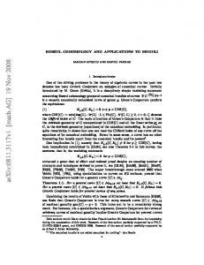
Let us consider the abelian monoid (Nn , +) of n-multi indices (or just multi indices when n is clear from the context) with addition defined componentwise. This can, on one side, be identified with the vertices of an n-dimensional integer lattice, and on the other side, with the abelian monoid of monomials in k[x1 , . . . , xn ] with the usual product, just by identifying the exponent of a monomial with the correspondent multiindex. Setting log(xµ ) = µ gives this correspondence. Given a set S of monomials, we say log(S) is just the set of all log(xµ ) with xµ ∈ S. Thus, the set of multiples of a given monomial xµ can be identified with the set µ + Nn = {µ + ν|ν ∈ Nn }. It is a monoid ideal. If we call this the span of µ in (Nn , +), then the set of monomials in the monomial ideal I = hxµ1 , . . . , xµr i can be identified with the union of the spans of its generators, and with the corresponding vertices in the n-dimensional integer lattice; we call this the lattice span of I. This union of spans is just log(I). In the low dimensional cases, where n equals 2 or 3, we can draw the lattice span of a given ideal I. These drawings are known as the two or three-dimensional staircase diagrams of monomial ideals and are useful tools for studying monomial ideals in two or three variables, see [MS04]. Their analogues in higher dimensions are also useful although obviously do not have such nice graphical representations. Figures 1.1 and 1.2 show some examples of staircase diagrams. In figure 1.1 the colored squares represent the multidegrees of the monomials inside the ideal I, whereas in figure 1.2 the colored cubes represent the multidegrees of the monomials not in I. In general, the correspondence of monomial ideals and monoid ideals in (Nn , +) allows us to interpret some relations and operations such as divisibility and multiplication in terms of addition or substraction of multi indices. This gives us a good tool to easily verify ideal membership of a given monomial or polynomial with respect to a monomial ideal, to compute least common multiples or great common divisors of sets of monomials, or even compute more complicated objects such as intersection of ideals,

14

Chapter 1

y3


x2 y 2

x3 Figure 1.1: Staircase diagram of I = hx3 , x2 y 2, y 3 i

z3

y3

x3

x2 y

Figure 1.2: Staircase diagram of I = hx3 , x2 y, y 3, z 3 i

1.2 Monomial Ideals

15

union, colon ideals... (for detailed descriptions see, for example [Bay96, MS04, MP01]). More explicitly: • A monomial xµ divides a monomial xν where µ = (µ1 , . . . , µn ) and ν = (ν1 , . . . , νn ) if and only if νi ≥ µi for all 1 ≤ i ≤ n. A monomial xν is in the ideal generated by {xµ1 , . . . xµr } if it is divisible by some generator. • The least common multiple of two monomials xµ and xν is the monomial lcm(xµ , xν ) = xρ with ρ = (max(µ1 , ν1 ), . . . , max(µn , νn )). The greatest common divisor of xµ and xν is the monomial gcd(xµ , xν ) = xσ with σ = (min(µ1 , ν1 ), . . . , min(µn , νn )). • If I = hxµ1 , . . . xµr i and J = hxν1 , . . . xνs i are monomial ideals, then we have that I +J = hxµ1 , . . . xµr , xν1 , . . . xνs i and I ∩J = h{lcm(xµi , xνj )|1 ≤ i ≤ r, 1 ≤ j ≤ s}i. • If I = hxµ1 , . . . xµr i is a monomial ideal and xν is a monomial not in I, then the quotient ideal (I : xν ) = {f ∈ R|f · xν ∈ I} is given by lcm(xµ1 , xν ) xµr lcm(xµr , xν ) xµ1 i=h ,..., ,..., i (I : x ) = h gcd(xµ1 , xν ) gcd(xµr , xν ) xν xν ν

In particular, xν is said to be regular for I if it is not a zerodivisor in R/I, if and only if (I : xν ) = I if and only if gcd(xµi , xν ) = 1 for all i, if and only if lcm(xµi , xν ) = xµi · xν for all i. So, for monomial ideals we have an easy way to characterize regular sequences (see the definition in appendix A). Another interesting object related to the combinatorial nature of monomial ideals is the lcm-lattice, see [GPW99]. Given a monomial ideal I minimally generated by {m1 , . . . , mr }, we denote by LI the lattice with elements labeled by the least common multiples of subsets of {m1 , . . . , mr } ordered by divisibility. We call LI the lcm-Lattice of I. The minimal element of this lattice is 1 (lcm of the empty set) and the maximal element is lcm(m1 , . . . , mr ). We will also denote by LI,i the subset of LI given by those elements labelled by the lcm of exactly i monomials in {m1 , . . . , mr }. Of course, S LI = i=0,...,r LI,i. As we have seen this lattice can be very easily translated into a subset of the integer lattice in n variables. The lcm-lattice LI will be very useful when discussing Hilbert series, Betti numbers and resolutions of monomial ideals, in particular the Taylor resolution (see later).

1.2.2

The algebra of monomial ideals

Many interesting algebraic objects associated with ideals of the polynomial ring have closed form expressions when we deal with monomial ideals. The following is a nonexhaustive list of the most relevant of these objects and/or those which will play some role on the subsequent chapters. Most definitions and properties in this section come from [MS04] and [Vil01]. For the definition of the several algebraic objects involved, see Appendix A.

16

Chapter 1

1.2.2.1


Prime, primary and irreducible monomial ideals.

Prime, primary and irreducible ideals (see appendix A) are particularly important classes of ideals. Their description, characterizations and some important properties can be easily obtained in the case of monomial ideals. Proposition 1.2.4. A monomial ideal is a prime ideal if and only if it is a face ideal i.e. it is generated by some set of variables. Proposition 1.2.5. A monomial ideal I is a primary ideal if and only if, after permutation of the variables, I has the form I = hxa11 , · · · , xar r , xb1 , . . . , xbs i, where ai ≥ 1 and ∪si=1 supp(xbi ) ⊂ {x1 , . . . , xr }, r ≤ n. In particular, the powers of face ideals are primary. Proposition 1.2.6. A monomial ideal I is irreducible if and only if up to permutation of the variables, I can be written as I = hxa11 , . . . , xar r i where ai > 0 for all i, r ≤ n. With these descriptions, some interesting properties about these ideals and decompositions of any monomial ideal in terms of special ideals are given. Some properties are more easily stated when speaking about squarefree monomial ideals, which are of great importance due to their relation with simplicial complexes, see [MS04, Sta78, Vil01]. Proposition 1.2.7. Let I be a monomial ideal of k[x1 , . . . , xn ] with k a field, then every associated prime of I is a face ideal. In the case of squarefree monomial ideals we even have the following relation: Corollary 1.2.8. If I is a squarefree monomial ideal and J1 , . . . , Js are the associated primes of I then I = J1 ∩ · · · ∩ Jn . Proposition 1.2.9. A monomial ideal I ⊂ R is squarefree if and only if any of the following conditions hold: 1. I is an intersection of prime ideals. 2. rad(I) = I 3. A monomial m is in I if and only if x1 · · · xr ∈ I, where supp(m) = {xi }ri=1 Proposition 1.2.10. Let I be a monomial ideal, then I has an irredundant primary decomposition I = J1 ∩ · · · ∩ Jr where Jk is a primary monomial ideal for all k and rad(Jk ) 6= rad(Jl ) if k 6= l. This proposition provides with an algorithm for computing minimal primary decompositions of monomial ideals (which need not to be unique), by successive elimination of powers of variables. A detailed description can be found in [Vil01].

1.2 Monomial Ideals

17

Proposition 1.2.11. If I is a monomial ideal, then there is a unique irredundant decomposition I = J1 ∩ · · · ∩ Jr such that every Ji is an irreducible monomial ideal. Remark 1.2.12. Irreducible components of monomial ideals are very closely related to the minimal generators of their Alexander duals. A complete description of the role of this beautiful duality when studying monomial ideals can be found in [MS04] and [Mil00], with several examples and other applications. We will meet Alexander duality in section 1.3.

1.2.2.2

Integral closure of monomial ideals.

Integral closures (see definition in Appendix A) have become an active area of research within commutative and computer algebra in the recent years (see for example [Vas05]) in the case of monomial ideals, again their combinatorial properties provide us with characterizations and description that makes this case easier to handle. First of all the following proposition states that the integral closure of a monomial ideal is a monomial ideal, and gives a description (cf. [Vil01, Cri02]). Proposition 1.2.13. Let I ⊂ R be a monomial ideal, then its integral closure I¯ is also a monomial ideal. We have that I¯ = hm|ml ∈ I l for some li With the help of the staircase diagrams we have seen in the precedent section and the correspondence provided by the log map, we can give a geometric description of the integral closure of a monomial ideal. For this description we need to recall the definition of the (rational) convex hull of a set of elements in the lattice Nn : Definition 1.2.14. Let µi = (µi1 , . . . , µin ) ∈ Nn , then its (rational) convex hull is conv(µ1 , . . . , µr ) =

( r X i=1

λi µi such that

r X

λi = 1, λi ∈ Q+

i=1

)

With this definition, we have Proposition 1.2.15. Let I be a monomial ideal, then the integral closure of I is given by I¯ = (xµ |µ ∈ conv(log(I)) ∩ Nn ) Example 1.2.16. Consider the ideal in R[x, y] given by I = hxy 15 , x3 y 10 , x6 y 5, x11 yi the ideal itself and its integral closure are depicted in figure 1.3. The integral closure of I is given by I¯ = hxy 15 , x2 y 13 , x3 y 10, x4 y 9 , x5 y 7 , x6 y 5 , x8 y 4 , x9 y 3, x10 y 2 , x11 yi In the picture, the new generators are drawn with white dots.

18

Chapter 1


xy 15

x3 y 10

x6 y 5

x11 y

Figure 1.3: The ideal I = hxy 15 , x3 y 10, x6 y 5 , x11 yi and its integral closure

1.2.2.3

Hilbert series of monomial ideals.

Hilbert series will be a central topic for us, since its study is closely related to that of resolutions; this relation is object of active research [Pee07]. Therefore, before going to the monomial case, we stop and give the basic general definitions. The Hilbert function and Hilbert series of a graded module of the polynomial ring are defined as follows: Definition 1.2.17. Let M be a graded R-module, the Hilbert function HM : Z → Z maps each integer z ∈ Z to the dimension as k-vector space of the degree-z piece of M, i.e. HM (z) := dimk (Mz ) The Hilbert series is defined as HSM(t) :=

X

HM (z) · tz

z∈Z

Through these pages, when it is clear from the context, we will use the notation HM alternatively for the Hilbert function and series. One main property of the Hilbert function, due to Hilbert himself is that the Hilbert function becomes polynomial for large z, thus the information in it can be expressed in a simple way: Theorem 1.2.18. If M is a finitely generated graded R-module then HM (z) agrees for large z with a polynomial of degree ≤ n.

1.2 Monomial Ideals

19

Definition 1.2.19. This polynomial is called the Hilbert polynomial of M and is denoted by HP (t). Consider now an exact sequence of graded R-modules, 0 → Mk → · · · → M0 → 0 using the rank nullity theorem from linear algebra, we have that HSMk =

k−1 X

(−1)i HSMi

i=0

This fact provides us a good tool for the computation of Hilbert series, and even a way to proof theorem 1.2.18, see [Eis95] for example. Another crucial result for computing Hilbert series is the fact that for any degreepreserving monomial ordering defined in R (see definition of monomial orderings in appendix A) and any ideal I of R, we have that the Hilbert series of I and lt (I) coincide; thus, we can reduce the computation of these Hilbert series to computations on monomial ideals. In the case of multigraded modules, we can define a multigraded version of these objects. Multigraded (or Nn -graded) R-modules are those modules M such that M = ⊕a∈Nn Ma and xa Mb ⊆ Ma+b a, b ∈ Nn . In this case, one can define the multigraded Hilbert series as X dimk (Ma ) · xa . HM (x) = a∈Nn

Monomial ideals are a particular case of multigraded R-modules.

Remark 1.2.20. The multigraded Hilbert series is an element of the formal power series 1 ring Z[[x1 . . . , xn ]] and in this ring we have that 1−x = 1 + xi + x2i + · · · . Since the i multigraded Hilbert series of R is just the sum of all monomials in R, we have HR (x) = Qn 1 . If we shift the grading of R by a, i.e. consider the free module generated in i=1 1−xi multidegree a, which we will denote R(−a), it is isomorphic to hxa i, then HR(−a) (x) = xa xa · HR (x) = 1−x . i If I is a monomial ideal, then the multigraded Hilbert series of the R-module R/I is just the sum of all monomials not in I. Remark 1.2.21. Multigraded Hilbert series of monomial ideals and modules of the form R/I for I a monomial ideal, can be expressed as rational functions of the type HM (x) =

KM (x) (1 − x1 ) · · · (1 − xn )

the numerator KM (x) is known as the K-polynomial of M, see [MS04]. Most of the time we will be interested in computing the K-polynomial of some ideal or some module R/I. It is easy to see that if I is a monomial ideal, KR/I (x) = 1 − KI (x).

20

Chapter 1


When computing the multigraded Hilbert series of a monomial ideal I, one can use the lcm-lattice in the following way: We need to ‘count’ the monomials in I, and we have seen that the multigraded Hilbert series i.e. the sum of all the monomials in an ideal a generated by a single monomial xa is of the form Hhxa i (x) = xa · HR (x) = Qn x(1−xi ) , i=1 so we need to sum these factors for each of the generators of our ideal. But doing so, we would add too many times some of the monomials in I, those belonging to the span of more than one generator. To avoid this, we can delete to our sum the corresponding factors of the pairwise intersections of the spans of the generators. These intersections are just ideals generated by the pairwise lcm’s. Again, deleting all these, would delete too many times the monomials belonging to more than one of such new ideals, and so on... Thus, we need to perform an inclusion-exclusion procedure, that leads us to the following formula for the multigraded Hilbert function of I in terms of the lcm-lattice LI : Pn P i−1 a i=1 (−1) xa ∈LI,i x HI (x) = (1 − x1 ) · · · (1 − xn ) where LI,i is the set of the lcm’s of sets of i generators of I. If we call KLI (x) to the numerator in this formula, before performing any cancellations among the factors, then we have that 1 − KLI (x) HR/I (x) = . (1 − x1 ) · · · (1 − xn ) Example 1.2.22. Consider the ideal I = hx2 , xy, y 2, yzi; its lcm-lattice LI is formed by: LI,1 = {x2 , xy, y 2, yz}, LI,2 = {x2 y, x2 y 2, x2 yz, xy 2 , xyz, y 2z}, LI,3 = {x2 y 2 , x2 yz, x2 y 2z, xy 2 z} and LI,4 = {x2 y 2z} thus, we have KLI (x) = x2 +xy+y 2+yz−(x2 y+x2 y 2+x2 yz+xy 2 +xyz+y 2 z)+(x2 y 2+x2 yz+x2 y 2z+xy 2 z)−x2 y 2 z after cancellation of terms, we obtain KI (x) = x2 + xy + y 2 + yz − x2 y − xy 2 − xyz − y 2 z + xy 2 z The lcm-lattice produces as we have seen a closed formula for the K-polynomial, but in general it contains much too many terms. Better formulas can be obtained from free resolutions of the ideal, in particular from the minimal free resolution and Betti numbers, as we see in the next paragraph.

1.2.3

Homological invariants of monomial ideals

We shall pay special attention to the homology of monomial ideals and its related invariants. The main object here are resolutions. Among them, a special object is the minimal resolution and the ranks of the modules forming it, i.e. the Betti numbers. The fact that monomial ideals are multigraded modules, allows us to obtain multigraded resolutions. This multigrading will be very useful from both the theoretical and computational viewpoints.

1.2 Monomial Ideals 1.2.3.1

21

Free resolutions, Betti numbers and Betti multidegrees.

Given an R-module M, a resolution of it is a complex P of free modules that is exact everywhere except at dimension 0 in which we have H0 (P) ≃ M (see Appendix A for the necessary definitions). A well known result by Hilbert states that every finitely generated graded R-module has a free resolution of length at most n. Among all the possible resolutions of a graded module, a special role is played by the minimal one, which is unique up to isomorphisms. The ranks of the modules in the minimal resolution are called the Betti numbers of M and are the most important homological invariants of an R-module. As we have seen for the Hilbert series, the fact that monomial ideals are multigraded modules, leads to some extra properties. In the case of free resolutions, the main one is that free resolutions of multigraded modules, are also multigraded. When taking into δ δ account the multigrading of a resolution P : · · · Pi →i Pi−1 → · · · → P1 →i P0 → 0, we will consider the fact that the free modules Pi are Nn -graded and each homomorphism δi is multidegree preserving. In the case of minimal resolutions of Nn -graded modules, we L βi,a have that Pi = a∈Nn R (−a) then, we define the i-th Betti number of the multigraded module M in multidegree a is the invariant βi,a = βi,a (M); we will consider only those which are not zero. These are what we will call multigraded Betti numbers. Being I a monomial ideal, we have that the βi,a (I) measure the number of minimal generators required in multidegree a for the i-th syzygy module of I. We note that they can also be characterized by means of Tor since the i-th Betti number of an Nn -graded R module M in degree a equals the vector space dimension dimk T ori,a (M, k). It will be useful to collect the multidegrees in which the multigraded Betti numbers are non-zero: Definition 1.2.23. Let M be a multigraded R-module. Let us denote by B(M) the set of multidegrees in which the multigraded T or modules are nonzero: B(M) = {a ∈ Nn |T ori,a (M, k) 6= 0 for some i} We call B the set of Betti multidegrees of I. The corresponding sets Bi (M) = {a ∈ Nn |T ori,a (M, k) 6= 0} are called the i-th Betti multidegrees of M. Equivalently, the Betti multidegrees are defined to be those multidegrees in which the multigraded Koszul homology of M does not vanish i.e. those in which the multigraded Betti numbers are different from zero. When a given multigraded Betti number is bigger than one, it will sometimes be useful to consider that multidegree as appearing repeated among the Betti multidegrees, then we speak of the collection of Betti multidegrees to take these eventual repetitions into account. Remark 1.2.24. Given an ideal I considered as an R-module, it can be described using a free resolution, and the same can be done with the module R/I. Both of them are very

22

Chapter 1


related and the information provided for their respective resolutions is equivalent, as is the information given by the Koszul homology of I and R/I. The reason is the following: If we have a resolution P of I of the form δ

δ

P : · · · Pi →i Pi−1 → · · · → P1 →i P0 → 0 then we have a resolution of R/I δ

δ

P : · · · Pi →i Pi−1 → · · · → P1 →i P0 → R → 0 and then for all i, we have βi (I) = βi+1 (R/I) and also for the multigraded Betti numbers: βi,a (I) = βi+1,a (R/I) ∀a ∈ Nn . Moreover, we have that Hi (K(I)) ≃ Hi+1 (K(R/I)) and the isomorphism preserves multidegree. Thus, from a theoretical point of view it is almost equivalent to work with I or with R/I. Sometimes it is more convenient to work with resolutions of R/I, in particular in the theoretical settings, because some of the concepts are more clear and easy to handle, and it is the most frequent framework in the literature. On the other hand, sometimes is more convenient to work with I and its Koszul complex, because then we can handle the monomials directly, not their equivalence classes modulo I, and the generating sets of the Koszul modules can be expressed in a simpler way. In order to recover all the information about R/I from the information over I or vice versa, we need explicit isomorphisms between the Koszul homology modules of R and R/I. This is provided by the Spencer differential, in particular observe that if µ is a generator of the i-th Koszul homology group of I then δ(µ) is a generator of the i + 1-st Spencer cohomology group of R/I (see section 1.1.4), i.e. the corresponding multidegrees are identical. Therefore, we will speak alternatively of I or R/I. Most of the time, we will use R/I in the theoretical part when speaking about resolutions, and we will use I when giving explicit formulas or in Koszul homology computations. Multigraded resolutions are very closely related to multigraded Hilbert functions, as the following proposition (which is an easy consequence of the rank-nullity theorem) shows: Proposition 1.2.25. Let P be a multigraded resolution of the monomial ideal I and let mi,α the rank of the multidegree α component of the module Pi in the resolution. Then the K-polynomial of I is given by X KI (x) = (−1)i−1 mi,α xα i>0,α∈N

in case P is the minimal resolution, we have X (−1)i−1 βi,α xα KI (x) = P

i>0,α∈N

We will denote KP (x) the formula i>0,α∈N (−1)i−1 mi,α xα before performing any cancellations, and call it the K-polynomial of I in terms of P.

1.2 Monomial Ideals

23

In terms of the Betti multidegrees, we have that KI is the alternating sum of the Bi (I) in which every multidegree a is counted βi,a (I) times. In order to avoid too many redundant terms and cancellations in the form we obtain for KI from resolutions, we will prefer smaller resolutions, and the less redundant one is the minimal resolution: Proposition 1.2.26. Let I be a monomial ideal and let P be a free resolution of I; let M be the minimal free resolution of I. Any terms that can be cancelled in KM (x) can also be cancelled in KP (x). Proof: If a term of multidegree a can be cancelled in KM (x) then we have that a belongs to Bi (I) and Bj (I) with i 6= j each of them having different parity. In other words, the multidegree a pieces of Mi and Mj , namely Mi,a and Mj,a have positive rank. Since by definition of minimal resolution and since the free resolutions of I are multigraded, we have that the rank of Pk,b is bigger or equal to the rank of Mk,b for every k and b then Pi,a and Pj,a have positive rank and hence the same cancellation is possible in KP (x) 1.2.3.2

Examples of monomial resolutions

The efficient computation of minimal resolutions is a difficult task, even in the monomial case [BPS98, GPW99], for which no general closed formula has been given. Research in this field has led to define on one hand non-minimal resolutions of general monomial ideals [Tay60, Lyu98], and in the other hand, to study special classes of monomial ideals for which their minimal resolutions can be explicitly given or at least easily computed [EK90, MS04]. Probably the best known resolution of a monomial ideal is Taylor’s resolution [Tay60], which has a very simple explicit description. In general, Taylor resolution is highly nonminimal. A subresolution of Taylor’s is Lyubeznik resolution [Lyu98], still nonminimal. There are a number of other nonminimal resolutions in the literature cited in the references (for instance, a resolution of minimal length for some types of ideals is described in [Sei07b]), here we shall describe only cellular resolutions [MS04], and in particular the Scarf resolution, which is minimal for a special family of monomial ideals, called generic ideals. More recently discrete Morse theory has also been applied to the study of resolutions of monomial ideals [Bat02, OW07] Taylor and Lyubeznik resolutions: Let I be a monomial ideal and {m1 , . . . , mr } a generating set of I. For any subset J = {j1 , . . . , js } ⊆ {1, . . . , r}, let us denote mJ = lcm(mj1 , . . . mjs ),and J i = {j1 , . . . , jbi , . . . , js }. We can construct a resolution of R/I in the following way: Let Ts , s ≥ 0 be a free R-module generated as a vector space by the set {uJ s.th. |J| = s} and consider the R-linear differential X mJ d(uJ ) = (−1)i−1 uJ i mJ i i∈J

24

Chapter 1


it is easy to verify that d2 = 0. Moreover, this complex is acyclic and it is a resolution of R/I. This resolution is due to D.Taylor [Tay60] and will be denoted by T = (Ti , di ). The length of Taylor’s resolution is given by the number of elements in the given generating set of the ideal (normally, we will assume we have a minimal generating set for the ideal), r which we denote by r. The rank of the i-th free module Ti is i , thus the sum of all these ranks, i.e. Size(T) is 2r . Remark 1.2.27. Generally, Taylor’s resolution is far from minimal, although [Bat02] gives the following condition for a monomial ideal to be minimally resolved by Taylor’s resolution: Let I be a monomial ideal, then the Taylor resolution of I is minimal if and only if for all J in the support of T(I) and all m ∈ J we have m ∤ lcm(J r {m}). Other characterizations of monomial ideals for which the Taylor resolution is minimal are given by Fröberg [Fro78] and Herzog et al. [HHMT06] A subresolution L of T was given in [Lyu98] and it is known as the Lyubeznik resolution. It is defined as follows: For a given subset J ⊆ {1 . . . r} and an integer 1 ≤ s ≤ r, let J>s = {j ∈ J|j > s}; then L is generated by those basis elements uJ such that for all 1 ≤ s ≤ r one has that ms does not divide mJ>s . It is clear that, unlike Taylor’s, Lyubeznik resolution depends on the ordering in which the generators of the ideal are given. Example 1.2.28. Let us consider the following monomial ideal in three variables: I = hx2 y, xy 3, xz, yzi, the Taylor resolution T(I) of I has length 4, size 16 and the differentials are given by

x2 y xy 3 xz yz

d1 = 

   d3 =    

 −z −z 0 0 y2 0 −1 0   0 y2 1 0   −x 0 0 −1   0 −x 0 1  0 0 −x y 2



 y2 z z 0 0 0  −x 0 0 z z 0   d2 =  3  0 −xy 0 −y 0 y  0 0 −x2 0 −xy 2 −x 

 1  −1   d4 =   y2  −x

Lyubeznik’s resolution is in this case equal to Taylor’s if we keep the ordering m1 = x2 y, m2 = xy 3 , m3 = xz, m4 = yz. On the contrary if we change the order to m1 = xz, m2 = yz, m3 = x2 y, m4 = xy 3 , then L is generated by u1 , u2 , u3 , u4 , u12 , u13 , u14 , u34 and u134 i.e. the size of L is 10. In this case, L is minimal. The differentials are given by

δ1 =



  y2 z 0 0 −z 2    −x 0 z 0  δ3 =  y xz yz x2 y xy 3 δ2 =   0 −xy −y 3 y   −x 0 0 0 −x 0

   

1.2 Monomial Ideals

25

Remark 1.2.29. In [Sei02b] Taylor and Lyubeznik resolutions are described in relation with the Buchberger algorithm for the construction of Gröbner bases. Taylor resolution is shown to be obtained by repeated application of the Schreyer theorem from the theory of Gröbner bases, and the Lyubeznik resolution is shown to be a consequence of Buchberger’s chain criterion. The Taylor resolution is strongly related to the lcm-lattice of a monomial ideal (see [GPW99]). If we consider Taylor’s resolution of R/I, we see that all the multidegrees of the generators lie in LI . Then, applying a minimization process to this resolution, to obtain a minimal one (as described for example in [CLO98] or the reduction algorithm described below) we have that no new multidegrees will appear, although some can eventually disappear. Thus, this is a simple way to show that βi,a (I) = 0 if a ∈ / LI . Cellular resolutions: In the thesis [Mil00] and their book [MS04], E. Miller and B. Sturmfels define and give some interesting properties and families of what they call cellular resolutions. These are a type of geometrical resolutions that can be associated to monomial ideals. Here we will only repeat some of the basic definitions, for deeper details we point the interested reader to the original source. A useful tool to handle monomial resolution are monomial matrices: Definition 1.2.30. A monomial matrix is an array of scalar entries λqp whose columns are labeled by source degrees ap , whose rows are labeled by target degrees aq , and whose entry λqp ∈ k is zero unless ap ≥ aq . In the usual unlabeled notation, the entry λqp is replaced by λqp · xap −aq . Definition 1.2.31. A polyhedral cell complex X is a finite collection of convex polytopes (in a real vector space Rm ) called faces of X, satisfying two properties: • If P is a polytope in X and F is a face of P, then F is in X • If P and Q are in X, then P ∩ Q is a face of both P and Q Definition 1.2.32. X is a labeled cell complex if its r vertices have labels that are vectors a1 , . . . , ar in Nn and the label on an arbitrary face F of X is the exponent aF on the least common multiple lcm(xai |i ∈ F ) of the monomial labels xai on vertices in F . Definition 1.2.33. Let X be a labeled cell complex. The cellular monomial matrix supported on X uses the reduced chain complex of X for scalar entries, with ∅ in homological degree 0. Row and column labels are those on the corresponding faces of X. The cellular free complex FX supported on X is the complex of Nn -graded free R-modules (with basis) represented by the cellular monomial matrix supported on X. The free complex FX is a cellular resolution if it is acyclic (homology only in degree 0).

26

Chapter 1


Remark 1.2.34. Observe that Taylor resolution is an example of cellular resolution. In this case, X is the full (r − 1)-simplex with the r vertices labeled by the exponents of the generators of I. Several examples of cellular resolutions can be found in [MS04], like those for permutohedron ideals, tree ideals, etc. Of particular importance is the hull resolution, which is a canonical construction of a resolution of length less than or equal n, which is generally nonminimal. An important family of monomial ideals for which the hull resolution is not only minimal but also has a simple description is that of generic monomial ideals: Definition 1.2.35. A monomial ideal hm1 , . . . , mr i is generic if whenever two distinct minimal generators mi and mj have the same positive (nonzero) degree in some variable, a third generator mk strictly divides their least common multiple lcm(mi , mj ) Definition 1.2.36. let I be a monomial ideal with minimal generating set {m1 , . . . , mr }. The Scarf complex ∆I is the collection of all subsets of {m1 , . . . , mr } whose least common multiple is unique: ∆I = {σ ⊆ {1, . . . , r}|mσ = mτ ⇒ σ = τ } The Scarf complex is a simplicial complex of dimension at most n − 1 and the chain complex supported on it, the algebraic Scarf complex F∆I , is included as a subcomplex in any resolution of I. For generic monomial ideals, the Scarf complex provides the minimal resolution, thus, the minimal resolution of these ideals is simplicial: Theorem 1.2.37. If I is a monomial ideal, then its Scarf complex ∆I is a subcomplex of the hull complex hull(I). If I is generic then ∆I = hull(I) so its algebraic Scarf complex F∆I minimally resolves I. Example 1.2.38. The ideal in example 1.2.28 is not generic. Its Scarf complex is formed by the sets {{1}, {2}, {3}, {4}, {12}, {34}} and its algebraic counterpart is not a resolution of I. Remark 1.2.39. In the non-generic case, the Scarf complex can be perturbed to obtain another complex with supports a resolution of I which is non-minimal in general. A simple description of this perturbation procedure can be seen for example in [GW04]. 1.2.3.3

Minimizing resolutions

To close this section on free resolutions we refer to the fact that the minimal resolution of an ideal I is contained as a subcomplex in every resolution of I. Given some resolution, there are explicit algorithmic ways to reduce it until obtaining the minimal resolution. Inside Theorem 3.15 in [CLO98] a procedure to simplify a given graded resolution is described. Here we give a simple equivalent description of this process, based on the Chain Complex Reduction Algorithm (CCR). This algorithm is applied in general to

1.2 Monomial Ideals

27

chain complexes and has a geometric interpretation in the case of simplicial, cubical or CW-complexes. A description of it can be found in [KMM04]. We give here first the basic definitions and theorems in which the algorithm is based. After this we apply these results to the case of resolutions of monomial ideals. Definition 1.2.40. Given a free chain complex {C, δ}, we say that two chains c ∈ Ci ′ and c′ ∈ Ci+1 are a reduction i has an inverse, where Pm pair if hδ(c), cP Pm h·, ·i denotes their m scalar product hc1 , c2 i := i=1 αi , βi if c1 = i=1 αi ei and c2 = i=1 βi ei

Assume we have a generator c of the module Ci−1 and a generator c′ ∈ Ci that form a reduction pair in some chain complex {C, δ}. Using this information, we want to define ¯ whose basis is a subbasis of {C, δ}. Let Wk denote the set ¯ δ} a new chain complex {C, of generators of Ck . Say Wi = {b1 , . . . , bdi , b} and Wi−1 = {a1 , . . . , adi−1 , a}, being (a, b) ¯ i = {b1 , . . . , bd } and W ¯ i = {a1 , . . . , ad } and W ¯ j = Wj for a reduction pair. Define W i i−1 all other j. The new differential δ¯ is defined with the following formulas for every chain in C:  hδ(c),ai  δ(c) − hδ(b),ai δ(b) if j = i δ¯j (c) = δ(c) − hδ(c), bib if j = i + 1  δ(c) otherwise

Observe that in this formula the condition of hδ(b), ai having an inverse is required (which is relevant in case our coefficients do not lie on a field). With this formula, we have that

¯ and the isomorphism is induced in homology by the Theorem 1.2.41. H∗ (C) ≃ H∗ (C) projection π ¯ , which can be expressed by the following explicit formula:  hc,ai  c − hδ(b),ai δ(b) if j = i − 1 π¯j (c) = c − hδ(c), aib if j = i  c otherwise

This projection is the mathematical expression of the reduction step performed in the original complex via the reduction pair (a, b). The idea of the CCR algorithm is to perform these reduction steps while possible, resulting in each step a smaller complex with the same homology as the original one. The size of the corresponding complex is reduced by two on each reduction step.

In our case, given a monomial ideal I ⊆ k[x1 , . . . , xn ], we describe a free resolution by giving a sequence of modules with their generators, and a sequence of matrices that describe the differentials. Recall that given a free resolution of a monomial ideal, it is minimal if and only if it has no nonzero constant polynomials in the entries of the matrices describing the differentials in the complex. Starting with some non-minimal resolution P of I, whenever we have a nonzero constant entry c in one of the matrices in the complex, say in the column that expresses the differential applied to generator e′ ∈ Pi+1 at the row corresponding to generator e ∈ Pi then clearly hδ(e), e′ i = c thus, for every nonzero scalar in a differential, we have a reduction pair and we can apply

28

Chapter 1


the standard result described above and we obtain a smaller complex that is still a resolution. It is clear that no new constant terms will be added in this step, thus, after applying the reduction step we have seen for chain complexes, we have a smaller chain complex which the same homology as P (i.e. it is still a resolution of I) and has both smaller size and less constant terms in the differentials. Thus performing this reduction successively, we will reach a resolution with no constant terms in the differentials, i.e. the minimal resolution.

1.3

Topological and homological techniques for monomial ideals

In this section we give a collection of topological and homological techniques applicable in the study of monomial ideals. Since we are focused on the multigraded homological description of monomial ideals, which can be summarized by the multigraded T or modules the multigraded minimal resolution and the Betti numbers, the techniques we will explore have this homological flavour. On the other hand, the combinatorial nature of monomial ideals suggests the use of combinatorial techniques. Thus, the first objects that will appear in our collection are simplicial complexes, a distinguished area where homology meets combinatorics. The connection between simplicial complexes and Betti numbers of monomial ideals has been applied among others by Hochster [Hoc77], Stanley [Sta96], Burns and Herzog [BH97], Eagon and Reiner [ER98], Bayer [Bay96] or Miller and Sturmfels [MS04]. The simplicial Koszul complex, introduced by the latter authors, will be our first object, after which we introduce Stanley-Reisner ideals and relate them to Koszul simplicial complexes. Later on we shall move to exact sequences and will explore the Mayer-Vietoris sequence and its application to monomial ideals, as well as the algebraic mapping cone applied to resolutions of monomial ideals. All the objects in this section share their algorithmic capabilities. Our interest in actual computations is clearly fulfilled by the techniques we present here. Some of the techniques in the following pages were presented in [S06a]. Remark 1.3.1. There are a number of simplicial complexes that have been used to compute multigraded Betti numbers of monomial ideals, we focus here on the simplicial Koszul complex, other simplicial constructions can be seen in [BH97, BS98, GPW99, Pee02].

1.3.1

The simplicial Koszul complex

Simplicial complexes are well known objects that play an essential role in combinatorial algebraic topology. All the necessary definitions are given in Appendix B. One way to compute the Betti numbers or Koszul homology of I at a given multidegree a is to associate a particular simplicial complex to the ideal and the multidegree and express the Koszul homology of I at a in terms of this simplicial complex. This idea is presented

1.3 Topological and homological techniques for monomial ideals

29

in [Bay96], [Pee02] or [MS04] and also in [BH97] and in some sense gives a simplicial meaning to the contribution of each multigraded piece of the homological structure of a monomial ideal. Upper and lower simplicial Koszul complexes Definition 1.3.2. Let I be a monomial ideal, a = (a1 , . . . , an ) ∈ Nn and xa ∈ I. Let l = |support(a)| i. e. l is the number of nonzero components of a. We associate to a the l-simplex ∆a , where the vertices are labeled by the variables in the support of a. Now, we build the subcomplex of ∆a given by ∆Ia := {τ ∈ ∆a |xa /xτ ∈ I} where xτ is a squarefree monomial with exponents given by the variables defining the face τ . This is what is called the upper Koszul simplicial complex, in few words, it is described as ∆Ia = {squarefree vectors τ |xa−τ ∈ I} With this definition we have the following result that relates the simplicial homology of the upper Koszul simplicial complex to the multidegree a Betti numbers of I and hence with the multidegree a piece of the Koszul homology of I, see [Bay96, MS04]. Theorem 1.3.3. e i−1 (∆Ia ) ∀i Hi (K(I)a ) ≃ H

Proof: The proof is based on the fact that the corresponding chain complexes are equal under the isomorphism that maps an element in Kj (I) to a face of ∆Ia . Since this isomorphism between the chain complexes is compatible with the differentials we have the isomorphism in homology. Remark 1.3.4. The correspondence of the chains of the chain complex associated to ∆Ia with chains of K(I)a that makes explicit this isomorphism is just the k-linear extension of the correspondence that associates the face τ ∈ ∆Ia with xa /xτ ⊗ x(τ ) where, if τ = aτ1 , . . . aτk the exterior part (i.e. the right-hand side with respect to the tensor symbol) of the latter has to be understood as x(τ ) = xaτ1 ∧ · · · ∧ xaτk . Dual to the upper Koszul simplicial complex, we can define the lower Koszul simplicial complex in the following way, [Bay96, MS04]: Definition 1.3.5. For a ∈ Nn define a′ by subtracting 1 from each nonzero coordinate of a. The lower Koszul simplicial complex of I at a is given by ′

∆aI = {squarefree vectors τ a|xa +τ ∈ / I}

30

1.3.2

Chapter 1


Simplicial computation of Koszul homology

Koszul simplicial complexes defined at each a ∈ Nn together with the fact that βa (I) = 0 if a ∈ / LI (recall LI is the lcm-lattice of I) provide us with a method of computing the Koszul homology of I in a finite number of steps. Namely, for each multidegree in the lcm-lattice of I (which is a finite set), we construct the corresponding upper or lower Koszul simplicial complex, and compute the corresponding singular homology. Thus, Koszul homology is computable for any monomial ideal. This way of computing Koszul homology can be expressed as an algorithm, it is shown in table 1.1. Algorithm : Naive Koszul Homology of a Monomial ideal I Input : Minimal generating set of I = hm1 , . . . mr i Output : Generators of the Koszul homology of I

1 2 3 4 5 6

Compute the lcm-lattice of I foreach a ∈ LI do Build the simplicial complex associated to a, ∆Ia Compute the reduced homology of ∆Ia endforeach returnH(K(I))∗ Table 1.1: Algorithm Naive Koszul Homology

The problem of this algorithm is its high complexity. The number of multidegrees in LI is bounded above by 2r and in some cases this bound will be reached, so we are dealing with an exponentially growing set of points in the lattice. On the other hand, at each of these points, we want to explicitly compute the reduced homology of a simplicial complex in n vertices, and this computation depends exponentially on the number of variables n. So the algorithm complexity is double exponential in n and r. Improvements of this algorithm must then focus in both reducing the number of relevant multidegrees for the computation and stressing the properties of monomial ideals in order to simplify the simplicial computations required at each multidegree. Both ways of improvements will be developed in the next paragraphs. We have just seen that the problem of computing the Koszul homology of I at a given multidegree is equivalent to the computation of the reduced homology of a subcomplex of an n-simplex. Since we want to explicitly compute these reduced homology modules, our problem reduces to compute quotients between the kernels and image subspaces of some matrices with coefficients in k. The most usual way to do this is via linear algebra algorithms keeping track of the generators of the corresponding modules, in particular Smith normal form algorithms. As our coefficients lie on a field, we can substitute Smith normal form computations with Gaussian elimination, which is more efficient in our case,


31

but we still have high complexity. Being this a hard problem in general, we can take advantage of several facts that will drastically improve our computations:

Computing homology dimension by dimension Instead of computing Koszul homology by exploring the whole lcm-lattice at once, we can proceed dimension by dimension. For the zero dimensional Koszul homology, we know that the generators are just the minimal generators of the ideal. In each subsequent dimension, we start with a candidate set of multidegrees in which we will eventually have non-vanishing Koszul homology. The actual candidate sets used are a subset of LI : we use as candidate set of multidegrees for dimension i, the least common multiples of pairs of multidegrees with non-vanishing homology in dimension i − 1. The reason to do this is that in a syzygy resolution of I, if I is monomial, and we have a minimal generating set of the (i − 1)-th syzygy module, then we can construct a generating set of the next syzygy module such that the multidegree of the new generators are least common multiples of pairs of the former ones. The multidegrees of the minimal generating set of syzygies for the new module will be of course a subset of these. And finally, the multidegrees of the elements in a minimal generating set of the i-th syzygy of I module coincide with the multidegrees in which the i-th Koszul homology of I does not vanish, for in both cases they are the multigraded Betti numbers. As in each step we obtain the multidegrees of the non-zero Betti numbers, we can use this information for building the set of candidate multidegrees for the next step. This procedure, on one hand reduces the number of multidegrees to be considered, for we don’t need to explore all the lcm-lattice, and on the other hand, it also reduces the complexity of the simplicial complexes for which we have to compute reduced homology: For each complex we only need to compute homology at a given dimension. For this we will only need a short part of the chain complex (C• , δ) associated to ∆Ia , namely, for computing the reduced homology in dimension i, we need the generators of Ci+1 , Ci and Ci−1 and the matrices defining δi+1 and δi . Now, for our purposes it is enough to consider a subcomplex of ∆Ia : given i, let us denote by ∆Ia,i the subcomplex of ∆Ia whose facets (i.e. the maximal faces) are the i + 1 and i-faces of ∆Ia , note that a simplicial complex can be completely described by fi (∆I ). Using these smaller fi (∆I ) = H giving its facets. Then it is easy to see that H a,i a complexes, the size of the needed matrices becomes smaller and we can reduce the size of our computations.

Example 1.3.6. Consider for example the ideal I = hxyzts, xytu, xyzu, xysu, tsui in the ring R = R[x, y, z, t, s, u] . If we take a = (1, 1, 1, 1, 1) then figure 1.4 shows ∆Ia and ∆Ia,2 . We can see in it that ∆Ia,2 is contractible, and thus H3 (K(I))a = 0.

32

Chapter 1 x


t

x

y

s

y

u z ∆Ia

z ∆Ia,2

Figure 1.4: The simplicial complexes ∆Ia and ∆Ia,2 for a = (1, 1, 1, 1, 1, 1).

Improvements based on simplicial homology An impressive amount of work has been done on the computation of the homology of simplicial complexes. Two main sources of improvement have been developed. On one side, one can improve the techniques for the computations needed on the matrices defining the differentials. Since these matrices have a big degree of sparsity, several techniques for dealing with Smith normal form algorithms and Gaussian elimination in the case of sparse matrices have resulted in fast algorithms for performing these computations [DER97, DSV01]. The second source comes from considerations on the simplicial complexes themselves. Here we will just make two simple considerations on the simplicial complexes we deal with, which can be used to improve our computations. In first place, sometimes it is easy to detect whether some homology groups vanish or not, without actually compute them. In particular it is easy to detect if ∆Ia is the full lsimplex (where l = |supp(a)|), and thus contractible: we just check if xa−(0,...,1i1 ,...,1il ,...,0) is in the ideal I, this is performed just by monomial divisions. If it is the case, we know that H∗ (K(I)) vanishes at a. On the other hand we can also easily check whether all the (i + 1)-faces of the l-simplex are present in ∆Ia or not. If it is the case, then ∆Ia,i is contractible, and thus the Koszul homology of I in dimesion i vanishes at a; this is also easy to check. To illustrate these facts we see in table 1.2 a comparison between the number of elements of the lcm-lattice LI , the size of the Taylor resolution, the number of noncontractible Koszul simplicial complexes and the size of the minimal resolution for some random examples. In the table, n denotes the number of variables, g the number of generators, md the minimal degree of a generator, and Md the maximal degree of a generator. We can see how the simple considerations just exposed produce a severe reduction in the number of complexes to be considered.


33

n

g

Md/md

lcm-lattice

Taylor

non-contractible

Minimal

3 3 6 6 9 9

5 12 5 12 7 8

56/26 57/28 128/45 114/60 168/73 176/101

20 158 26 467 75 157

32 4096 32 4096 128 256

12 48 19 225 43 111

11 45 19 169 37 103

Table 1.2: Number of non-contractible complexes, compared with lcm-lattice and Taylor and Minimal resolutions

Remark 1.3.7. In [Rou07], the following simplicial complex is defined: AI := {M ⊂ min(I)|π(lcm(M)) ∈ / I} 1 ···xn ) . Observe where min(I) is the set of minimal generators of I, and π(m) = lcm(m,x x1 ···xn that the multidegrees of the faces of AI are exactly those that we have eliminated using the above criterion, i.e. the numbers in the column non-contractible in table 1.2 are the number of different multidegrees of the faces of AI . The complex AI supports a simplicial resolution of I, which is a subresolution of Taylor’s, the size of which is bounded below by the numbers under the non-contractible column in table 1.2

Remark 1.3.8. This is yet another easy proof of the fact that the Koszul homology of I vanishes at all multidegrees not in the lcm-lattice LI , because if a is not in LI then either ∆Ia is empty (if a ∈ / I) or it is the full l-simplex (if a ∈ I); in both cases, the homology vanishes. Remark 1.3.9. We can also use dualities to improve our computations. The simplicial version of Alexander’s duality is in particular useful for our purpose, see[Bay96, MS04]. The Alexander Dual of a simplicial complex given by a collection S of subsets of the n-simplex ∆ is given by S ∨ = {F |F c ∈ / S} = {F |F ∈ / S c} fi (S) ≃ where c denotes set complementing. The Alexander duality theorem states that H n−i−3 ∨ i ∨ e e (S) ≃ H e n−i−3 (S ). Thus, depending on the size of our complex inside H (S ) and H the l-simplex, it is sometimes better from the computational point of view, to compute in the Alexander dual of ∆Ia . Some other forms of duality can also be of interest for further improvements. With the considerations made above, we can make several improvements to our first naive algorithm for compute the Koszul homology of a monomial ideal. Using topological and algebraic arguments, we can reduce the number of corners in which we have to actually perform these computations, moreover, these computations are improved and we only compute the homology of the resulting simplicial complexes at the particular dimensions we need.

34

Chapter 1


Algorithm : Dimension-by-dimension Koszul Homology of a Monomial ideal I Input : Minimal generating set of I : {m1 , . . . mr } Output : Generators of the Koszul homology of I

1 2 3 4 5 6 7 8 9 10 11 12 13 14 15 16 17 18 19

H0 (K(I)) =< m1 , . . . , mr > S ← {multideg(m1 ), . . . , multideg(mr )} i := 1 while i < n and |S| > 1 do lcm(S) ← {lcm(sk , sj )|sk , sj ∈ S} S = {}, Hi (K(I)) = {} foreach sk,j ∈ lcm(S) do if Not is-contractible(sk,j ) then Build (∆Isk,j )i ˆ i ((∆Is )i ) Compute H k,j ˆ i ((S I )i ) 6= 0 then if H sk,j S ← S ∪ sk,j ˆ i (∆I ) H(K(I))i ← H sk,j endif endif endforeach i=i+1 returnH∗ (K(I)) endwhile Table 1.3: Algorithm Dimension-by-dimension Koszul Homology

The improved algorithm can be seen in table 1.3. Observe that in line 9 we use a subroutine Build that builds the part of the chain complex of ∆Ia,i that we need for our computations, i.e. the generators of the modules of (i + 1), i and (i − 1)-chains, and the matrices of the differentials δi+1 and δi . In line 10, the routine Compute can make use of the several topological properties and dualities available to improve the computations of the generators of the Koszul homology modules of I.

1.3.3

Stanley-Reisner ideals and Alexander duality

The theory of Stanley-Reisner rings is one of the most fruitful approaches to monomial ideals [Sta96]. This theory relates simplicial complexes and squarefree monomial ideals. Although we will not go deep in this direction, we will apply the basics of the theory to


35

the simplicial Koszul complexes we have seen. For this, we will use a simplicial version of the Alexander duality, which has been deeply explored in [MS04], see also [ER98, RV01]. Definition 1.3.10. Let ∆ be a simplicial complex. The Stanley-Reisner ideal of ∆, is the (squarefree) ideal I∆ = hxτ |τ ∈ / ∆i. If we denote by ma the prime ideal ma = hxi |i ∈ ai and τ¯ = {1, . . . , n} r τ the complement of the set τ , then weThave an alternative way to describe I∆ in terms of prime components, namely I∆ = σ∈∆ mσ¯ . Observe how this fact clarifies the natural identification between prime monomial ideals and face ideals we have seen in proposition 1.2.4. Alexander duality arises in the homological study of spheres and has a simplicial version [Bay96] that relates the homology of a simplicial complex with that of its Alexander dual, which is defined as follows: Definition 1.3.11. Let ∆ be a simplicial complex , then the Alexander dual of ∆ is the complex ∆∗ = {σ|¯ σ∈ / ∆} We can also define the Alexander dual of a squarefree monomial ideal Definition 1.3.12. Let I = hxa1 , . . . , xar i be a squarefree monomial ideal. Its Alexander dual is the ideal I ∗ = ma1 ∩ · · · ∩ mar Both Alexander duals for simplicial complexes and ideals are coherent with the oper∗ holds for any simplicial ation of taking Stanley-Reisner ideals, i.e. the identity I∆∗ = I∆ complex ∆. Remark 1.3.13. A generalization of squarefree duality for non-squarefree monomial ideals is given in [MS04] as an expression of the duality between minimal generators and irreducible components of monomial ideals. Our goal here is to relate the homology of a simplicial complex with that of its Stanley Reisner ideal, this requires the following definitions: Definition 1.3.14. The link of a face σ of the simplicial complex ∆ is given by link∆ (σ) = {τ ∈ ∆|τ ∪ σ ∈ ∆ and τ ∩ σ = ∅} Definition 1.3.15. The restriction of ∆ to σ ∈ ∆ is ∆|σ = {τ ∈ ∆|τ ⊆ σ} Using these definitions and Theorem 1.3.3 we have the following dual results: ˜ |σ|−i−1 (∆|σ ) Corollary 1.3.16. βi−1,σ (I∆ ) = βi,σ (R/I∆ ) = dimk H

36

Chapter 1


˜ i−1 (link∆∗ (¯ σ )) Corollary 1.3.17. βi,σ (I∆ ) = βi+1,σ (R/I∆ ) = dimk H Corollary 1.3.16 is known as Hochster’s formula [Hoc77, ER98], corollary 1.3.17 is just a reformulation of it. Take now our Koszul simplicial complexes, and use the Stanley-Reisner machinery together with Hochster’s formula, we have the following definition: Definition 1.3.18. Let I be a monomial ideal and a ∈ Nn , we say that the upper Koszul ideal of I at a, denoted by KIa , is the Stanley-Reisner ideal of the upper simplicial Koszul complex of I at a, ∆Ia . We also define the lower Koszul ideal of I at a, denoted by KI a , as the Stanley-Reisner ideal of the lower simplicial Koszul complex of I at a, ∆aI . Since upper and lower simplicial complexes are Alexander duals, their corresponding StanleyReisner ideals are Alexander dual to each other: ∗ a ∗ KIa = I∆Ia = I∆ a = (KI ) . I

We can use the upper and lower Koszul ideals to make local computations of the Koszul homology of I at a given multidegree: Proposition 1.3.19. Let a ∈ Nn and let σ = supp(xa ), then βi,a (I) = βi,σ (KI a ) = β|σ|−i−1,σ (KIa ) Proof: Let ∆Ia be the simplicial Koszul complex of I at a, it is a complex on the vertices corresponding to the variables in σ. ˜ i−1 (∆I ). On the other From proposition 1.3.3 we have that βi , a(I) = dimk H a ˜ i−1 (link∆I (∅)) = βi,σ (I∆I ∗ ). Observe that hand,from corollary 1.3.17 we have that H a a in this case σ ¯ = ∅ and since link∆Ia (∅) = ∆Ia we have the result. The last equality comes from the equality β|σ|−i,σ (I) = βi,σ I ∗ which comes immediately from [MS04, Theorem 5.48] Remark 1.3.20. As we have seen in the algorithm for computing Koszul homology dimension by dimension, we are usually interested in computing one dimension k of the Koszul homology, and thus we use a subcomplex of ∆Ia , which has the same homology as it in dimension k. This k-constrained simplicial Koszul complex has Stanley-Reisner ideal, the k-constrained Koszul ideal of I at a. The last proposition can be applied with respect to this smaller ideal. Example 1.3.21. Consider the following ideal in k[x, y, z, t, u]: I = hx12 y 2 z 16 t5 u4 , xy 17 z 3 t15 , x11 y 9z 9 t20 u10 , x4 y 13 z 19 u5 , x7 y 14 z 18 tu6 , x14 y 12z 9 t7 u11 i The monomial xa with a = (12, 14, 19, 20, 10) is in LI . In order to check whether H∗,a (I) is zero, we build the simplicial Koszul complex ∆Ia , the facets of which are: {{1, 2, 4, 5}, {1, 3, 4, 5}, {2, 3, 4, 5}, {1, 2, 3}}


37

and thus its Stanley-Reisner ring is KIa = hxyzt, xyzui. The facets of its Alexander dual are just {{4}, {5}} and its Stanley-Reisner ideal is I∆Ia ∗ = hx, y, z, tui. Applying proposition 1.3.19 we have that the dimension of the second reduced homology group of ∆Ia equals the first Betti number at multidegree σ = xyztu of KIa = I∆Ia and the third Betti number at multidegree σ = xyztu of KI a = I∆Ia ∗ , which are both equal to one, ˜ 2 (∆Ia ) = β1,xyztu (IKa ) = β3,xyztu (IK a ) = 1. Observe that this is thus, β3,a (I) = dimk H the only nonzero β∗,a (I).

1.3.4

Mayer-Vietoris sequence in Koszul homology

Sometimes tools coming from topology give some intuitional hints for solving problems in algebra. Algebraic topology is very often used as a way to translate these tools from topology into algebraic tools. In this section, we will describe an analogue of the Mayer-Vietoris sequence coming from topology (see Appendix B) that can be used for making computations in monomial ideals. The Mayer-Vietoris sequence relates the homology of two spaces, their intersection and their union by means of a short exact sequence of complexes. With the help of Mayer-Vietoris sequences we build in Chapter 3 a recursive algorithm for homological computations on monomial ideals, which is a main contribution of this thesis. The algorithmic counterpart of Mayer-Vietoris sequences will be called Mayer-Vietoris trees. 1.3.4.1

A short exact sequence of Koszul complexes

In this section we will use the following notation: I is a monomial ideal in R = k[x1 , . . . , xn ] minimally generated by {m1 , . . . , mr }, I ′ is the ideal generated by {m1 , . . . , mr−1 } and I˜ = I ′ ∩ hmr i is the ideal generated by {m1,r , . . . , mr−1,r }, where mi,j = lcm(mi , mj ). Also, when it is convenient, we will use the following alternative notation: for each 1 ≤ s ≤ r denote Is := hm1 , . . . ms i, I˜s := Is−1 ∩ hms i = hm1,s , . . . , ms−1,s i. For the explicit computations we also need the following notations for elements of Koszul complexes: • For each chain P γ of K(I), there is a finite set A of integers such that γ can be written as γ = i∈A αi xµi ⊗ xJi . P • Let B be a finite set of integers such that γ = i∈B αi xµi ⊗ xJi is a chain in K(I ′ ). ˜ B ′ ˜ = {i ∈ B s.th xµi ∈ I ′ , xµi ∈ ˜ If we denote by BI˜ = {i ∈ B P s.th xµi ∈ I}, / I} I rI P then B = BI˜ ⊔ BI ′ rI˜ and γ = i∈B ˜ αi xµi ⊗ xJi + i∈B ′ ˜ αi xµi ⊗ xJi = γI˜ + γI ′rI˜ I I rI being the sum direct. • Similarly, if γ ∈ K(hmr i) then we have a direct sum decomposition γ = γhmr irI˜+γI˜. • Finally, if γ is a chain in K(I) we have that γ = γI ′ rhmr i + γI˜ + γhmr irI ′ .

38

Chapter 1


With this notation: Proposition 1.3.22. We have the following effective short exact sequence:

0

i

˜ K(I)

ρ

K(I ′ ) ⊕ K(hmr i)

j

K(I)

σ

0

i.e., we have that i and j are chain complex morphisms, ρ and σ are graded module morphisms, and: i) i is injective, j is surjective and ker(j) = im(i) ii) ρi = 1K(I) ˜ , jσ = 1K(I) and iρ + σj = 1K(I ′ )⊕K(hmr i) Proof: The proof of this proposition is a routine verification of the commutativity of some diagrams. The definitions of the involved morphisms are as follows: Let γ a chain ˜ η a chain in K(I ′ ), η ′ a chain in K(hmr i) and ζ a chain in K(I). Then, we define in K(I),

i(γ) = (γ, −γ) j(η, η ′) = η + η ′ 1 1 ρ(η, η ′) = ηI˜ − ηI′˜ 2 2

1 1 σ(ζ) = (ζI ′ rhmr i + ζI˜, ζhmr irI ′ + ζI˜) 2 2

Note that for the sequence to be exact we need i and j to be morphisms of chain complexes, i.e. they must commute with the corresponding Koszul differential. On the other hand, ρ and σ do not need to commute with the differential. Given a simple element xµ ⊗ xJ of K(I) we say that the multidegree of it is the multidegree of the product xµ · xJ . As was seen in section 1.1.2 it is then clear that the differential ∂ in K(I) preserves multidegree, and thus M Ka (I) K(I) = a∈Nn

where Ka (I) is the ‘piece’ of K(I) of multidegree a. In consequence, we have a ‘multigraded’ version of our previous proposition: Proposition 1.3.23. The following effective sequence of complexes is exact:

0

˜ Ka (I)

i ρ

Ka (I ′ ) ⊕ Ka (hmr i)

j σ

Ka (I)

0


39

for all a ∈ Nn Proof: The proof is exactly the same that the one for proposition 1.3.22 since i, j, ρ and σ preserve total multidegree. Remark 1.3.24. The word effective in propositions 1.3.22 and 1.3.23 refers to effective homology (see Appendix C). In this chapter we only make a slight reference to effective homology, which will be of big importance in section 2.5 and chapter 3. The methods of effective homology will allow us to develop constructive methods from the theory, and therefore implement actual algorithms to make computations with the objects we deal with. 1.3.4.2

Mayer-Vietoris sequence in Koszul homology

The short exact sequences of propositions 1.3.22 and 1.3.23 give rise to long exact sequences in homology, by means of a connecting homomorphism ∆ given by ρ∂σ, where ∂ is the Koszul differential. In the multidegree a case: ∆ ˜ −→ · · · −→ Hi+1 (Ka (I)) −→ Hi (Ka (I)) ∆

Hi (Ka (I) ⊕ Ka (hmr i)) −→ Hi (Ka (I)) −→ · · ·

(1.1)

Definition 1.3.25. Given a monomial ideal I minimally generated by {m1 , . . . , mr } we define the (recursive) Mayer-Vietoris exact sequence of I in the following way: For each 1 ≤ s ≤ r we have the following exact sequence of ideals: 0 → I˜s → Is−1 ⊕ hms i → Is → 0 and the following short exact sequence of Koszul complexes: i j 0 −→ K(I˜s ) −→ K(Is−1 ) ⊕ K(hms i) −→ K(Is ) −→ 0,

the maps given by i(γ) = (γ, −γ),

j(η, η ′ ) = η + η ′

for γ ∈ K(I˜s ), η ∈ K(Is−1 ) and η ′ ∈ K(hms i). These sequences induce a long exact sequence in Koszul homology for each s, the set of all of them is what we call the (recursive) Mayer-Vietoris Sequence of I. Remark 1.3.26. Strictly speaking, the definition of Mayer-Vietoris sequences of monomial ideals is not fully precise, in the sense that the Mayer-Vietoris sequence associated to a given ideal is not uniquely defined, it depends on how the minimal generators are sorted. The choice of the last generator of the ideal I to be the one which defines the Mayer-Vietoris sequence is just a matter of convenience in notation. The important fact

40

Chapter 1


is that we select some particular generator to define the sequence. To this one we associate the subindex s which constitutes the breaking point to generate the sequence. Several selection strategies can be applied to select the distinguished generator, and they can be changed during the process. Thus, strictly speaking, several Mayer-Vietoris sequences are associated to a given monomial ideal. To avoid cumbersome notation, we will give the chosen strategy when necessary; in particular this will be important in computations, see chapter 3 where this point is treated in more detail. Using the recursive process that naturally comes from these Mayer-Vietoris sequences at every a ∈ Nn we could compute the Koszul homology of I from that of ideals with fewer number of generators. For the recursive computations, we need to solve the trivial case, i.e. the computation of the Koszul homology of ideals with just one generator, but the trivial case is of course trivial: ( k i = 0, Hi (K(hm1 i)) = 0 otherwise. and the generator of H0 (hm1 i) can be identified with m1 itself. The other ingredient we need for our recursive process is a explicit formula to obtain preimages of the connecting morphism ∆. One way to do this goes as follows: Let’s describe first ∆: ∆ is given by ρ∂σ, where ∂ is the differential in K(I ′ )⊕K(hmr i). More explicitly: given γ ∈ K(I) a representative of its homology class in Hi+1 (K(I)), we have that σ(γ) = (γI ′rhmr i + 21 γI˜, γhmr irI ′ + 21 γI˜). If we denote η = ∂(γI ′ rhmr i + 21 γI˜) and η ′ = ∂(γhmr irI ′ + 12 γI˜) then 1 1 ∆([γ]) = [ρ∂σ(γ)] = [ρ(η, η ′)] = [ ηI˜ − ηI′˜]. 2 2 ˜ and provided ∆ Now, given γ a representative of its homology class in Hi (K(I)), is an epimorphism, we want to find a preimage of [γ] by ∆: First, apply i to γ, i.e. i(γ) = (γ, −γ), now we apply the “inverse” of ∂ ⊕ ∂ to it (note that each ∂ is in a different complex). This can be done using the Spencer differential δ (see section 1.1.4) for which we know that ∂δ(γ) = c · γ for some scalar c. So, applying the corresponding δ in each component of (γ, −γ), we obtain that (∂δ(γ), ∂δ(−γ)) = (c1 · γ, c2 · (−γ)) for some (possibly different) scalars c1 , c2 . So take (η, η ′) = ( c11 δ(γ), c12 δ(−γ)) where each δ lies in the corresponding complex. Finally apply j to (η, η ′) to obtain j(η, η ′) = η + η ′ and we have the preimage we were looking for.

1.3.5

Mapping cones and resolutions

Many resolutions in commutative algebra arise as iterated mapping cones (see definitions in Appendix B). The basic ideas are as follows (see [HT02] or a slightly different approach


41

in [Sie99]): Let I be a (non necessary monomial) ideal in R = k[x1 , . . . , xn ] generated by {f1 , . . . , fr } and denote Ij = (f1 , . . . , fj ) then, for j = 1 . . . , r there are exact sequences 0 → R/(Ij−1 : fj ) → R/Ij−1 → R/Ij → 0 If resolutions of R/Ij−1 and R/(Ij−1 : fj ) are known, we can obtain a resolution of R/Ij as a mapping cone (see [Mas91] for example) of a homomorphism between the known resolutions. This construction provides an inductive procedure to compute a resolution of R/I. More generally, if we have a short exact sequence of R-modules 0→A→B→C→0 where A and B are simpler than C and we already have resolutions P(A) and P(B) of A and B. The morphism A → B induces a morphism between P(A) and P(B), the cone of which is a resolution of C. Note that even if P(A) and P(B) are minimal, P(C) need not to be minimal. If we have that our modules A, B and C can be related in a recursive way, we can exploit these ideas to obtain minimal free resolutions from trivial cases. Remark 1.3.27. In the case of Mayer-Vietoris sequences, given a monomial ideal I = hm1 , . . . , mr i, and its related ideals I ′ = hm1 , . . . , mr−1 i and I˜ = hm1,r , . . . , mr−1,r i, we have the short exact sequence 0 → I˜ → I ′ ⊕ hmr i → I → 0 Therefore, the starting point for the recursive process we want to implement is the short exact sequence of ideals associated to the Mayer-Vietoris sequence of an ideal I. Details on the process of constructing resolutions using Mayer-Vietoris sequences will be given in section 3.1.2, where the process is explained in an explicit manner. One of the main difficulties when using the mapping cone techniques to build resolutions is the explicit construction of the comparison morphism, i.e. the chain complex morphism between A and B. In the case of resolutions of ideals, we usually have an inclusion between modules or ideals and we want to lift it to a chain complex morphism between the corresponding resolutions. This lifting is theoretically very easy, and in fact very simple existence theorems exist, but on the other hand, the construction of such liftings from given morphisms is not always a trivial task. At this point one can use the constructive techniques from effective homology, see [Ser06] and appendix C. The main tool from effective homology used here is the following theorem: Theorem 1.3.28 (SES3 in [Ser06]). Let (A, i, ρ, B, j, σ, C) be an effective short exact sequence of effective chain-complexes:

0

A

i ρ

B

j σ

C

0

42

Chapter 1


where i and j are chain complex morphisms; ρ and σ are graded module morphisms and the following relations hold: idA = ρi, idB = iρ+σj and idC = jσ, then, an algorithm constructs a canonical reduction (see [RS02]) between Cone(i) and C from the data. Remark 1.3.29. The theorem produces a canonical reduction betwee Cone(i) and C, a reduction between two chain complexes is essentially an explicit map between a big chain complex and a small one which have the same effective homology. Details about reductions and effective homology can be seen in Appendix C. Here it is enough to say that using this reduction, we can fully describe C as a chain complex and the homology of it from the complex Cone(i) and its correspondent homology. To use the precedent theorem in the recursive setting of mapping cone resolutions we need effective resolutions of the leftmost ideals, i.e. we need explicit contracting homotopies for them. Normally, these are easy to give, because we only need an explicit description of them for the trivial cases; the reduction obtained in theorem 1.3.28 produces effective resolutions in the recursive step. For example, in the case of monomial ideals, the initial step works with ideals generated by one and two monomials, since we know that the Taylor resolution of them is minimal, and moreover, an explicit contracting homotopy is known for it [Fro78] thus, theorem 1.3.28 provides us with an effective resolution of I2 and we can go on with the process. We have then the following process to build resolutions of monomial ideals: • Consider an effective short exact sequence of monomial ideals (also of quotients of R by monomial ideals)

0

I

i ρ

J

j σ

K

0

such that I and J are minimally generated by fewer generators than K, so that we can build a recursive process from it. Examples are Mayer-Vietoris sequences, or sequences of the types given in [RS06], [Sie99] or [HT99]. • Start the recursive process with ideals generated by one or two monomials. For them, consider an effective resolution, i.e. a resolution with an explicit contracting homotopy, for example Taylor resolution. Use the effective resolution to lift the map i to a chain complex morphism. Then use theorem 1.3.28 to obtain an effective resolution of the third ideal in the sequence. • Plug the obtained resolution into the next recursion step and do the same as in the precedent step (lifting the map i and applying theorem 1.3.28) and proceed forward in the same way. At the end of the process we obtain an effective resolution of our ideal.


43

Remark 1.3.30. The use of effective short exact sequences allows then to overcome the main (algorithmic) difficulty when using this recursive procedure, namely the construction of the comparison maps i [HT02]. This procedure gives us also a good recursive description of the differentials involved in the so constructed resolution. We know that B dq iq Cone(i) . Thus, Cone(i)q = Bq ⊕ Aq−1 and the differential is given by dq = 0 −dA q−1 if we keep minimality at each step, we know that the only possible part of the matrix which can be reduced is that corresponding to iq , and the minimization process is improved. Moreover, in the case of multigraded resolutions (e.g. those of monomial ideals) as we keep track of the multidegrees involved, only when the same multidegree appears in the resolutions of both I˜s and Is−1 ⊕ hms i at the same homological dimension we can have some non-minimality on the resolution of Is , i.e. these are the only multidegrees in which we can eventually find a reduction pair in the resolution.

Chapter 2 Koszul Homology and the Structure of Monomial Ideals In this chapter we investigate to what extent the knowledge of the Koszul homology of a monomial ideal gives us a knowledge of the ideal itself. Of course, there are different levels of knowledge of the Koszul homology of a monomial ideal I, ranging from the ranks of the homology modules to the explicit knowledge of a generating set of each of the modules or to the knowledge of the effective Koszul homology of the ideal, in the sense of appendix C. The first natural aspect to investigate is the relation between the Koszul homology of I and its other homological invariants, in particular the minimal free resolution, and invariants related to it, like the Betti numbers, projective dimension, Castelnuovo-Mumford regularity, Hilbert function, etc. This is explored in the first section. Not so obvious appears to be the relation between the Koszul homology of I and the algebraic structure of it, given by combinatorial and irreducible decompositions, as well as primary decompositions, associated primes or height. We will see that the combinatorial nature of monomial ideals allows us to discover direct relations between these different aspects of them. In the first section we describe how to obtain Betti numbers and resolutions from Koszul homology. The work is based on two bicomplexes, namely the T or bicomplex and the Aramova-Herzog bicomplex [AH95]. Using homological perturbation techniques explicit methods are obtained to compute resolutions from Koszul generators. Main references here are [AH95, AH96] and [RS06, RSS06]. In the second section, given a monomial ideal I ⊆ R = k[x1 . . . , xn ] and its Koszul homology, we obtain a Stanley decomposition of R/I. Here we treat the zero-dimensional case, and based on it, the general one. In this type of decompositions, the (n − 1)-st Koszul homology plays an important role, due to its relation to the boundary of the ideal. In the next section we face the problem of obtaining an irredundant irreducible decomposition of a monomial ideal from its Koszul homology. Again, the artinian case

45

46

Chapter 2

Koszul Homology and the Structure of Monomial Ideals

its treated first, and for the non-artinian case we give two different procedures, one based on the artinian case and an independent one. These methods are an alternative to other ways of obtaining irreducible decompositions existing in the literature [MS04, Mil04, Rou07]. In the fourth section, a simple procedure for obtaining a minimal primary decomposition of a monomial ideal from its Koszul homology is given. Having this decomposition we can read the height of the ideal and its associated primes. Again, the (n − 1)-st homology plays a crucial role. Finally, in the last section we face polynomial ideals. The initial ideal of a polynomial ideal I is a monomial ideal to which we can apply the known techniques to compute its Koszul homology and/or minimal resolution. From this, using homological perturbation and Gröbner bases techniques, we obtain the Koszul homology and/or resolutions of I. This technique has been used in two forms in the literature, one by L. Lambe and others [JLS02, LS02] perturbing Taylor and Lyubeznik resolutions. The other by F. Sergeraert [RS06, Ser06, RSS06] using effective mapping cones.

2.1

Minimal resolutions and Betti numbers

Even if, as we saw in section 1.1.3 the equivalence between the Koszul homology of an R-module and its minimal free resolution is quite evident, it is not trivial to obtain an explicit expression of one of them given an explicit expression of the other or vice versa. The two directions of this equivalence give raise to two different problems: In the first one, given an explicit minimal free resolution of an R-module, we want to obtain an explicit set of generators of its Koszul homology modules. This problem was treated by J. Herzog in [Her92]. We will not be concerned with this problem, although in chapter 3 we present a structure that will allow us to obtain both minimal resolutions and generating sets of the Koszul homology for monomial ideals. The second problem is the opposite one, namely given an explicit set of generators of the Koszul homology, obtain an explicit free resolution. We present here two different approaches to this problem. The first one is contained in the work of A. Aramova and J. Herzog [AH95, AH96], and makes use of homological tools such as bicomplexes and spectral sequences. The second, more recent approach is more computationally oriented, and using the work of Aramova and Herzog as starting point, develops actual computations using effective homology. This approach is due to F. Sergeraert, and is presented in [RS06, RSS06]. We start the section with a short clarification of what one can understand by “knowing” the Koszul homology of an ideal and what can be extracted from this knowledge, and with an explicit example that illustrates the basic facts of the equivalence between Koszul homology and minimal resolutions:

2.1 Minimal resolutions and Betti numbers

47

• Assume we know the dimensions of the different Hi (K(I)), then due to the T or•R (I, k) equivalence, we have the Betti numbers of I, i.e. the ranks of the modules in the minimal resolution, the same holds for (multi)graded Betti numbers. If we know Hi,a (K(I)) for every a ∈ Nn and i ∈ N then we have the multigraded Betti numbers of I, i.e. the multigraded components of the modules in the minimal resolution. Some other invariants can be read automatically from the (graded, multigraded) Betti numbers, such as the projective dimension, Castelnuovo-Mumford regularity, depth, dimension, etc.

• If we have an explicit generating set for every Koszul homology module, we of course know the graded and multigraded Betti numbers of I, but the situation is more favorable. In this case, from the multidegree of every generator of the Hi (K(I)) we can build the multigraded components of the modules in the minimal resolution of I. We still lack the differentials. On the other hand, we have an explicit knowledge of the generators of the homology modules, i.e. the explicit structure of them. From this information we still need to work on the Tor bicomplex to obtain explicit differentials of the minimal resolution. We know the inner structure of the modules in the Koszul homology, but we still need to describe somehow the relations among the generators of the different modules. Here comes the different versions of the work on the T or bicomplex explained in [AH95, AH96, RS06, RSS06].

Let us start with the following example:

Example 2.1.1. Consider the following ideal in R := k[x1 , . . . , x5 ]: 13 5 3 6 20 14 4 4 5 12 7 3 2 14 17 3 13 11 12 4 8 I = hx19 1 x2 x3 x4 x5 , x1 x2 x3 x4 x5 , x1 x3 x4 x5 , x1 x2 x3 x5 , x1 x2 x3 x4 x5 i

Bases of its Koszul homology modules are given by the following generators:

• Generators in dimension 0: g10 g20 g30 g40 g50

13 5 3 6 = x19 1 x2 x3 x4 x5 14 4 4 5 = x20 1 x2 x3 x4 x5 7 3 = x12 1 x3 x4 x5 2 14 17 3 = x1 x2 x3 x5 11 12 4 8 = x13 1 x2 x3 x4 x5

48

Chapter 2


• Generators in dimension 1: g11 g21 g31 g41 g51 g61 g71 g81 g91

13 17 7 3 12 14 17 6 3 = x12 1 x2 x3 x4 x5 ⊗ x2 − x1 x2 x3 x4 x5 ⊗ x4 12 5 7 6 19 13 5 6 6 = x19 1 x2 x3 x4 x5 ⊗ x2 − x1 x2 x3 x4 x5 ⊗ x4 14 4 6 5 20 13 4 7 5 = x20 1 x2 x3 x4 x5 ⊗ x4 − x1 x2 x3 x4 x5 ⊗ x2 11 12 6 8 13 10 12 7 8 = x13 1 x2 x3 x4 x5 ⊗ x4 − x1 x2 x3 x4 x5 ⊗ x2 13 17 3 6 19 14 17 2 6 = x19 1 x2 x3 x4 x5 ⊗ x2 − x1 x2 x3 x4 x5 ⊗ x4 14 16 4 5 20 14 17 3 5 = x20 1 x2 x3 x4 x5 ⊗ x3 − x1 x2 x3 x4 x5 ⊗ x4 13 17 4 8 13 14 17 3 8 = x13 1 x2 x3 x4 x5 ⊗ x2 − x1 x2 x3 x4 x5 ⊗ x4 14 4 4 6 20 13 5 4 6 = x20 1 x2 x3 x4 x5 ⊗ x3 − x1 x2 x3 x4 x5 ⊗ x2 13 12 4 7 19 12 12 4 8 = x19 1 x2 x3 x4 x5 ⊗ x5 − x1 x2 x3 x4 x5 ⊗ x2

• Generators in dimension 2: g12 g22 g32 g42 g52 g62

14 17 6 5 19 13 17 7 5 19 13 17 6 6 = x19 1 x2 x3 x4 x5 ⊗ x4 x5 − x1 x2 x3 x4 x5 ⊗ x2 x5 + x1 x2 x3 x4 x5 ⊗ x2 x4 13 16 7 5 20 13 17 7 4 20 14 16 6 5 = x20 1 x2 x3 x4 x5 ⊗ x2 x3 − x1 x2 x3 x4 x5 ⊗ x2 x5 + x1 x2 x3 x4 x5 ⊗ x3 x4 14 17 6 7 13 13 17 7 7 13 13 17 6 8 = x13 1 x2 x3 x4 x5 ⊗ x4 x5 − x1 x2 x3 x4 x5 ⊗ x2 x5 + x1 x2 x3 x4 x5 ⊗ x2 x4 13 4 7 6 20 13 5 6 6 20 14 4 6 6 = x20 1 x2 x3 x4 x5 ⊗ x2 x3 − x1 x2 x3 x4 x5 ⊗ x2 x4 + x1 x2 x3 x4 x5 ⊗ x3 x4 19 13 11 6 8 19 12 12 6 8 12 11 7 8 = x19 1 x2 x3 x4 x5 ⊗ x2 x3 − x1 x2 x3 x4 x5 ⊗ x2 x4 + x1 x2 x3 x4 x5 ⊗ x3 x4 20 14 17 3 5 20 13 17 3 6 13 16 4 6 = x20 1 x2 x3 x4 x5 ⊗ x2 x3 − x1 x2 x3 x4 x5 ⊗ x2 x4 + x1 x2 x3 x4 x5 ⊗ x4 x5 14 16 4 5 + x20 1 x2 x3 x4 x5 ⊗ x3 x5 14 16 4 8 19 13 16 4 8 18 14 17 4 7 g72 = x18 1 x2 x3 x4 x5 ⊗ x1 x3 − x1 x2 x3 x4 x5 ⊗ x2 x3 + x1 x2 x3 x4 x5 ⊗ x1 x5 13 17 4 7 + x19 1 x2 x3 x4 x5 ⊗ x2 x5

• Generators in dimension 3: 14 16 6 5 19 14 17 6 5 19 14 16 7 5 g13 = x20 1 x2 x3 x4 x5 ⊗ x3 x4 x5 − x1 x2 x3 x4 x5 ⊗ x1 x4 x5 + x1 x2 x3 x4 x5 ⊗ x1 x3 x5 14 16 6 6 − x19 1 x2 x3 x4 x5 ⊗ x1 x3 x4 14 16 6 8 18 14 16 7 7 19 14 16 6 7 g23 = x18 1 x2 x3 x4 x5 ⊗ x1 x3 x4 − x1 x2 x3 x4 x5 ⊗ x1 x3 x5 − x1 x2 x3 x4 x5 ⊗ x3 x4 x5 14 17 6 7 + x18 1 x2 x3 x4 x5 ⊗ x1 x4 x5

So, we have that β0 (I) = 5,

β1 (I) = 9,

β2 (I) = 7 and β3 (I) = 2.

We can also read the graded and multigraded Betti numbers of I, considering the total degree and multidegree of each generator. We display the graded Betti numbers in the usual Betti diagram (see appendix A):

2.1 Minimal resolutions and Betti numbers 0 23 : 1 36 : 1 46 : 1 47 : 1 48 : 1 49 : − 50 : − 52 : − 55 : − 57 : − 58 : − 59 : − 60 : − 61 : − 62 : − Tot: 5

1 − − − − 1 2 1 1 2 − 1 1 − − − 9

49 2 − − − − − − 1 − − 2 − 1 1 2 − 7

3 − − − − − − − − − − − − − 1 1 2

The multidegrees of the nonzero multigraded Betti numbers are: i 0 1 2 3

a ∈ Nn such that Hi,a (K(I)) 6= 0 (19, 13, 5, 3, 6), (20, 14, 4, 4, 5), (12, 0, 1, 7, 3), (2, 14, 17, 0, 3), (13, 11, 12, 4, 8) (12, 14, 17, 7, 3), (19, 13, 5, 7, 6), (20, 14, 4, 7, 5), (13, 11, 12, 7, 8), (19, 14, 17, 3, 6) (20, 14, 17, 4, 5), (13, 14, 17, 4, 8), (20, 14, 5, 4, 6), (19, 13, 12, 4, 8) (19, 14, 17, 7, 6), (20, 14, 17, 7, 5), (13, 14, 17, 7, 8), (20, 14, 5, 7, 6), (19, 13, 12, 7, 8) (20, 14, 17, 4, 6), (19, 14, 17, 4, 8) (20, 14, 17, 7, 6), (19, 14, 17, 7, 8)

The projective dimension of I is then 3 and using the graded Auslander-Buchsbaum formula n = depth(I)+projdim(I) we have that the depth is 2. Finally, the CastelnuovoMumford regularity of I is 62. The size of the minimal resolution is 5 + 9 + 7 + 2 = 23. Observe that we can also write the multigraded Hilbert series of I out of the multidegrees of these generators, since this is the K-polynomial associated to the minimal free P P i a resolution of I, i (−1) a βi,a x . Other invariants such as the Krull dimension or multiplicity can also be read from the Koszul generators, as will be seen in section 2.2. Thus, Koszul homology gives us an alternative way to obtain graded and multigraded Betti numbers, depth, dimension, Castelnuovo-Mumford regularity, and other invariants, the usual way being computing a minimal resolution. Since the actual computation of a full minimal resolution is in general a complicated task, if we are able to avoid it and produce algorithms to compute the relevant data from the Koszul homology, the latter would be quite useful. This issue is discussed in chapter 3. The rest of this section will be devoted to the constructive transition between the (effective) Koszul homology of I to its minimal resolution, constructive can be understood

50

Chapter 2


.. .

.. . d

···

∂

R ⊗ ∧p−1 V ⊗ Fq

d ∂

R ⊗ ∧p V ⊗ Fq

d ···

∂

R ⊗ ∧p−1 V ⊗ Fq−1

···

d ∂

R ⊗ ∧p V ⊗ Fq−1

d .. .

∂

∂

···

d .. .

Figure 2.1: The T or R (I, k) bicomplex.

as meaning as explicit as possible.

2.1.1

The T or bicomplex

The natural equivalence between the minimal resolution of an R-module M and its Koszul homology is described by the two equivalent ways to compute T or•R (k, M), as we have already seen. This equivalence is the basis of most of the computations and considerations we make. A good way to describe the situation is given by the T or bicomplex (recall the definition of bicomplex from Appendix A). In this case we build a bicomplex form the Koszul complex (K(R), ∂) and the minimal resolution F : (F , d) of I, see figure 2.1. The vertical arrows are exact in every column p except at positions (p, 0), in which d we obtain a homology group H(p,0) , which, since F is a resolution of I, is isomorphic to p R ⊗k ∧ V ⊗R I. The horizontal differential ∂ induces here a differential ∂ ′ , which makes d , ∂p′ ) a chain complex. Simmetrically, using rows instead of columns, we have a (H(p,0) ∂ second chain complex (H(0,q) , d′q ). The homology groups of both chain complexes are isomorphic, which can be proved using the spectral sequences of the bicomplex (see for instance Appendix A and [Eis95]). This is, in a more general setting, the proof of the symmetry of T or modules, i.e. T or R (M, N) ≃ T or R (N, M). If we have an explicit generating set of the Koszul homology modules, then the data we have available about this bicomplex are the following: - The Koszul complex, i.e. the modules R ⊗k ∧p V and the differential ∂. - The modules Fq and their decomposition in multigraded components. We know

2.1 Minimal resolutions and Betti numbers

51

these because having the explicit generating set of the Koszul homology, we have the multigraded Betti numbers, which describe the Fi = ⊕µ∈Nn Fi,µ. - Explicit generating sets for the homology of K(I), i.e. we have an explicit descripd tion of H(p,0) for all p. What we lack is the differential d of the minimal resolution. In this case, the T or bicomplex, although useful to describe the situation, is not of enough use to actually compute the lacking differential, because the induced differential in the vertical spectral ∂ sequence, i.e. the differential induced in (H(0,q) , d′q ), is the zero differential, and thus most of the information is lost. A solution was proposed in [AH95] and [AH96]. The first of these two papers treats the case I has a pure resolution, and the second treats the general case, giving explicit resolutions in some cases, in particular for stable ideals. In this paper we can see that even if the full Koszul homology is explicitly known, it is not easy to make explicit the needed isomorphisms and the identification of the differentials in the resolution. However, this construction allows to generalize the resolution given by Eliahou and Kervaire [EK90]. We summarize here the construction in [AH96]. First of all, given an R-module M, from the T or R (M, k) bicomplex, we know that the minimal free resolution of M can be written

d

di−1

d

d

i 1 0 · · · −→ R ⊗k Hi−1 (K(M)) −→ · · · → R ⊗k H1 (K(M)) −→ R ⊗k H0 (K(M)) −→ M→0

In order to construct the differentials, we can proceed inductively, assuming the dj are known for j < i, and starting with d0 ([gk0 ]) = gk0 for all k, here the gki are the generators of Hi (K(M)). Next, consider the bicomplex K ⊗R F 0 do compute LF (µ) if LF (µ) = ∅ then store (µ, ∅) as a component else compute T F (µ) store as candidate (ν, T F (µ)) if T F (µ) 6= ∅ endif endforeach while ∃ (ν, C) and (ν ′ , C)in candidates s. th. ν|ν ′ delete (ν, C)from candidates endwhile components = components ∪ candidates foreach (ν, C) in components irred components ← ν if ν 6= 1 endforeach while ∃ ν, ν ′ in irred components s. th. supp(ν) = supp(ν ′ ) and ν|ν ′ delete ν from irred components endwhile return(irred components) Table 2.1: Algorithm Koszul→Irreducible Decomposition ((2, 1, 1), [x]), ((0, 3, 3), [y, z]), ((2, 3, 0), [x, y]), ((1, 0, 3), [x, z])} components = {((2, 3, 1), ∅), ((1, 3, 3), ∅)}.

The second loop performs some reductions in the candidates list: candidates = {((2, 1, 1), [x]), ((0, 3, 3), [y, z]), ((2, 3, 0), [x, y]), ((1, 0, 3), [x, z])} This final list of candidates is joined to the list of components. The third loop transforms each pair (µ, C), C ∈ T F (µ) to the corresponding µ, and stores the result in irred components: irred components = {yz, x2 y 3 z, xy 3 z 3 } In this case, there is no possible reduction in irred components and thus, we have the following irredundant irreducible decomposition of I: I = m(0,1,1) ∩ m(2,3,1) ∩ m(1,3,3) = hy, zi ∩ hx2 , y 3, zi ∩ hx, y 3, z 3 i

66

Chapter 2


Proof of algorithm 2.1: Let us start with the case I is artinian. In this case, the algorithm stores in the components list only the closed and maximal corners, since they have no true free directions. This is done in the second loop; the third loop stores nothing, because there is no element of I with true free directions. Now, the reduction of the components list, leaves only the maximal corners, since every other closed corner divides at least one of them, and the cone of free directions is empty for every component. The fourth loop stores as irreducible components just the multidegrees of the list components. No further reduction is performed, since all the maximal corners have full support, and they cannot be divisible by each other. So we have that the output of the algorithm is the list of multidegrees of the maximal corners, which by proposition 2.3.5 gives the irredundant irreducible decomposition of I. In the non-artinian case, from proposition 2.3.6, we just have to proof that for each maximal corner xν of Iˆ that is not a maximal corner of I, and for each C ∈ T F (xν ), we ′ ′ store in the second loop of the algorithm an element xν such that xν divides xν , there ′ is some i such that Hi,ν ′ (K(I)) 6= 0 and there is C ′ ∈ T F (xν ) such that C ′ ⊆ C as sets. ′ If such xν exists, then the intersection of the ideals given by the output of the algorithm is the same as the one given in the right-hand side of the equality in proposition 2.3.6. ˆ and C ∈ T F (xν ), C = {xC1 , . . . , xC }. To see this, let xν be a maximal corner of I, k ν Then, we know that m is an irreducible component of I. Therefore, xλ+1rν is a minimal generator of the Alexander dual of I with respect to λ + 1, I [λ+1] . We have that there is homology in xν − k[C] ∩ I if and only if there is nonzero homology in xλ+1rν · k[C], note that supp(xλ+1rν ) = [n] r C. In order to look for homology in the plane xλ+1rν · k[C], we first need some lcm of generators of I [λ+1] in this plane. It is easy to see that there is no such lcm only if we are in one of the following situations: • The support of every other generator m of I [λ+1] is in [n] r C. But then I [λ+1] ⊆ k[[n] r C], if and only if I ⊆ k[[n] r C], but this contradicts the fact that xν is a maximal corner. • For every generator m of I [λ+1] such that supp(m)∩C 6= ∅ there is some i ∈ C such that mi > (λ + 1 − ν)i . This means that all the maximal corners and irreducible components of I [λ+1] satisfy this same property. This implies that all the generators m of I (which correspond to these components), satisfy that there exists i ∈ C / C. Thus, we have such that mi < νi for every generator m such that mj < νj ∀j ∈ that xν has further true free directions, which is a contradiction. Then we know that there is some lcm located in the plane xλ+1rν · k[C], i.e. there is some syzygy in it. Consider the syzygies in this plane. Since we are dealing with monomial ideals, every syzygy lies at a multidegree (in particular, lies at the lcm-lattice of I). Take a syzygy in our plane with minimal multidegree with respect to divisibility. Assume it is not a minimal syzygy, then it can be expressed as a linear combination of other syzygies, not lying in our plane, i.e. S = α1 S1 + · · · + αk Sk , deg(αi) > 0. Then the multidegree of S1 , for instance, lies at the lcm of some generators, being m′ one of them. Now, the multidegree of S is a multiple of m′ , but then, there is a syzygy the

2.4 Primary decompositions, associated primes, height

67

multidegree of which is the lcm of m′ and xλ+1−ν is at the lcm of them, and it is in our plane. Since S is a multiple of both, it is divisible by the multidegree of this new syzygy, which is a contradiction. Therefore S is a minimal syzygy, and thus there is homology at this multidegree. The close relation between the irreducible decomposition of I and an artinian ideal I derived from I is already present in [BPS98], and is also used in [Rou07]. We have included the computation of the irreducible decomposition of I directly from the Koszul homology of I itself because of completeness from a theoretical point of view. Algorithmically, it looks more efficient to use artinian ideals, because then we only need the (n − 1)-st homology groups, which are easy to compute, and furthermore, their number can be computed using the calculations in [Agn97]. Also, an alternative for the computation of irreducible decomposition is the efficient algorithm recently presented in [Rou07], which is based on a simplicial complex that stores the structure of the boundary of a monomial ideal. This algorithm is known as the label algorithm. However, going to the artinian closure first is not always the more efficient solution, in particular when the number of variables is high and we have to introduce a significant number of new generators. ′

2.4

Primary decompositions, height

associated primes,

Every monomial ideal has a primary decomposition in which all components are monomial ideals. Recall that a monomial ideal is primary if it is of the form a hxai11 , . . . , xijj , xb1 , . . . , xbk i where supp(xbl ) ⊆ {i1 , . . . , ij } for all l. If for any two components qi , qj in a (monomial) primary decomposition of a monomial ideal I we have that rad(qi) 6= rad(qj ) if i 6= j then we say that the decomposition is irredundant. Even minimal irredundant primary decompositions are not unique for monomial ideals. What is unique in such a decomposition is the number of its terms and the primary components that correspond to minimal associated primes [Vil01]. Algorithms for computing primary decompositions are given in [Vil01], using elimination of powers of variables; and in [HS01], using Alexander duals; the latter is implemented in Macaulay2 [GS]. In any case, the relation between irredundant irreducible and primary decompositions is very close. Given an irredundant irreducible decomposition of I, it is easy to obtain an irredundant primary decomposition: Take all irreducible components that share the same support and intersect them. Each of these intersections will be a primary ideal and the intersection of all of them equals I, therefore we have a primary decomposition of I which is clearly irredundant. To obtain the associated primes of I we can either start from the irreducible or from the primary decomposition. If starting from the irreducible decomposition, just take the different supports of the irreducible components. If starting from the primary decomposition, take the radical of each primary component, which amounts to consider

68

Chapter 2


the support of it. The height of a prime ideal is defined as the supremum of the lengths of all chain of prime ideals contained in P . In the monomial case it amounts to the number of variables of the support of P . Then the height of an ideal I is ht(I) = min{ht(P )|I ⊂ P and P ∈ Spec(R)} In the case of monomial ideals it is just the minimum of the number of variables in the support of the associated primes of I (i.e. the minimum of the number of variables in the support of any component in an irredundant irreducible or primary decomposition of I). We have seen that we can obtain an irredundant irreducible decomposition of I from its Koszul homology, and it is easy to compute another primary decomposition of I from which we can directly read the associated primes and height of the ideal. Thus, this information is also very easily accessible from the Koszul homology of the ideal. Example 2.4.1. In example 2.3.9 we obtained the irreducible decomposition I = hx2 y, xz, y 3, z 3 i = hy, zi ∩ hx2 , y 3, zi ∩ hx, y 3, z 3 i The first irreducible component is the only one having only {y, z} as support and the other two have full support, so taking their intersection hx2 , y 3, zi ∩ hx, y 3 , z 3 i = hx2 , y 3, z 3 , zxi we have a primary decomposition I = hy, zi ∩ hx2 , y 3, z 3 , zxi. The corresponding associated primes are then hy, zi and hx, y, zi the first being minimal and the second embedded. The height of this ideal is then clearly 2. This process can be summarized in a tree the nodes of which contain sets of multidegrees and are labeled in the following form:

∅ x2

x1 x1 , x2 x1 , x2 , x3

···

x1 , x3

· · · x2 , x3 x2 , x3 , x4

···

x2 , x4

x3 · · · x3 , x4 x3 , x4 , x5

x3 , x5

···

···

···

···

···

··· In this tree, each node is labelled with a set of variables xi1 , . . . , xik , and contains all the multidegrees of the (n − 1)-st Betti multidegrees of Iˆ (the artinian closure of I)

2.5 Koszul Homology for Polynomial Ideals

69

such that the exponents of the variables xi1 , . . . , xik are bigger than λi where λ is the least common multiple of the generators of I. If we make zero such variables in the multidegrees µ in the node, obtaining µ, then the mµ are the irreducible components of I with support [n]r{xi1 , . . . , xik }. The intersection of the irreducible components in each node gives us one of the primary components in the irredundant primary decomposition of I. The nonempty labels correspond to the complements of the associated primes, and those which are leaves give the minimal associated primes. The height of I is given by subtracting the maximum height of a leaf in the tree from n. Example 2.4.2. The tree of the ideal I = hx3 y 5 z, y 5 z 4 , y 3z 5 , xyz 5 , x2 z 5 , x4 z 3 , x4 y 2 z 2 , x4 y 4 zi [MS04, Example 5.22] is ∅ : (4, 5, 5)

x : (5, 2, 3), (5, 4, 2)

y : (3, 6, 4)

z : (2, 1, 6), (1, 3, 6)

x, y : (5, 6, 1) Which gives the irredundant primary decomposition I = hx4 , y 5 , z 5 i ∩ hy 4, z 3 , y 2 z 2 i ∩ hzi ∩ hx3 , z 4 i ∩ hx2 , y 3, xyi and ht(I) = 1. A procedure similar to that exposed in section 2.3 can be followed to obtain an irredundant primary decomposition directly from the Koszul homology of I, using the sets of free directions of the Koszul homology generators of I; this procedure will not be exposed here.

2.5

Koszul Homology for Polynomial Ideals

In this section we move for a moment from the study of monomial ideals to that of polynomial ideals. The question we face is whether the techniques we are exploring for computing the Koszul homology and free resolutions of monomial ideals are of any use when computing resolutions of general polynomial ideals. Minimal free resolutions of polynomial ideals have already been studied by many authors, see for example [Sch80, SS98, Sie99, KR05, GP02]. There is a strong relation between the minimal free resolution of a polynomial ideal and that of its leading ideal, see [Her04] for example, and the references therein. Algorithms for the computation of minimal free resolutions have been implemented in the main computer algebra systems,

70

Chapter 2


like CoCoA [CoCa], Macaulay [GS] or Singular [GPS05]. These algorithms make use of different strategies to perform the computations; what we explore in this section is a different strategy which is not implemented in the mentioned computer algebra systems, namely transfer the problem of computing the minimal resolution of a polynomial ideal to making the computation in a monomial setting then perform the computations using the techniques we have available, and finally transfer back the results to the general polynomial setting using homological perturbation. This strategy has been presented so far in two different approaches. One is represented by L. Lambe et al. [JLS02, LS02], the other one by F. Sergeraert et al. [Ser06, RS06, RSS06]. Both approaches have in common the crucial use of the basic perturbation lemma, which is the central result in effective homology to perform the transfer between the monomial and the polynomial settings. The differences are given by the different complexes and techniques used to perform this transfer: the Bar resolution is the main tool in one case, mapping cone resolutions are preferred in the other. In this section, effective homology plays a crucial role. The basics of it should be read in Appendix C and the references therein if the reader is not familiar with them. Another main ingredient here is Gröbner basis theory, although we will only use the basics of it. Again, the reader unfamiliar with this subject can read the simplest concepts in Appendix A. Both approaches considered in this chapter share the goal of producing actual algorithms and computations. The algorithms produced in the second one are conceptually clear and computationally efficient, being the implementations available in the Kenzo system [DRSS]. Making use of the Basic Perturbation Lemma, we can design a strategy for computing the Koszul homology or minimal resolutions of polynomial ideals. The basic procedure would work as follows: • Let I ⊆ k[x1 , . . . , xn ] be an ideal of the polynomial ring. We compute a Gröbner basis for I with respect to some monomial ordering > and obtain the initial ideal in> (I) = J. We have that K(R/I) and K(R/J) are canonically isomorphic as graded k-vector spaces, but they have different differentials. • Since J is a monomial ideal and using the techniques in sections 1.2 and 1.3 or in chapter 3, we compute the Koszul homology and/or minimal resolution of J. We can also use any monomial resolution of J. As we will see later, we need an explicit contracting homotopy of the used resolution, in order to apply the basic perturbation lemma. This lemma needs two complexes (resolutions in our case) that are in some sense homologically equivalent. One of them plays the role of the big complex and the other is the small complex. If we perturb the differential in the big complex, we can under some conditions, obtain a perturbation of the differential in the small complex such that the perturbed complexes are still homologically equivalent. In our case this perturbation will perform the transfer


71

between a resolution of the initial ideal of a polynomial ideal and a resolution of the latter. • Use the basic perturbation lemma to deduce the Koszul homology/minimal resolution of R/I. We will in general obtain non-minimal resolutions of R/I but there exist standard procedures to minimize resolutions, as we have seen in section 1.2.3.1.

2.5.1

Perturbing the Lyubeznik resolution

The final step of this strategy, i.e. the actual use of the basic perturbation lemma can be done in different ways, using different reductions. One approach uses the Bar resolution as the big complex together with Lyubeznik resolution, which plays the role of the small complex. This procedure is developed in detail in [JLS02] and [LS02]. The main theorem in the first of these papers is a formulation of this strategy: Theorem 2.5.1 ([JLS02],Theorem 5.1). Let I = (f1 , . . . , fr ) be an ideal in R and choose a monomial order. Let G = {g1 , . . . , gs } be a Gröbner basis for I with respect to the given order. Let M = lt(G) = (m1 , . . . , ms ) be the ideal generated by the leading terms of G. Let L be the Lyubeznik resolution of R/M over R. There is an explicit perturbation p of the differential d in L so that (L, d + p) is a resolution of R/I over R. The heart of the proof is conceptually simple, we just need to apply the basic perturbation lemma to a reduction between two resolutions of R/M that satisfy certain conditions. These conditions are satisfied by the Lyubeznik and Bar resolutions. Let us briefly explain the details: The Bar resolution. Let us consider the Bar resolution for algebras [Mac95]. In our case, we have the polynomial ring R, over k which has a k-algebra structure. Let us consider an R-module N and the relatively free R-module n times

Bn (R, M) = R ⊗ (R/k)⊗ · · · ⊗(R/k) ⊗ N where ⊗ is ⊗k and R/k is the cokernel of the unit map k → R. The Bn (R, M) are spanned by elements of the form f [f1 | . . . |fn ]m ≡ f ⊗ [(f1 + k) ⊗ · · · ⊗ (fn + k)] ⊗ m. P n ¯ ¯ ¯ ¯ If we write B(R) = ∞ n=0 Bn (R) with B0 (R) = k and Bn (R) = ⊗ (R/k) then we have the following R-module ¯ B(R, M) = R ⊗ B(R) ⊗M . To have an R-complex, we give B(R, M) the following differential:

72

Chapter 2


∂n (f [f1 | . . . |fn ]m) = f f1 [f2 | . . . |fn ]m +

n−1 X

(−1)i f [f1 | . . . |fi fi+1 | . . . |fn ]m

i=1

n

+(−1) f [f1 | . . . |fn−1 ]fn m s

M Consider now B(R, M) → B(RM) given by

sM (f [f1 | . . . |fn ]m) = [f |f1 | . . . |fn ]m, nfI

and in the case M = R/I for some ideal I of R , let R/I → R given by normal form with respect to a chosen term ordering s = {j ∈ J|j > s}; then the Lyubeznik resolution, L is generated by those basis elements uJ such that for all 1 ≤ s ≤ r one has that ms does not divide mJ>s . Note that this resolution depends on the order in which the generators of the ideal are given. Lyubeznik resolution is an example of relatively free complex, i.e. it is of the form ¯ where X ¯ is free over k [Mac95]. In [Fro78], an explicit contracting homotopy X = R⊗ X was given for Taylor resolution, which can be restricted to Lyubeznik resolution [JLS02]. This homotopy works as follows: for a monomial xa and a basis element uJ , let ι(xa uJ ) = min{i|mi ≤ xa mJ }. Define now a k-linear endomorphism in L by h(xa uJ ) = [ι < j1 ]

xa mJ u{ι}∪J m{ι}∪J

where ι = ι(xa uJ ) and [p] equals 0 if p is false and 1 otherwise. An important property ¯ = 0 [JLS02], with this property, we can use the following lemma of L is that h(L) Lemma 2.5.2. Suppose that (X, dX ) and (Y, dY ) are relatively free resolutions and that ¯ = 0 and dX (X) ¯ ∩X ¯ = 0 and the homotopy the contracting homotopy hX satisfies h(X) ¯ hY satisfies hY (Y ) ⊆ (Y ), then the constructions above give a reduction

2.5 Koszul Homology for Polynomial Ideals Y f

73 h

∇ X

We have just seen that the Lyubeznik resolution, the Bar resolution and their corresponding homotopies, satisfy the hypotheses in this lemma. Therefore we can now use theorem 2.5.1 to build a resolution of a polynomial ideal I from the Lyubeznik resolution of its initial ideal lt(I). The proof is given in [JLS02]; the main ideas are the following: There is a vector space isomorphism R/I ∼ = R/lt(I) and from it we have an isomorphism of B(R, R/I) and B(R, R/lt(I)) as vector spaces. Then we have that B(R, R/lt(I)) supports two differentials, the one for R/lt(I) and the one for R/I. Thus the last differential can be seen as a perturbation of the first one. On the other hand, from the precedent lemma, we have a reduction between B(R, R/lt(I)) and L. Now, using the perturbation lemma, we obtain a reduction between B(R, R/I) and the perturbed L which becomes then a resolution of R/I. The only point to check is the nilpotency condition, which, as seen in [JLS02], is satisfied. Remark 2.5.3. Lyubeznik resolutions of monomial ideals are not minimal in general. And even if it is the case, the minimality of the Lyubeznik resolution L of R/M does not imply minimality of L with the new differential, thus, a further step should be performed to obtain the minimal resolution of R/I. Remark 2.5.4. The resolution provided by the basic perturbation lemma is effective, in the sense that an explicit contracting homotopy is provided for it as a byproduct. One does not obtain explicit closed form formulas for the differential in the new resolution, but the basic perturbation lemma results in algorithmic formulas that can be easily implemented.

2.5.2

Using mapping cone resolutions

The second procedure we will examine is given by F. Sergeraert et al. in [Ser06, RS06, RSS06]. It uses a recursive procedure to compute the minimal resolution of R/lt(I) based on mapping cones. At each step of the recursion, a reduction is produced between a free k-chain complex of finite type (the small complex in this case) and a certain complex, c∗ produced by a recursive procedure (the big complex). This big complex is produced C using iterated mapping cones in an effective homology framework. The basic idea is to use theorem 1.3.28 which produces effective resolutions. Another reduction is produced between this big complex and the Koszul complex of R/lt(I). The differential of this Koszul complex can be perturbed to obtain the Koszul complex of R/I; using the easy c∗ and then, the basic basic perturbation lemma, this new differential is transferred to C c∗ with the new differential, and perturbation lemma is applied again, this time between C the small k-complex, which now describes the Koszul homology of R/I. Observe that the context of this approach is Koszul homology computation, therefore, the minimality

74

Chapter 2


of the used resolutions is important. Let us go a bit into the details (full details and completely described examples are given in the references). The first step of this approach is the same one we have just seen in the precedent section, namely, we start with our polynomial ideal I and compute a Gröbner basis of it with respect to some selected term order. We obtain then a monomial ideal lt(I) = M and we work in a monomial setting. At this point things change; instead of choosing a given resolution with an explicit contracting homotopy, we actually build the effective minimal resolution of M in a recursive way, in fact making extensive use of the basic perturbation lemma. This is done in a similar way as in sections 1.2.3.1 and 3.1.2: The process is recursive on the number of minimal generators of the ideal. Given a monomial ideal M = hm1 , . . . , mr i, the short exact sequence of R-modules ×mr−1

pr

0 → R/hM : mr i → R/hm1 , . . . , mr−1 i → R/M → 0 induces a short exact sequence involving the corresponding Koszul complexes. Using theorem 1.3.28 we have that the effective homology of R/M is given by the effective homologies of R/hM : mr i and R/hm1 , . . . , mr−1 i. The first recursion step is given by ×m the short exact sequence 0 → R →1 R → R/hm1 i → 0; therefore, we only need the homology of K(R) to start the process. What we obtain using this recursive procedure is an effective resolution, and therefore we have an explicit homotopy, so that homological perturbation can be applied. In fact what we obtain is an equivalence (K(R/M), ∂M ) ⇐ ⇐ (C∗ , dC ) ⇒ ⇒ (k• , δ) where the left-hand complex is the Koszul complex of M = lt(I), the central complex is a complex we have constructed in the recursive process, and the right-hand complex is a k-chain complex of finite type. We now have that since R/I and R/M are isomorphic as k-vector spaces, their Koszul complexes (K(M), ∂M ) and (K(I), ∂I ) are also isomorphic as graded k-vector spaces, but they have different differentials. Therefore, we can apply the basic perturbation lemma, provided the nilpotency condition is satisfied. But this is indeed the case, the details can be seen in [RS06] and are based in the fact that the different between the two differentials strictly decreases the multigrading of the term it is applied to. Our goal is then to obtain an equivalence ⇒ (k′• , δ ′ ) (K(R/I), ∂I ) ⇐ ⇐ (C∗′ , dC ′ ) ⇒ This is done in two steps: • First we apply the easy basic perturbation lemma (see Appendix C) between K(M) and K(I) obtaining (C∗′ , dC ′ ) all the hypothesis here are trivially satisfied, so this step is straightforward. Note that (C∗ , dC ) and (C∗′ , dC ′ ) are just the same graded k-vector spaces, with different differentials.


75

• Second, apply now the basic perturbation lemma between (C∗ , dC ) and (C∗′ , dC ′ ) to obtain a perturbation in (k• , δ)) that gives the looked for equivalence. Again, the nilpotency condition must be satisfied here, and again a multidegree argument shows that it is the case [Ser06, RS06]. With this consideration, we have the following Theorem 2.5.5 ([RS06], Theorem 95). The homological problem 1 of K(R/I) is solved. Remark 2.5.6. Observe that what we obtain in this approach is an equivalence between the Koszul complex of I and a finite effective complex, i.e. we have computed the Koszul homology of I. If what we are looking for is the minimal resolution of I, an explicit description of it can be obtained by similar methods from the effective Koszul homology of I. This have been already seen in section 2.1, since the methods exposed there are also valid for polynomial ideals.

1

The meaning of homological problem is described in Appendix C.

Chapter 3 Computation of Koszul Homology In this chapter we introduce a new technique for the computation of Koszul homology, (multigraded) Betti numbers and resolutions of monomial ideals. This technique is based on Mayer-Vietoris sequences (see section 1.3.4) and Mayer-Vietoris trees associated to monomial ideals. In the first section of the chapter we introduce Mayer-Vietoris trees, from the MayerVietoris sequences we saw in chapter one. Mayer-Vietoris trees can be considered, on one hand as a description of the ideal together with the relevant part of its lcm-lattice, and on the other hand as an algorithm that allows us to compute the homological invariants of the ideal. In particular, it gives us bounds for the multigraded Betti numbers without computing the minimal free resolution of the ideal. In this section also Mayer-Vietoris ideals are introduced; these are those ideals for which the bounds on the Betti numbers are sharp, and are divided in three types. Each Mayer-Vietoris tree of a monomial ideal gives us a free resolution of it, and therefore, an expression of the multigraded Hilbert function of the ideal. We also give explicit ways to compute resolutions and Koszul homology generators of monomial ideals from their Mayer-Vietoris trees. Mayer-Vietoris trees and some of their main properties were presented in [S06b]. The second section analyzes several special types of Mayer-Vietoris trees that will be applied in chapter four for the analysis of several types of ideals. This section uses Mayer-Vietoris trees as descriptions of the ideal and shows how the analysis of these trees can be used to obtain the main homological invariants of the ideal allowing a more detailed analysis of it. The use of these features of Mayer-Vietoris trees to analyze the homological structure of monomial ideals is presented in [S07a, S07b]. Finally, the third section treats Mayer-Vietoris tree from an algorithmic point of view. The basic algorithm for the construction of Mayer-Vietoris trees is exposed here together with some issues about its implementation and different versions. Some results of an implementation using the C++ library CoCoALib are exposed, together with some reasons for the use of this library and some technical questions. In the last part of the section we show some experiments made on some types of ideals, and some comparisons with other

77

78

Chapter 3

Computation of Koszul homology

algorithms that compute homological invariants of ideals, which are implemented in the available computer algebra systems. We compare the basic Mayer-Vietoris algorithm with the algorithms used to compute minimal free resolutions and multigraded Hilbert series in CoCoA , Singular and Macaulay2 .

3.1

Mayer-Vietoris trees of monomial ideal

Using recursively the exact sequences we saw in section 1.3.4 for every a ∈ Nn we could compute the Koszul homology of I = hm1 , . . . , mr i. When making use of them to compute H∗ (Ka (I)), we need H∗ (Ka (I˜r )) and H∗ (Ka (Ir−1 )); and for each of these two computations, one needs the corresponding smaller ideals. Note that the size of the involved ideals and their number of minimal generators decreases until they are generated by only one monomial, in which case the Koszul homology is trivial. The involved ideals can be displayed as a tree, the root of which is I and every node J has as children J˜ on the left and J ′ on the right (if J is generated by r monomials, J˜ denotes J˜r and J ′ denotes Jr−1 ). This is what we call a Mayer-Vietoris tree of the monomial ideal I, and we will denote it MV T (I). Remark 3.1.1. Note that the construction of MV T (I) depends on the selection of the distinguished monomial used to split the ideal (see remark 1.3.26) which we call the pivot monomial. Thus, for a given ideal I we have several (and eventually different) trees depending on the way we choose this generator. Basically, the first strategy one thinks of is to select the pivot monomial according to some term order τ . In this case, we speak of the τ -Mayer-Vietoris tree, in which we choose as pivot monomial the biggest one according to some term order. These trees are unique given τ and I. Another basic strategy will try to keep or reach some property of the ideals of the nodes in the tree, such like genericity, being segments with respect to some term order, etc. Sometimes it is useful to eliminate first some monomials that prevent the ideal from having some property that helps in the computation. For example, consider the ideal I = hx6 y, x2 y 3, xy 4 , xzi, it looks reasonable to eliminate first xz, since then I ′ is an ideal in two variables, hence it is Mayer-Vietoris of type A i.e. we are in the optimal situation (see section 3.1.3 for the definition of Mayer-Vietoris ideals), and moreover it does not contain any appearance of the variable z, so there will be no interaction between the two main branches of the tree, and if there would be some repeated multidegree in a relevant node, it would just be inside the subtree hanging from I˜ (observe that in the example, this is not the case, since I˜ is again a Mayer-Vietoris ideal of type A). Finally, another relevant strategy selects as pivot monomial ms a generator having the biggest exponent in some of the variables, then the generators in J˜ will all have the same exponent in this variable. Keeping the nodes sorted in such a way gives us small trees, as the left branch will have a length of at most the number of variables plus one.

3.1 Mayer-Vietoris trees of monomial ideal

79

This strategy has shown good behaviour in random examples. Note that in each node we can change the strategy for constructing the tree. Although many times the trees will be built following the same strategy in every node, this flexibility is of use in some applications and examples. Example 3.1.2. The monomial ideal I = hxy, xz, yzi, has the following Mayer-Vietoris tree, if we change the order of the generating monomials, we obtain isomorphic trees (i.e. isomorphic as graphs and with isomorphic ideals in the corresponding nodes) xy, xz, yz

xy, xz

xyz

xyz

xy

On the other side, for I = hx2 , y 2, xyi we obtain two different trees according to the ordering of the monomials: xy, x2 , y 2

x2 , y 2, xy x2 y, xy 2 x2 y 2

x2 y x2 y 2

x2 , y 2

xy, x2

xy 2

x2

x2 y

xy

Remark 3.1.3. Since by definition, in MV T (I) every father has exactly two children, we can assign position indices to every node, in the following way: I has position 1 and if J has position p then J˜ has position 2p and J ′ has position 2p + 1. We will denote this ˜ MV T2p+1 (I) = J ′ . These indices will be MV T1 (I) = I, MV Tp (I) = J, MV T2p (I) = J, very useful for efficiently reading the information hidden in MV T (I).

3.1.1

MV T (I) and Koszul homology computations

Let I be a monomial ideal, we show that all the multidegrees a ∈ Nn such that βi,a (I) 6= 0 for some i, are present as exponents of generators in some node J of any Mayer-Vietoris tree of I. In the following lemmas J is a node of MV T (I) minimally generated by {m1 , . . . , ms }, and ms is the pivot monomial. Lemma 3.1.4. H0 (K(J)) = H0 (K(J ′ )) ⊕ hms i

80

Chapter 3


Proof: In homological degree 0 we have the following exact sequences in homology for each a ∈ Nn : ˜ −→ H0 (Ka (J ′ ) ⊕ Ka (hms i)) −→ H0 (Ka (J)) −→ 0 · · · −→ H0 (Ka (J)) ˜ 6= 0 but if xa is such that β0,a (J ′ ⊕hms i) 6= 0 then xa = mj for some j. Now, if β0,a (J) a then x = mi,s for some i. Then mj = mi,s , and we have that mj |mi , mj |ms which is a contradiction, since {m1 , . . . , ms } is a minimal generating set of J. Then the exact sequence in homology is of the form 0 −→ H0 (Ka (J ′ ) ⊕ Ka (hms i)) −→ H0 (Ka (J)) −→ 0 and hence the result. ˜ 6= 0 or Lemma 3.1.5. Let i > 0, and a ∈ Nn such that βi,a (J) 6= 0; then βi−1,a (J) ′ βi,a (J ) 6= 0 ˜ = 0 and βi,a (J ′ ) = 0 then the exact sequence Proof: Let a ∈ Nn0 such that βi−1,a (J) in homology ∆

˜ −→ · · · · · · −→ Hi,a (K(J ′ ))−→Hi,a (K(J)) −→ Hi−1,a (K(J)) is of the form 0 −→ Hi,a (K(J)) −→ 0 and then Hi,a (K(J)) = 0. Bringing together these two lemmas, we have the following Proposition 3.1.6. If Hi,a (K(I)) 6= 0 for some i, then xa is a generator of some node J in any Mayer-Vietoris tree MV T (I). From this proposition we have that all the multidegrees of Koszul generators (equivalently Betti numbers) of I appear in MV T (I). For a sufficient condition, we need the following notation: among the nodes in MV T (I) we call relevant nodes those in even position or in position 1. This is because for all other nodes in odd position, the corresponding generators have already appeared in a relevant node thus, no new multidegree appears in the non-relevant nodes. Therefore, we can restrict to relevant nodes J in proposition 3.1.6. Proposition 3.1.7. If xa appears only once as a generator of a relevant node J in MV T (I) then there exists exactly one generator in H∗ (K(I)) which has multidegree a.


81

Proof: Let xa be a generator of I (i.e. of the relevant node in position 1). Then xa appears only in this relevant node in MV T (I) and it is clear that there is a generator of H0 (K(I)) that has multidegree a, namely xa itself. If xa appears in the tree only as a generator of the node J in even position p, then ˜ Then we have the following exact sequence there exists L ∈ MV T (I) such that J = L. in homology

· · · −→ H1,a (K(L′ )) −→ H1,a (K(L)) −→ H0,a (K(J)) −→ H0,a (K(L′ )) −→ · · · but H0,a (K(L′ )) = 0, since the set of monomials generating L′ is included in the set of generators of L, and we know that a is not the exponent of any of them. On the other hand, H1,a (K(L′ )) = 0 because if it was different from 0, then either (L′ )′ or Le′ would have xa among their generators (see lemma 3.1.5), but it is impossible for (L′ )′ since its set of generators is included in the set of generators of L; and it would be a contradiction for Le′ , since it is a relevant node. Therefore, we have 0 −→ H1,a (K(L)) −→ H0,a (K(J)) −→ 0

so we have that the connecting morphism is an isomorphism and we have exactly one generator in H1 (K(L)) with multidegree a. When iterating the process to compute H(K(I)) we will always be in one of the following situations: • If there exists M ∈ MV T (I) such that M ′ = L then we have the following exact sequence ˜ )) −→ H1,a (K(L)⊕K(hms i)) −→ H1,a (K(M)) −→ H0,a (K(M ˜ )) −→ 0 · · · −→ H1,a (K(M ˜ is a relevant node, and then the rightmost element of the but in this case M ˜ )) 6= 0 then there is some relevant node sequence is just a 0; moreover, if H1,a (K(M in the tree hanging from it that has xa as a generator. Since the relevant nodes of this subtree are relevant nodes in the original one, then the above sequence is just 0 −→ H1,a (K(L) ⊕ K(hms i)) −→ H1,a (K(M)) −→ 0 ˜ = L then we have the following exact • If there exists M ∈ MV T (I) such that M sequence · · · −→ H2,a (K(M ′ )⊕K(hms i)) −→ H2,a (K(M)) −→ H1,a (K(L)) −→ H1,a (K(M ′ )⊕K(hms i)) but in this case the sequence is just 0 −→ H2,a (K(M)) −→ H1,a (K(L)) −→ 0 because if H1,a (K(M ′ )⊕K(hms i)) is different from zero, then there is some relevant node in the subtree hanging from M ′ such that xa appears in it as a generator, and the relevant nodes of this subtree are also relevant for the bigger tree.

82

Chapter 3


Therefore, from this iterative process we have that there is one generator in some Hi (K(I)) in multidegree a. We know that the only multidegrees relevant to the homology computation of I are those in position 1 of MV T (I), from which we obtain H0 (K(I)) and those in even position in MV T (I). The degree of the homology to which they contribute, can also be read from their position in the tree. Assign a dimension to every node in MV T (I) in the following way: dim(MV T1 (I)) = 0; and if dim(MV Tp (I)) = d then dim(MV T2p (I)) = d + 1, dim(MV T2p+1 (I)) = d. Note that the dimension d of a node in dimension p is just the number of zeros in the binary expansion of p. The generators of each relevant node contribute to the homology modules in the homological degree given by the dimension of the node. To verify this just consider the Mayer-Vietoris sequence at each multidegree in the tree, and the fact that at the bottoms of the tree, one has always a node with two generators and two children with one generator each, the right child contributes with its homology just in degree zero (it is a generator of its father) and the left child contributes with one generator in degree one, the recursive construction of the tree and the sequences yield the correspondence between degrees. Example 3.1.8. Let us consider the ideal I = hxy 2, xyz 3 , y 5, z 6 i ⊆ k[x, y, z]. A MayerVietoris tree of this ideal is shown in the picture: (1, 0) xy 2 , xyz 3 , y 5, z 6 (2, 1) xyz 6 , y 5 z 6 (4, 2) xy 5 z 6

(5, 1) xyz 6

(3, 0) xy 2 , xyz 3 , y 5 (6, 1) xy 5

(7, 0) xy 2 , xyz 3

(14, 1) xy 2 z 3

(15, 0) xy 2

Every node is given by a triple (position, dimension) ideal and the relevant nodes are the ones in strong black color. Observe that this tree has no repeated multidegree in the relevant nodes, therefore the multigraded Betti numbers of I are just read from the tree. In this case we have β0 (I) = 4, β1 (I) = 4 and β2 (I) = 1.

3.1.2

Mayer-Vietoris trees and homological computations

Now that we have described the Mayer-Vietoris trees, we would like to use them as a tool to efficiently read homological information about monomial ideals. Depending on the goals, the work with the tree will be different. We briefly describe here how to obtain minimal free resolutions from the Mayer-Vietoris trees, and how to use them to obtain the Koszul homology of the ideal.

3.1 Mayer-Vietoris trees of monomial ideal 3.1.2.1

83

Minimal free resolutions

The main object expressing the homological structure of a monomial ideal is its minimal free resolution. As we have seen in sections 1.2.3.1 and 1.2.3.2, the explicit computation of minimal free resolutions is not a trivial task, and many different approaches have been given in the literature. This section explores the way between the Mayer-Vietoris tree and the computation of free resolutions of monomial ideal. The question is whether we can explicitly compute a resolution of I based on the data given by MV T (I). In section 1.3.4 we have seen that using Myer-Vietoris sequences and iterated mapping cones we can compute a (nonminimal) resolution of any monomial ideal. Recalling the construction of that section, we note that the mapping cone of the resolutions of the two children of a given node in MV T (I) is equivalent to a resolution of their father. In particular, the multidegrees of the multigraded pieces of the resolution of the father are given by the multidegrees of the multigraded pieces of its children’s resolutions: Lemma 3.1.9. Let J be a node of MV T (I) and ms its pivot monomial, (PJ ′ , dJ ′ ) and (PJ˜, dJ˜) resolutions of its children, then there is a resolution (PJ ′ , d′J ) of J such that (PJ )0 = (PJ ′ )0 ⊕ R(−md(ms ))

(PJ )i = (PJ ′ )i ⊕ (PJ˜)i−1

This lemma is an easy consequence of the mapping cone construction given in theorem 1.3.28 applied to Mayer-Vietoris sequences. As an immediate outcome of this lemma we have the following result: Theorem 3.1.10. For every monomial ideal I and every Mayer-Vietoris tree of it MV T (I) there is a resolution of I supported on the relevant nodes of MV T (I). We call this resolution a Mayer-Vietoris resolution of I. In general, Mayer-Vietoris resolutions are nonminimal. Of course, if there are no repeated multidegrees in the generators of the relevant nodes of the tree, the resulting resolution is minimal, but it is not the only case, as will be seen in the next section. Moreover, coming from iterated mapping cones, Mayer-Vietoris resolutions are not difficult to minimize. Recall from remark 1.3.30 that if we keep minimality at each step, we know that the only possible part of the matrix which can be reduced is that corresponding to the inclusion, and the minimization process is improved. Moreover, as we keep track of the multidegrees involved, only when the same multidegree appears in the resolutions of both J˜ and J ′ ⊕ hms i at the same homological degree we can have some non-minimality on the resolution of J. We illustrate the construction of a Mayer-Vietoris resolution with a detailed example, to show that all the maps in the above constructions have explicit expressions: Example 3.1.11. Let us consider the ideal I = hx2 , y 2, xyi ⊆ R = k[x, y]. We will use the following Mayer-Vietoris tree to build a resolution:

84

Chapter 3


x2 , y 2 , xy x2 , y 2

x2 y, xy 2 x2 y 2

x2 y x2 y 2

x2

Our starting effective short exact sequence of modules is given by hx2 y 2 i

0

i ρ

hx2 i ⊕ hy 2i

j

hx2 , y 2 i

σ

0

which gives rise to an effective short exact sequence of chain complexes (only the part we are interested in is depicted): i

hx2 y 2 i

0

d1

ρ

hx2 i d′1

h1 i1

R(−22)

ρ1

0

h′1

j

hy 2 i

⊕

d′′1

hx2 , y 2 i

σ

0

h′′1

R(−20) ⊕ R(−02)

0

0

The relevant maps i and ρ are given as in proposition 1.3.22. d, d′ and d′′ are the evident maps in the minimal free resolutions of the corresponding ideals, and h, h′ and h′′ are their contracting homotopies. Since Taylor resolution is minimal for ideals generated by one monomial, we can use Fröbergs [Fro78] contracting homotopy. Then, the following maps are induced (assume the module R(−22) in the resolution of hx2 y 2 i is generated by e1 and R(−20), R(−02) are generated respectively by e′1 and e′2 ) i1 (e1 ) = hid(e1 ) = hi(x2 y 2) = h(x2 y 2, −x2 y 2 ) = (y 2e′1 , −x2 e′′1 ) ρ1 = hρ(d′ ⊕ d′′ ) Observe that we have explicit expressions or formulas for every arrow in the diagram, therefore the effective cone can be explicitly computed. The cone of i is then given by 1 y2 @ −x2 A −x2 y 2 0

0

R(−22)

ρ1

„

x2 0

R(−20) ⊕ R(−02) ⊕ R

0 y2

ρ

1 −1

«

R⊕R

0


85

It is clear that the last generator of the central module can be always eliminated, form the way we have constructed the cone, therefore, the last column of the rightmost matrix and the last row of the leftmost matrix disappear. Moreover, the equivalence between the resulting complex and the resolution of hx2 , y 2i is made explicit in a “contraction” of the last matrix into one row; note that this can also always be performed for it comes from the construction of our sequence, and will only happen at the end of the resolution. Therefore, after this first step we have the minimal free resolution of the node MV T (I)3 from the resolutions of its children: „

y2 −x2

R(−22)

0

«

`

R(−20) ⊕ R(−02)

ρ1

x2

y2

´

R

ρ¯

0

Exactly in the same way we produce the minimal free resolution of MV T (I)2 from its children, obtaining „

R(−22)

0

y −x

ρ1

«

R(−21) ⊕ R(−12)

`

x2 y

xy 2

ρ¯

´

R

0

To obtain the minimal free resolution of I = MV T (I) we just plug the obtained resolutions into the same schema and proceed as before:

0

hx2 y, xy 2i d1

hx2 , y 2 i d′1

i1 ρ1

h′1

i2 ρ2

⊕

j

hxyi d′′1

σ

hx2 , y 2 , xyi

0

h′′1

R(−20) ⊕ R(−02) ⊕ R(−11) d′2

h2

R(−22)

0

ρ

h1

R(−21) ⊕ R(−12) d2

i

h′2

R(−22)

0

0

Observe that again all arrows are explicit, and therefore we can completely compute the mapping cone of i:

86

Chapter 3

1 1 @ y A −x

0

y2 B −x2 B @ 0 0

0

R(−22)

0

ρ2

R(−22) ⊕ R(−21) ⊕ R(−12)

y 0 −x x2 y

ρ1


1 0 C x C −y A 2 xy

„

x2 0

y2 0

R(−20) ⊕ R(−02) ⊕ R(−11) ⊕ R

0 xy

1 −1

«

R⊕R

ρ

0

After performing the same operations as in the first iterations, we arrive into the MayerVietoris resolution of I corresponding to the used tree: 1 1 @ y A −x 0

0

R(−22)

ρ2

0

y2 @ −x2 0

R(−22) ⊕ R(−21) ⊕ R(−12)

y 0 −x

ρ1

1 0 x A −y

`

R(−20) ⊕ R(−02) ⊕ R(−11)

x2

y2

ρ

xy

´

R

0

Observe that the scalar 1 at the top of the leftmost matrix indicates that this is not a minimal resolution. The existence of such element was pointed by the map i2 between modules generated at the same multidegree, namely the multidegree that is repeated in the relevant nodes of our tree, see remark 1.3.30. 3.1.2.2

Koszul homology

Another important issue is the computation of the Koszul homology of the ideal I. This means not only obtaining the ranks of the homology modules, i.e. the (multigraded) Betti numbers which has been already seen in the preceding paragraphs, but giving explicit sets of generators for them. For those multidegrees that are not repeated in the relevant nodes of the tree, the generating sets can be obtained automatically from the Mayer-Vietoris tree. For the others, simplicial techniques are an alternative. Non-repeated relevant multidegrees First of all, recall the trivial case is that of the node in position one, i.e.generators of I, here ( k i = 0, Hi (K(hm1 i)) ≃ 0 otherwise. and the generator of H0 (K(hm1 i)) can be identified with m1 itself. Now we can begin with a recursive process starting with the node in which the multidegree we are interested in appears. The ingredient we need for this recursive process is a explicit formula to obtain preimages of the connecting morphism ∆. This procedure has been described in section 1.3.4.2. In the case of non repeated multidegrees in the relevant nodes we know that the connecting morphism ∆ is an isomorphism. Therefore, the preimages obtained of generators of the relevant node are generators of the corresponding homology groups of the father. Therefore, we start from the leaves


87

of the tree and apply the formulas in section 1.3.4.2 recursively to obtain an explicit generator in some particular multidegree of the corresponding homology module of I, the root node. We illustrate this procedure with the following example: Example 3.1.12. Let us take the ideal and tree from example 3.1.8, for which we know that the tree had no repeated multidegrees in the relevant nodes. Let us start with MV T (I)4 = hxy 5 z 6 i. The exact sequence we are using is 0 → hxy 5 z 6 i → hxyz 6 i ⊕ hy 5z 6 i → hxyz 6 , y 5 z 6 i → 0 We have that i(xy 5z 6 ) = (xy 5 z 6 , −xy 5 z 6 ), now, applying the Spencer and Koszul differential to it, we obtain ∂δ(xy 5 z 6 , −xy 5 z 6 ) = (5xy 5 z 6 , −xy 5 z 6 ) therefore, we consider the element (xy 4 z 6 ⊗ y, −y 5z 6 ⊗ x) applying j we obtain that the class of ∆−1 (xy 5 z 6 ) = xy 4 z 6 ⊗ y − y 5 z 6 ⊗ x is a generator of H1 (K(hxyz 6 , y 5z 6 i)). We move now to MV T (I)1 = I and consider the connecting morphism between H1 (K(MV T (I)2 )) and H2 (K(I)), and apply the same procedure to xy 4 z 6 ⊗ y − y 5 z 6 ⊗ x, obtaining the cycle −6 (y 4z 6 ⊗ xy + xy 4 z 5 ⊗ yz − y 5z 5 ⊗ xz), the class of which is a generator of H2 (K(I)). 7 Proceeding in the same way with the other generators of the relevant nodes we arrive to the following set of generators of H∗ (K(I)): g10 g20 g30 g40

= xy 2 = xyz 3 = y5 = z6

g11 g21 g31 g41

= y 5z 5 ⊗ z − y 4z 6 ⊗ y g12 = y 4 z 6 ⊗ xy + xy 4 z 5 ⊗ yz − y 5 z 5 ⊗ xz 4 5 = xy ⊗ y − y ⊗ x = xy 2 z 2 ⊗ z − xyz 3 ⊗ y = 2xyz 5 ⊗ z − yz 6 ⊗ x − xz 6 ⊗ y

Repeated multidegrees In the case of repeated multidegrees one issue is to know whether they give rise to a generator of the Koszul homology or not. In these cases one can proceed by using the Koszul simplicial complexes of section 1.3.1. Recall the main result concerning these complexes is theorem 1.3.3, which states an isomorphism between the reduced homology of the (upper) Koszul simplicial complex of I at a multidegree a and the Koszul homology of I at that multidegree. This isomorphism is based on the equality between the subjacent chain complexes. This isomorphism can be made explicit: the face τ = {τ1 , . . . , τj ) of ∆Ia corresponds to xaτ ⊗ xτ1 ∧ · · · ∧ xτj all differentials are immediately translated from one complex to the other. Example 3.1.13. Consider for example the ideal of example 3.1.8, and the multidegree (1, 1, 6), the (upper) Koszul simplicial complex at (1, 1, 6) is given by {{x}, {y}, {z}, {x, y}}; it has homology at degree 0 and a generator is given by [2z−x−y], translating this via the isomorphism between the reduced homology of ∆I(1,1,6) and H1,(1,1,6) (K(I)) it corresponds to [2xyz 5 ⊗ z − yz 6 ⊗ x − xz 6 ⊗ y], which is indeed a generator of H1,(1,1,6) (K(I)).

88

Chapter 3


Computing simplicial homology is in general very expensive, so one should avoid unnecessary computations, i.e. at those multidegrees that are not Betti multidegrees. For this, we have two alternatives: First, compute the minimal resolution using the procedure just seen, and compute reduced homology of the Koszul complex at the repeated multidegrees, the other to be computed using the formulas in the preceding paragraph. The second alternative is valid in cases in which we are only interested in some particular multidegree or if we are detecting whether it has zero homology or not is particularly easy, and consists in directly computing the reduced simplicial homology. However, for these homology computations we have some advantages that make them easier. First of all, we have coefficients on the field k and thus, no torsion will appear, thus simplicial homology computations can be significantly improved. The second advantage is that, once we have the data coming either from the tree or from the minimal resolution, we are not interested in the full reduced homology modules of ∆Ia but only in some given dimension j. Then we can use a subcomplex of ∆Ia , namely the one that has as facets the j +1 faces of it. Moreover, we will only use part of the chain complex of this subcomplex, the one at homological dimension j + 1 and j. This has been discussed in section 1.3.2. These and other techniques to detect homology at a given multidegree, like Koszul ideals (section 1.3.3), will be used in this chapter to perform computations with MayerVietoris trees (see later).

3.1.3

Mayer-Vietoris ideals

Collecting the multidegrees that are not repeated in the relevant nodes of MV T (I), we have a subset of the set of multidegrees a ∈ Nn such that βi,a 6= 0 for some i. On the other hand, collecting all the multidegrees (repeated and non-repeated) in the relevant nodes, we have a superset. Of course if we only have non-repeated generators in the relevant nodes of MV T (I) then we obtain the exact set of multidegrees with non zero Betti numbers. More explicitly: Let I be a monomial ideal and MV T (I) a Mayer-Vietoris tree of I. Let a ∈ Nn ; let βi,a (I) = 1 if a is the multidegree of a generator of a relevant node of dimension i in MV T (I) which does not appear as a generator of any other relevant node, and βi,a (I) = 0 in other case. Let βc i,a (I) be the number of times a appears as the multidegree of some generator of dimension i in some relevant node in MV T (I). Then for all a ∈ Nn we have βi,a (I) ≤ βi,a (I) ≤ βc i,a (I)

It is clear that if all the generators of the relevant nodes of MV T (I) are different, we have equalities. These considerations lead us to the following definitions: Definition 3.1.14. Let I be a monomial ideal.

• If there exists a Mayer-Vietoris tree of I such that there is no repeated generator in the ideals of the relevant nodes, then we say that I is a Mayer-Vietoris ideal of n type A. In this case, βi,a (I) = βi,a (I) = βc i,a (I) ∀i ∈ N, a ∈ N .


89

• If βi,a (I) = βi,a (I) for all i ∈ N, a ∈ Nn then we say that I is a Mayer-Vietoris ideal of type B1. n • If βc i,a (I) = βi,a (I) for all i ∈ N, a ∈ N then we say that I is a Mayer-Vietoris ideal of type B2.

We will denote the set of Mayer-Vietoris ideals of types A, B1 and B2 as MVA , MVB1 and MVB2 respectively. Observe that a Mayer-Vietoris ideal of type A is of course Mayer-Vietoris of types B1 and B2. We give here some examples of each of these three families of Mayer-Vietoris ideals. A more detailed and complete treatment of the following and other examples will be given in section 3.2 and chapter 4. Mayer-Vietoris ideals of type A Mayer-Vietoris ideals of type A include Ferrers ideals (see section 4.1) and consecutive k-out-of-n ideals (see section 4.3), which have importance in the reliability theory of coherent systems. These two examples and other Mayer-Vietoris ideals of type A are treated in detail in chapter 4. This type of ideals have a minimal Mayer-Vietoris resolution, and for some of them, the inspection of the minimal Mayer-Vietoris tree provides actual formulas for their (multigraded) Betti numbers. A first observation is that every ideal in two variables is Mayer-Vietoris of type A. To see this just take an ideal I ⊆ k[x, y] and build a Mayer-Vietoris tree using the following strategy: first observe that no two minimal generators of I have the same exponent in any of the variables. Take one of the variables, say x, and choose as pivot monomial the generator having biggest exponent in x, say j. The ideal in the left-hand child is then generated by one generator which has j exponent in x and in y the minimum of the y-exponent among the other generators. Go on with this strategy and it is easy to see that there are no repeated generators, since all the generators in dimension 1 of the tree have different exponents in x, and none of them is equal to any generator in dimension 0, which are just the generators of the ideal. Mayer-Vietoris ideals of type B1 This type of ideals includes all that are minimally resolved by their Scarf complex, in particular, generic monomial ideals (see section 4.1). The Mayer-Vietoris resolution of these ideals is in general non-minimal, but the multigraded Betti multidegrees of them can be immediately read off their Mayer-Vietoris trees. Mayer-Vietoris ideals of type B2 The first class of Mayer-Vietoris ideals of type B2 are those minimally resolved by the Taylor resolution, as it is easy to see:

90

Chapter 3


Proposition 3.1.15. If I is a monomial ideal minimally resolved by its Taylor resolution, then it is a Mayer-Vietoris ideal of type B2. Proof: If the Taylor resolution of I is minimal, we know that we have a Koszul generator corresponding to every subset of minimal generators of I. These are exactly the generators appearing in the relevant nodes of any MV T (I) in this case, since no divisibility will apply in any of the nodes. Being minimally resolved by the Taylor resolution is a very restrictive property, however, [Fro78, Bat02, HHMT06] gives some criteria for a monomial ideal to have such minimal resolution. There is a much bigger number of Mayer-Vietoris ideal of type B2. Among then, we meet another family of ideals corresponding to coherent systems in reliability theory. In this case, we deal with k-out-of-n systems. These are represented by monomial ideals generated by products of any k variables in the polynomial ring of n variables (see section 4.3). Mayer-Vietoris ideals of type B2 are also minimally resolved by their Mayer-Vietoris resolution. Some other examples of this type of ideals appear in chapter 4.

3.2

Some special Mayer-Vietoris trees

This section is concerned with some particular Mayer-Vietoris trees and ideals, the properties of which will be used in the next sections. We include some characterizations of certain Mayer-Vietoris ideals and introduce some techniques to work with MayerVietoris trees. In section 4.1 these techniques will be used to compute Betti numbers of certain ideals, and in section 4.3 we will use these techniques in actual applications.

3.2.1

Pure Mayer-Vietoris trees

Definition 3.2.1. Let I ⊆ R = k[x1 . . . , xn ] be a graded ideal, and let 0→

βl M

R(−dli ) → · · · →

β1 M

R(−d1i ) → R → R/I → 0

i=1

i=1

be the minimal graded free resolution of R/I. The ring R/I (equivalently the ideal I) has a pure resolution if there exist integers d1 , . . . , dl such that d1i = d1 ∀i,

. . . , dli = dl ∀i

If in addition di = d1 + i − 1 for 2 ≤ i ≤ l the resolution is said to be d1 -linear. For a pure resolution, the sequence (d1 , d2 , . . . , dl ) is called the shift type. The degree type of a pure resolution is given by the sequence of differences (dl −dl−1 , . . . , d2 −d1 , d1 − 0).

3.2 Some special Mayer-Vietoris trees

91

Example 3.2.2. Take I = hxy, yz, zt, xti in R = k[x, y, z, t] which is the edge ideal of the square C4 , see the figure below. The minimal resolution of I has the form 0 → R(−4) → R4 (−3) → R4 (−2) → R → R/I → 0 which is 2-linear. Let us consider the ideal I = hxy, yz, zt, tu, xui in R = k[x, y, z, t, u] which is the edge ideal of the pentagon C5 . The minimal resolution of I has the form 0 → R(−5) → R5 (−3) → R5 (−2) → R → R/I → 0 and is therefore not linear, but pure with shift type (2, 3, 5) and degree type (2, 1, 2). If instead we take I = hxy, yz, zt, tu, uv, xvi in R = k[x, y, z, t, u, v] which is the edge ideal of the hexagon C6 . The resolution has the form 0 → R2 (−6) → R6 (−5) → R6 (−3) ⊕ R3 (−4) → R6 (−2) → R → R/I → 0 which is not pure. y

x z

t

x

y u

z

v

z y

x C4

t C5

u

t C6

Remark 3.2.3. Observe that the Betti diagram of an ideal with a linear resolution consists only on one row, namely d1 , which gives the regularity of the ideal. In the case of pure resolutions, the Betti diagram might have more rows, but each column of the diagram consists only of one number. In a similar way, we introduce pure Mayer-Vietoris trees, and show that any ideal having a pure Mayer-Vietoris tree is a Mayer-Vietoris ideal of type B2 and hence its corresponding Mayer-Vietoris resolution is minimal. In chapter 4 we will give some families of ideals which have unmixed and pure Mayer-Vietoris trees: Definition 3.2.4. Let I be a monomial ideal and MV T (I) a Mayer-Vietoris ideal of it. Let xµ and xν two generators of some relevant nodes MV Tp (I) and MV Tq (I) respectively; let dp and dq be the dimensions of these nodes in MV T (I). If deg(xµ ) 6= deg(xν ) whenever dp 6= dq then we say that MV T (I) is an unmixed Mayer-Vietoris tree. If for each dimension d there is an integer gd such that deg(xµ ) = gd for every generator of a

92

Chapter 3


node of dimension d, then we say that the Mayer-Vietoris tree is pure. If in addition gd = d + g0 the we say that the Mayer-Vietoris tree is g0 -linear. For a pure tree, the sequence (g0 , g1 , . . . ) is called the shift type of the tree. The degree type of a pure tree is given by the sequence of differences (. . . , g1 − g0 , g0 − 0). Proposition 3.2.5. Let µ ∈ Nn a multidegree such that all k relevant nodes in MV T (I) of which xµ is a minimal generator have the same dimension i then dim(Hi,µ (K(I)) = k. Proof: Let xµ be a generator of two relevant nodes of the tree MV T (I) with the conditions of the statement. Let p be the position of a common ancestor of these nodes and dp its dimension. Let call Jp the ideal in MV Tp (I). Then we have the following part of the exact sequence in Koszul homology of Jp : ∆ · · · −→ Hi−dp +1,µ (K(Jp )) −→ Hi−dp ,µ (K(J˜p )) −→ Hi−dp ,µ (K(Jp′ )) ∆

−→ Hi−dp ,µ (K(Jp )) −→ Hi−dp −1,µ (K(J˜p )) −→ · · · Since xµ is a generator of relevant nodes only in dimension i, the left most and rightmost modules are 0, and then we have that dim(Hi−dp ,µ (K(Jp ))) = dim(Hi−dp ,µ (K(Jp′ ))) + dim(Hi−dp ,µ (K(J˜p ))) this is true for any common ancestor of the nodes in which xµ is a generator, in particular for I, the only relevant node of dimension 0. Corollary 3.2.6. If I has an unmixed Mayer-Vietoris tree, then I is a Mayer-Vietoris ideal of type B2. Corollary 3.2.7. Every ideal having a pure or linear Mayer-Vietoris tree is MayerVietoris of type B2. Example 3.2.8. An unmixed Mayer-Vietoris tree of the edge ideal of the square C4 is given by xy, yz, zt, xt

xyt, xzt

xyzt

xy, yz, zt xy, yz

xyt yzt xyz

xy

Although the edge ideal of the pentagon C5 has a pure resolution, it has no unmixed Mayer-Vietoris tree; this ideal is not even Mayer-Vietoris of any type.


3.2.2

93

Separable Mayer-Vietoris trees

Definition 3.2.9. We say that a monomial ideal I ⊆ k[x1 , . . . , xn ] is separable by addition if there exist two subsets A = {xA1 , . . . , xAk } and B = {xB1 , . . . , xBl }, A ⊔ B = {x1 , . . . , xn }; and two ideals J ⊆ k[A], K ⊆ k[B] such that I = J + K. If I = J ∩ K we say that I is separable by intersection. In the next paragraphs we will use Mayer-Vietoris trees to compute the (multigraded) Betti numbers of a separable ideal I from the Betti numbers of its pieces J and K, provided at least one of this pieces is a Mayer-Vietoris ideal of type A or B2. For this we will use a certain strategy for constructing the Mayer-Vietoris tree of I. We start with ideals that are separable by addition. Let I = J + K a separable ideal such that K is Mayer-Vietoris of type A or B2. In order to obtain the Betti numbers of I using the Betti numbers of J ⊆ k[A] and K ⊆ k[B] we will construct a particular Mayer-Vietoris tree of I which we will call a separable Mayer-Vietoris tree. The construction of this tree is as follows: Since K is of type A or B2, there is a strategy to construct a Mayer-Vietoris tree of it in which the multidegrees of all generators of the relevant nodes have non-zero homology. To construct the separable tree of I select as pivot monomial one in the variables of K, following the same strategy as in the construction of the Mayer-Vietoris tree of K. Once this is done everywhere, we have a set of nodes such that the ideals in them are isomorphic to J. This means that the ideals in these nodes are generated by the minimal generators of J each of them multiplied by the same monomial in k[B]. From here on, we can follow any convenient strategy. Note that for each separable ideal we have a family of separable Mayer-Vietoris trees, depending on what strategy we follow in the nodes isomorphic to J. With this construction, we have a procedure to compute the list of (multigraded) Betti numbers of I in terms of those of J and K. We can do it in several steps: • First of all, all the Betti numbers of K are in the list of Betti numbers of I. • Second, for each relevant node of MV T (K) of dimension i we add rJ new elements to the list, where rJ is the number of minimal generators of J. We denote by Ri (MV T (K)) the number of relevant nodes of MV T (K) of dimension i. The multidegrees of these elements are the product of the pivot monomial of K that was used to reach this relevant node multiplied by each of the generators of J. • Finally, for each of the leaves of MV T (K) we have two nodes in MV T (I). If the corresponding leaf of MV T (K) has dimension j, each of these two nodes has an ideal isomorphic to J, one in an even position and dimension j, one in odd position and dimension j − 1. Then, for each of these nodes in even position, we have to add to the list of βi (I) all the βi−j (J) if i ≥ j and for each of the nodes in odd position we add βi−j (J) if i > j. We denote by Lj (MV T (K)) the number of leaves of dimension j in MV T (K).

94

Chapter 3


Sumarizing, we have that βi (I) = βi (K) + rJ · Ri (MV T (K)) +

X

Lj (MV T (K)) · (βi−j (J) + βi−j−1 (J)) (3.1)

i>j

Example 3.2.10. Let I = hx1 x3 , x1 x4 , x2 x3 , x2 x4 , x5 x6 , x5 x7 , x6 x7 i. I is separable with J = hx1 x3 , x1 x4 , x2 x3 , x2 x4 i and K = hx5 x6 , x5 x7 , x6 x7 i. Then A = {x1 , x2 , x3 , x4 } and B = {x5 , x6 , x7 }. We have that K is Mayer-Vietoris of type B2. The Betti numbers of J and K are β0 (J) = 3, β1 (J) = 3, β2 (J) = 1

and

β0 (K) = 3, β1 (K) = 2

The minimal Mayer-Vietoris tree of K is x5 x6 , x5 x7 , x6 x7 x5 x6 , x5 x7

x5 x6 x7 x5 x6 x7

x5 x6

It has one relevant node in dimension 0, two relevant nodes in dimension 1, and three leaves, two in dimension 1 and one in dimension 0, i.e. R0 (MV T (K)) = 1, R1 (MV T (K)) = 2 and L0 (MV T (K)) = 1, L1 (MV T (K)) = 2. In the second step of our procedure, we add for each of the relevant nodes 3 elements to the list of the β1 (I). And in the third step, from the two copies of J hanging from the final leave in dimension 0 we add β0 (J) and β1 (J) to β1 (I); β1 (J) and β2 (J) to β2 (I) and β2 (J) to β3 (I). Finally, from each of the two final leaves in dimension 1 we have two copies of J hanging, from which we add β0 (J) and β1 (J) to β2 (I); β1 (J) and β2 (J) to β3 (I) and finally β2 (J) to β4 (I). And we have β0 (I) = β0 (K) + R0 (MV T (K))β0 (K) = 3 + 3 = 6 β1 (I) = β1 (K) + R1 (MV T (K)) · rJ + L0 (MV T (K))(β0 (J) + β1 (J)) = 2 + 6 + 3 + 3 = 14 β2 (I) = L0 (MV T (K))(β2 (J)+β1 (J))+L1 (MV T (K))(β1 (J)+β0 (J)) = (3+1)+2(3+3) = 16 β3 (I) = L0 (MV T (K))β2 (J) + L1 (MV T (K))(β2 (J) + β1 (J)) = 1 + 2(3 + 1) = 9 β4 (I) = L1 (MV T (K))β2 (J) = 2 · 1 = 2 Here we show the first part of separable Mayer-Vietoris tree of I where the three steps of the procedure can be clearly seen:


95

x12 , x13 , x14, x56 , x57 , x67 x12 x67 ,x13 x67 ,x14 x67 ,x567 x12 x567 ,x13 x567 ,x14 x567

x12 , x13 , x14, x56 , x57 x12 x67 ,x13 x67 ,x14 x67

x12 x57 ,x13 x57 ,x14 x57 ,x567

x12 , x13 , x14, x56

x12 x567 ,x13 x567 ,x14 x567 x12 x57 ,x13 x57 ,x14 x57 x12 x56 ,x13 x56 ,x14 x56

x12 , x13 , x14

In this tree the monomial xi1 · · · xik is represented by xi1 ...ik . The nodes that have some monomial only in the variables of B correspond to the nodes of the Mayer-Vietoris tree of K. In the part of the tree depicted, all nodes except the root have a copy of J, given by some monomials with mixed variables of A and B. At each of the leaves of this part of the tree, we have a copy of J multiplied by some monomial in K. To finish the tree, we just build six copies of the tree of J and add the corresponding Betti numbers to those of I. We move now to ideals that are separable by intersection. Note that all separable ideals by addition are splittable, in the sense of Eliahou and Kervaire [EK90] (see also section 4.3). In particular, I = J +K as above splits into J and K. Eliahou and Kervaire provide the following formula for the Betti numbers of splittable ideals: βi (J + K) = βi (J) + βi (K) + βi−1 (J ∩ K) This formula can be used together with the considerations above. Therefore, using equation (3.1) we have that if I = J ∩ K is separable by intersection βi (I) = βi+1 (J + K) − βi+1 (J) − βi+1 (K) X = rJ · Ri+1 (MV T (K)) + Lj (MV T (K)) · (βi+1−j (J) + βi−j (J)) − βi+1 (J) i+1>j

Therefore, when dealing with separable ideals, Eliahou-Kervaire’s formula can be improved, since the Betti numbers of either J + K or J ∩ K can be computed using only the Betti numbers of J and K. In example 3.2.10, the use of Eliahou-Kervaire’s formula to compute βi (J + K) needs the computation of the Betti numbers of the ideal J ∩ K, which has 9 minimal generators while I = J + K, which has just 6 generators. Now, using the separable Mayer-Vietoris tree, as seen in the example, we have the Betti numbers of J + K and together with the Eliahou-Kervaire formula, we arrive to the above equation to compute the Betti numbers of the ideal J ∩ K, obtaining β0 (J ∩ K) = 9,

β1 (J ∩ K) = 15,

β2 (J ∩ K) = 9,

β3 (J ∩ K) = 2

Finally, all these considerations can be summarized in the following

96

Chapter 3


Proposition 3.2.11. Let I, I ′ ⊆ k[x1 , . . . , xn ] be monomial ideals such that I = J + K is separable by addition and I ′ = J ′ ∩ K ′ is separable by intersection, with K and K ′ Mayer-Vietoris of type A or B2. Then their Betti numbers are given by X βi (I) = βi (K) + rJ · Ri (MV T (K)) + Lj (MV T (K)) · (βi−j (J) + βi−j−1 (J)) i>j

βi (I ′ ) = rJ · Ri+1 (MV T (K ′ )) +

X

Lj (MV T (K ′ )) · (βi+1−j (J ′ ) + βi−j (J ′ )) − βi+1 (J ′ )

i+1>j

In the most favorable situations, we can even give closed form expressions for the numbers Ri (MV T (K)) and Lj (MV T (K)) and Ri (MV T (K ′ )) and Lj (MV T (K ′ )). One such situation is given by the ideals coming from series-parallel systems. In section 4.3 this type of systems are studied and actual formulas for the computation of their reliability are based on our discussion above.

3.2.3

Mayer-Vietoris trees of powers of prime monomial ideals

We finish this section with some considerations on the Mayer-Vietoris trees of powers of prime monomial ideals. These ideals are Mayer-Vietoris of type B2 and appear also in applications since they are useful to study other ideals (see section 4.1) and allow us to generalize certain systems in reliability theory (section 4.3). Lemma 3.2.12. let I = hxi |x ∈ S ⊆ {x1 , . . . , xn }i an ideal generated by a subset of the variables, i.e. a prime monomial ideal, then I is a Mayer-Vietoris ideal of type A. Proof: Assume for simplicity that I = hx1 , . . . , xk i for some k ≤ n. If k = 1 the result is trivial. If k ≥ 1, consider the lexicographic Mayer-Vietoris tree of I. The nodes at positions 2 and 3 are respectively generated by hxi xk |i < ki, and hx1 , . . . , xk−1 i the nodes of the tree hanging from one of the nodes have no common generator with the nodes of the other tree, since in one case all generators are multiples of xk and in the other case, no xk appears. Moreover, both trees are isomorphic, being the right tree MV T (hx1 , . . . , xk−1 i). An inductive argument yields the result. Observe that these trees are 1-linear, hence the regularity of these ideals is trivially 1. Also, the Mayer-Vietoris resolution of these ideals is minimal. Moreover, easy formulas for their (multigraded) Betti numbers are obtained: Lemma 3.2.13. If I is a prime monomial ideal generated by a set of n variables then n ∀i = {0, . . . , n − 1} βi (I) = i+1 and the multidegrees in which βi,α 6= 0 are those α that are the product of exactly i different variables.


97

If we consider the powers of prime ideals, we move to the class of Mayer-Vietoris ideals of type B2, in which the Mayer-Vietoris resolution is still minimal: Proposition 3.2.14. Let J be an ideal generated by a subset of the variables, then J k ∈ MVB2

∀k ≥ 1

Proof: The proof will consist on finding a pure Mayer-Vietoris tree for J k . For this, we first sort the generators of J k in the following way: For each integer i = k, k −1, k −2, . . . in descending order, and for each variable xj , j = 1, . . . , n taken in ascending order (this will be called ‘distinguished variable’), take successively the monomials xµ such that µj = i, and to the rest of the variables, put the exponents of the generators of Jjk−i , where Jj = hx1 , . . . , xˆj , . . . , xn i, with the following restrictions: µl ≤ µj ∀l > j and µl < µj ∀l < j, see the example below. Consider now that we are in a node of dimension 0. And consider as pivot monomial the first one according to the order we have just described. The right-hand subtree has as generator just a subideal of J k generated by a tail of its generators with respect to the just described ordering, therefore the same arguments apply to it. The left-hand subtree has as root the ideal generated by the lcms of the pivot monomial xµ and the generators after it. Let j be the distinguished variable of xµ and µj = i; from the way we have sorted the generators, we see that the monomials of the form µ + 1l with l ∈ {1, . . . , b j, . . . , n} such that µl + 1l ≤ i and µl + 1l < i if l < j, are present in the set of lcm’s we are using. The rest of the lcm’s are just multiples of these. Therefore, the left-hand tree has as root the ideal generated by a subset of the variables, multiplied by a certain monomial xµ and is then isomorphic to the Mayer-Vietoris tree of a prime ideal. Therefore, all the generators of the ideal of a node of dimension d have the same degree, namely k + d. Therefore, our tree is not only pure, but k-linear. Thus, J k is a Mayer-Vietoris ideal of type B2. Corollary 3.2.15. A subideal of J k generated by a final segment, or ‘tail’ with respect to the above ordering, of the generators of J k is a Mayer-Vietoris ideal of type B2 Remark 3.2.16. Some special ‘tails’ are those formed by all generators listed from a k which is given i downwards. We can denote the ideals generated by this list as J[n,i] just the ideal in n variables generated by monomials of degree k in which the variables k k involved have exponents at most i. For example, J[n,k] is just mk and the ideals J[n,1] play an important role in reliability theory, as the ideals of k-out-of-n systems (see section k allow us to study generalized or multistate k-out-of-n 4.3), hence ideals of the form J[n,i] k systems. Of course, as we have seen, all ideals J[n,i] are Mayer-Vietoris of type B2 and therefore their Mayer-Vietoris resolution is minimal. It is easy to see that powers of prime monomial ideals are stable in the sense of [EK90], and we will see later in section 4.1 that stable ideals are Mayer-Vietoris of type B2. However, the above proof was given to introduce the sorting of the generators that allows us to see that the ideals generated by final segments with respect to this sorting are also Mayer-Vietoris of type B2. These ideals need not to be stable, in particular ideals k of the form J[n,i] are not stable in general.

98

Chapter 3


Example 3.2.17. Let J = hx, y, zi and k = 4. The table shows the way in which we sort the generators: i=4 j=1 4

x

j=2 4

y

i=3 j=3 4

z

j=1 3 3

x y, x z

j=2 3 3

xy , y z

i=2 j=3 3 3

xz , yz

2 2

j=1 2 2

2

x y , x z , x yz

j=2 2 2 2

y z , xy z

j=3 2

xyz

We now take each of the generators in order, from left to right, and consider the ideal generated by the lcm’s of it and the generators located at the right of it in the table. ˆ where Jˆ is an ideal generated by some smaller subset These ideals are of the form xµ · J, of the variables. For instance, if xµ is x3 y, we have that Jˆ is hy, zi; if xµ is xy 2 , Jˆ is ˆ just hzi. From this point, we just use the Mayer-Vietoris tree of the corresponding Js, multiplied by xµ . xµ x4 y4 z4 x3 y x3 z xy 3 y3z xz 3 yz 3 x2 y 2 x2 z 2 x2 yz y 2z 2 xy 2 z xyz 2

Jˆ xµ Jˆ hy, zi hx4 y, x4 zi hx, zi hxy 4 , y 4 zi hx, yi hxz 4 , yz 4 i hy, zi hx3 y 2, x3 yzi hy, zi hx3 z 2 , x3 yzi hx, zi hx2 y 3, xy 3 zi hx, zi hxy 3 z, y 3 z 2 i hx, yi hx2 z 3 , xyz 3 i hx, yi hxyz 3 , y 2 z 3 i hzi hx2 y 2zi hyi hx2 yz 2 i 2 2 hy, zi hx y z, x2 yz 2 i hxi hxy 2 z 2 i hzi hxy 2 z 2 i − −

g xµ Jˆ hx4 yzi hxy 4 zi hxyz 4 i hx3 y 2 zi hx3 yz 2 i hx2 y 3 zi hxy 3 z 2 i hx2 yz 3 i hxy 2 z 3 i − − hx2 y 2 z 2 i − − −

The first column of this table gives the multidegrees of the 0-th Betti numbers, and the third and fourth columns give the multidegrees of the first and second Betti numbers respectively. In the example, β0 (I) = 15, β1 (I) = 24 and β2 (I) = 10. From this example, we see that 3 J[3,4] = hx3 y, x3 z, xy 3 , y 3z, xz 3 , yz 3 , x2 y 2 , x2 z 2 , x2 yz, y 2 z 2 , xy 2z, xyz 2 i 3 3 3 β0 (J[3,4] ) = 12 β1 (J[3,4] ) = 18 β2 (J[3,4] )=7 2 J[3,4] = hx2 y 2 , x2 z 2 , x2 yz, y 2z 2 , xy 2z, xyz 2 i 2 2 3 β0 (J[3,4] ) = 6 β1 (J[3,4] ) = 6 β2 (J[3,4] )=1

Remark 3.2.18. The number of generators of the ideal J k whit J = hx1 , . . . , xn i is the number of combinations with repetition of n elements choose k which equals CR(n, k) =

3.3 Algorithm

99

i . To compute the number of generators of J[n,k] we have to substract n times all monomials in which some variable has a value bigger than l, and less or equal k, Pk i this is j=l+1 CR(n − 1, k − j), therefore, the total number of generators of J[n,k] is Pk P CR(n, k) − n · j=l+1 CR(n − 1, k − j) = n+k−1 − n · kj=l+1 n+k−j−2 . k k−j n+k−1 k

One can also read the number of generators that have the same i and j in the ordering of the generators of J k described above. One way to do it is the following: Denote by Bn,k,i,l the number we are looking for. It is equal to the number of monomials in n variables, of total degree k such that the i − 1 first variables have degree less than l the i-th variable has degree l and the rest of the variables have degrees less than or equal l. Using generating functions, we find that Bn,k,i,l is the coefficient of xk−l in the expansion of 1 − xl i−1 1 − xl+1 n−i (1 + x + · · · + xl−1 )i−1 (1 + x + · · · + xl )n−i = ( ) ( ) 1−x 1−x X = (1 − xl )i−1 (1 − xl+1 )n−i CR(n − 1, j)xj j≥0

. Counting these generators and using lemma 3.2.13 we can obtain formulas for the Betti numbers of these ideals.

3.3

Algorithm

In this section we present some details about algorithms that perform computations on monomial ideals using Mayer-Vietoris trees. First of all we discuss the different options that are available depending on what computations we want to perform and on the knw properties of our input ideals. Then, we present the basic algorithm to construct Mayer-Vietoris trees and then enter in some implementation details. Finally, we present the results of some experiments and comparisons with other algorithms that perform similar computations.

3.3.1

The Basic Mayer-Vietoris tree algorithm

The algorithm given in table 3.1 performs the computation a Mayer-Vietoris tree of a monomial ideal I in a very simple way. It is basically a recursive computation. The pseudo-code in table 3.1 presents this computation in the form of a loop. The main procedures involved are the computations of the children of a node, which are called tilde(ideal) and ideal’. Every node in the tree is given by its position, dimension and generators. Note that the complexity of this algorithm depends strongly on the number of generators of I and has a somehow weaker dependence on the number of variables (the necessary divisibility tests depend on the number of variables); it is (almost) independent on the degrees of the generators involved, provided the exponents fit in the limits of our system. The basic

100

Chapter 3


operations we use more often are divisibility tests among monomials, used to obtain the minimal generating sets of the ideals given by the tilde(ideal) procedure, and also taking lcms of monomials. Therefore, the importance of optimizing these two operations is crucial for the performance of the algorithm, as we will see later.

Algorithm : Mayer-Vietoris Tree of a Monomial ideal I Input : Minimal generating set of I = hm1 , . . . mr i Output : MV T (I) as a list of pairs (position, ideal)

1 if r = 1 then return {({1, 0, {m1 }})} 2 else 3 tree := {(1, 0, {m1, . . . , mr })} 4 undone := tree 5 while undone 6= ∅ do 6 node := f irst(undone) 7 undone := tail(undone) 8 ideal := ideal(node) 9 pos := position(node), dim := dimension(node) 10 append(tree, (2 ∗ pos, dim + 1, tilde(ideal))) 11 append(tree, (1 + 2 ∗ pos, dim, ideal′ )) 12 if number of generators(tilde(ideal)) > 1 then append(undone, (2 ∗ p, dim + 1, tilde(ideal))) 13 if number of generators(ideal′ ) > 1 then append(undone, (1 + 2 ∗ p, dim, ideal′ )) 14 end while 15 return tree 16 end if Table 3.1: Basic Mayer-Vietoris tree algorithm On steps 10 and 11 the children of a given node are computed. The procedures tilde(ideal) and ideal′ compute the corresponding new ideals. These procedures have implemented in them the selection strategy used to choose the pivot monomial in each node. Many different strategies could be applied to construct the tree and these strategies could vary in each node. The strategy we use in our implementation consists in choosing as pivot monomial one generator whose exponent in some variable is maximal among the exponents in this variable of all generators . This strategy has advantages in relation to the size of the resulting tree and also in relation to the efficiency of the implementation. This will be briefly discussed below. Also, strategies based on term orderings have been implemented.

3.3 Algorithm

101

The output of this basic version of the algorithm is a list of the nodes of the tree. This will not in general be the version used in applications, because sometimes we need fewer information (just the relevant nodes, for instance) and sometimes we will need more information, like knowing which monomial are repeated or not as generators of relevant nodes. For most computations we will need to process the information given by the output of this basic algorithm, therefore it encodes just the first step of the actual Mayer-Vietoris based algorithms. However, an implementation of this basic algorithm is useful to test the times and performance of the actual computation of Mayer-Vietoris trees and compare it with other available algorithms used to make similar computations.

3.3.2

Different versions of the algorithm

Mayer-Vietoris trees can be used for different computations. The main use of them is to compute (bounds of) multigraded Betti numbers of monomial ideals, but as we have already seen, other computations like Hilbert series, free resolutions, etc. can be achieved using Mayer-Vietoris trees. Also, the information coming from Mayer-Vietoris trees could be used to compute combinatorial and irreducible decompositions among others. Then, different versions should be available depending on what computations we want to perform and also on what we know in advance about our given ideal. Basically, the different options are the following: 1. Based on the type of ideal we deal with: (a) If we know the ideal is Mayer-Vietoris of type A or B2. In this case, to obtain the multigraded Betti numbers we just need to store the generators of the relevant nodes. We can construct a different list for each dimension, and the Betti multidegrees will be given in an adequate form. If we are interested in the computation of the Mayer-Vietoris resolutions, since we know that it is minimal in this case, we can take advantage of the fact that we know that no further minimization will be necessary later. (b) If we know the ideal is Mayer-Vietoris of type B1. The multigraded Betti numbers of Mayer-Vietoris ideals of type B1 are just the list of non-repeated monomials in the relevant nodes. Therefore, to obtain them, we need to store only the non-repeated generators of the ideals in the nodes. The checking and eventual deletion of repeated generators can be done either on the fly, checking the new monomial against the so far computed list of multigraded Betti numbers, or after the computation of the complete tree is already done. The Mayer-Vietoris resolution is not minimal in general in this case, so we have to take into account that if we want the minimal one from the resolution obtained from the tree, we will probably need to perform minimizations. This influences the way we store the necessary data. (c) The general case, in which we don’t know whether the ideal is Mayer-Vietoris of any type.

102

Chapter 3


In this case we want to have all the information that the tree provides us about the generators of the relevant nodes. Knowing which of them are repeated and which are not, we can build the upper and lower bounds for the multigraded Betti numbers. Moreover, to decide which of the repeated multidegrees will actually be part of the final list of Betti numbers, we will use further criteria that will need the positions and dimensions of them, to establish relations among them and use the available criteria or procedures to make the decisions. Since the Mayer-Vietoris resolution will be non-minimal in general, we need to store the necessary data in a similar way as it was done in the case of Mayer-Vietoris ideals of type B1. 2. Based on the required output (a) Bounds for the Betti multidegrees. These bounds can be directly read from the relevant nodes of the MayerVietoris tree. Then, the construction of the tree is almost all we need. We only need to know which of the generators of the relevant nodes are repeated, and which are not. The output consists then of two lists, one with the nonrepeated generators of the relevant nodes, and another one with the repeated multidegrees. (b) Mayer-Vietoris resolution. The construction of the Mayer-Vietoris resolution can be done in a recursive way, at the same time we compute the tree. We need to construct the matrices of the resolution while we compute the tree, so procedures for combining the matrices corresponding to the resolutions of the children into the matrices of the resolution of the father are needed. These procedures are based on the effective mapping cone construction given in sections 1.2.3.1 and 3.1.2. (c) Generating sets of the Koszul homology modules. To obtain generators of the Koszul homology modules we need procedures that implement the contracting homotopies for the Koszul differential and construct the new generators in a recursive way, form generators of the elements below in the tree. (d) If we want minimal results, i.e. the actual Betti numbers or resolutions. When we want to compute the actual sets of multigraded Betti numbers and /or the minimal free resolution, the construction of the Mayer-Vietoris tree is just a first step. Some minimization process must be performed afterwards. In the case of the Betti numbers, we need to select which of the repeated monomials in the relevant nodes do have homology and which do not. For this we need a good way to access them, see the relations betwen them and apply criteria and procedures to make the decision (see later). In the case of minimal free resolutions, we need to minimize the Mayer-Vietoris resolution. Since this has a very special form, the minimization procedure can be optimized, and for this we need a convenient storage of the Mayer-Vietoris resolution.

3.3 Algorithm

103

(e) Further computations, such as combinatorial or irreducible decompositions. Since Mayer-Vietoris trees are used to compute multigraded Betti numbers, they can be used to make the computations that were described in chapter 2. Therefore, we can use the output of Mayer-Vietoris trees to compute irreducible decompositions, combinatorial decompositions, etc. An adequate storage of the sets of generators of the relevant nodes in the tree will optimize these algorithms. As was seen in sections 2.3 and 2.4, the (n − 1)-st Koszul homology is of particular interest for these decomposition. In the cases in which we are interested in obtaining only the multidegrees of the (n − 1)st homology generators, we can take the output of the basic Mayer-Vietoris algorithm and take the nonrepeated nodes of dimension n − 1, then, for the repeated multidegrees µ in that dimension we keep those for which µ is not in I and µ · xi is in I for all i. Remark 3.3.1. Some of the differences among the algorithms required for the different options are based on the knowledge of the ideal being Mayer-Vietoris. To be precise, we should say that we know that the ideal is Mayer-Vietoris, and we know how to construct a Mayer-Vietoris tree that gives us the desired result. Not all trees are equivalent even for Mayer-Vietoris ideals. The basic example is I = hx2 , y 2, xyi. It is Mayer-Vietoris of type A, since it is an ideal in two variables, but not all Mayer-Vietoris trees of it will give us immediately the correct multigraded Betti numbers, see example 3.1.2.

3.3.3

Some implementation issues

A full implementation and description of all the versions and features of these algorithms is beyond the scope of this thesis. We will briefly discuss in this section some of the most remarkable aspects to give an idea of the different characteristics that have been taken into account.

Data structures. There are two levels in which the data structures used are most relevant. First of all, the structures used to represent monomials and monomial ideals. Second, the structures used to represent Mayer-Vietoris trees and their output. With respect to monomials and monomial ideals, there are several data structures that have been used in the literature. A very effective one is the so called monomial trees proposed by R.A. Milowski [Mil04], which was also used in [Rou07]. It is a tree data structure which allows efficient algorithms for minimization, ideal intersection, etc. A different data structure to deal with monomial ideals is given in [Joh04]. Since we want to use our algorithms in combination with other algebraic tools, it looks reasonable to make our algorithms as compatible as possible with other computer algebra systems, but without loosing efficiency. A good balance of both advantages can be found in the

104

Chapter 3


C++ library CoCoALib [CoCb]. We will use the structures implemented in CoCoALib for power products and ideals, a short description of them is given later. For Mayer-Vietoris trees the STL C++ vector class is a good alternative since it provides easy access to the components of the tree. Depending on the version of the algorithm we want to use, we will need different structures for the output of the MayerVietoris tree algorithm. - In algorithms where the output is known to be minimal in advance, like those for Mayer-Vietoris ideals of type A or B2 where we just want the Betti numbers, the output will be a simple list of lists, giving the needed multidegrees by homological degree. Since no searches will be needed, the structure contains all the output in an optimal way. - In the versions of the algorithm where the output is nonminimal, or at least it is not known to be minimal, we need to know where and which are the repeated multidegrees of the relevant nodes, we need a structure that makes these searches for repeated elements easier. Since the elements of our nodes can be sorted with respect to the monomial ordering we have, and since the operations we need are searches and insertions, binary trees represent a good option. - In those versions in which the computation of Mayer-Vietoris trees is a preprocessing of the ideal for further computations, like free resolutions, irreducible decompositions, ... We also need rich structures, on one side because we need to store complicated data (matrices, for instance) and because we will need to perform further operations on them, like searches, comparisons and sortings. The selection strategy. Mayer-Vietoris trees are highly customizable, in the sense that at each step of their construction, one can choose the pivot monomial with complete freedom. When we follow a common pattern at each step, we speak of a selection strategy in the construction of the tree. There are three natural selection strategies (see remark 3.1.1), two of which can be easily implemented in the basic version of the algorithm, in particular when we have term orderings easily available. The first strategy used in our implementation of the basic Mayer-Vietoris tree algorithm consists in choosing as pivot monomial one having biggest exponent in some of the variables, we will call this the maximum strategy. This has some advantages: Let ji the exponent of the variable xj in the generator mi of the monomial ideal I. Assume the chosen pivot monomial ms is such that for some variable xj we have that ji ≤ js for all i 6= s. Then, all generators of I˜ have the same exponent in xj , namely js . Thus, keeping this strategy, after at most n − 1 steps, all generators in the corresponding node have the same exponent in all variables, i.e. there’s only one generator, and the corresponding branch of the tree stops here. Thus, for this strategy, every ‘left’ branch of the tree is

3.3 Algorithm

105

bounded above by the number of variables minus one. Another good reason to follow this strategy is the following: The basic operation on which the whole algorithm is based is divisibility among monomials. The most frequent operation in the algorithm are divisibility tests in which the exponents of each variable in the monomials are compared. If we know that some monomials have the same exponent in some of the variables, we do not need to compare these variables to check divisibility. Thus, following the strategy just mentioned allows us to improve the implementation of the algorithm avoiding many comparisons between exponents of the monomials involved. In few words, once a variable is used, the left branch of the subtree can be considered as an ideal in one variable less, and so on. Also strategies based on term orderings have been implemented. Using the term orderings available in CoCoALib , we are able to compute lex , deglex and degrevlex Mayer-Vietoris trees. Here, two options are available for each term order, namely, select as pivot monomial respectively the first or the last monomial according to the selected term ordering. Some experiments showing the performance of these strategies can be seen in section 3.3.4.

Implementation using CoCoALib Our algorithm is implemented using the C++ library CoCoALib [CoCb]. There are several reasons to do it so: First of all, it provides a good balance between integration with other computer algebra software, in particular with CoCoA , and the programming capabilities of C++ . Since we look for competitive speed and at the same time we want to transfer the results to systems capable of computing with algebraic and symbolic objects, CoCoALib looks like a good choice to reach both purposes. On the other hand, CoCoALib provides us with the natural algebraic structures we deal with, in a very natural way. It has rings, ideals, power products, etc. already implemented in an efficient way. Also term orderings are available, and we can make direct use of them in the implementation of the selection strategies for our algorithm. Finally, there are some issues in CoCoALib that make it appropriate for the MayerVietoris algorithms. In particular there are good implementations of procedures that are very often used in our algorithms, like obtaining the minimal generating set of a monomial ideal or fast divisibility tests between monomials. The main features of the CoCoALib classes we use are the following: The class PPMonoid is used to represent the monoid of the power products in our ideals. Basically all operations between monomials are performed considering them as members of this class. When creating a PPMonoid, the grading and ordering must be specified, and also the names of the indeterminates. Available orderings are lex , deglex and degrevlex . Also available is a function to create an ordering given a matrix.

106

Chapter 3


Although these matrix-based orderings have not been used in the basic implementation of the Mayer-Vietoris algorithms, they could be of use when implementing non-standard strategies to construct the trees. There is a complete catalog of functions available for members of the PPMonoid class. Among them we use comparison operators with respect to the specified ordering, product and quotients, divisibility tests and least common multiples. In particular, a fast divisibility test can be used for power products, using masks (see the CoCoALib documentation file DivMask.txt and see also the discussion about performing divisibility tests of power products in [Big97]). SparsePolyRing is the class used for representing rings of polynomials. A polynomial ring with a specified term ordering coming from our PPMonoid can be constructed with the functions NewPolyRing(CoeffRing, IndetNames, ord) or NewPolyRing(CoeffRing, PPM); the power product monoid specifies how many indeterminates are we using, their names, and the term ordering. Considering our monomials as elements in these polynomial rings, we can build monomial ideals and perform computations with them, since so far there is not a specific class for monomial ideals. Some of the available operations for ideals that we use are the addition, or intersection of ideals, membership tests, etc. Of particular importance is the computation of a minimal generating set of a monomial ideal. The CoCoALib function that performs this is TidyGens which is very fast, and therefore very important for the actual performance of our implementation. Repeated multidegrees. When the ideal we are dealing with is not of any Mayer-Vietoris type, our algorithm provides bounds for the multigraded Betti numbers. In order to obtain the correct Betti numbers, we need to know which of the multidegrees that are repeated in the relevant nodes of the tree contribute to the homology of the ideal, and which do not. There are several criteria and procedures that can be used to solve this question. We can summarize them as follows: • Algebraic criteria: The algebraic properties of the ideal can help determining whether a given multidegree contributes or not to the homology. For instance, the number of variables being n obviously tells us that every monomial appearing in a node of dimension bigger than n will have no homology at that degree. Knowing in advance some other properties of the ideal like the dimension, regularity, etc. help us to perform further eliminations. On the other hand, since the Mayer-Vietoris resolutions corresponding to the given tree is supported on the generators of the relevant nodes, we can perform the usual minimization process to it and hence the surviving multidegrees will have nonzero Koszul homology. This can always be performed. • Simplicial procedures:

3.3 Algorithm

107

One way to decide whether there is Koszul homology for a given ideal at a given multidegree at some homological degree is by means of the Koszul simplicial complexes (see section 1.3.1). This gives a definitive answer to this question. Being this procedure too expensive in many cases, since it amounts to compute simplicial homology, it is sometimes very useful, either if the complexes are easy to determine and compute, or if we are interested in some particular multidegree, for example when computing regularity. The Koszul simplicial complex can be used in combination with Stanley-Reisner theory (see section 1.3.3) and again Mayer-Vietoris trees in the following way: If we want to know if Hi,a (K(I)) is zero or not, we can construct the Koszul simplicial complex ∆aI (or its dual). Then, instead of directly computing its reduced homology, we can consider its Stanley-Reisner ideal I∆aI and compute the Mayer-Vietoris tree of it. These ideals are the upper and lower Koszul ideals of I at a and are described in section 1.3.3. Looking at the Mayer-Vietoris tree of these ideals in the dimension we are looking for can help obtaining the answer. This procedure has shown to be useful in examples, see section 3.3.4. • Homological criteria: The machinery under Mayer-Vietoris trees consists basically on having an exact sequence in homology for each multidegree. Most of the times these sequences consists on very few terms. In the case of non-repeated monomials in relevant nodes these sequences consist on just two terms and many other cases considerations on these sequences give us the answer about repeated monomials contributing to homology (see for instance section 3.2, or proposition 3.2.5). In any case, the rank nullity theorem provides us relations, in form of equations, among the appearances of a multidegree in the relevant nodes of a tree. these relations together with the above criteria and procedures help us in detecting homology at given multidegrees. Note that whenever we find that one multidegree µ in the list of repeated multidegrees of the relevant nodes does not contribute to the i-th Koszul homology of I we can automatically delete one of the further appearances of µ, since by the chain complex reduction algorithm we have seen that the corresponding element in the resolution forms a reduction pair with another element. Proceeding in descending order with respect to homological degree will allow us to use this feature. Some of these criteria are difficult to implement and some of them have a more theoretical use as can be seen in chapter 4. Of course, also the computation of different trees using different strategies for a given ideal will provide further knowledge about the ideal. In any case, either by computing the homology of the simplicial complexes or by minimizing the Mayer-Vietoris resolution, we have always one way to obtain the homological description of the monomial ideal using Mayer-Vietoris trees. We have implemented an easy procedure to eliminate from MV T (I) most of the multidegrees that do not contribute to the Koszul homology of I. A table with the performance of this procedure can be seen in section 3.3.4. It consists on three steps or tests:

108

Chapter 3


- The first test deals with multidegrees that are particularly easy to eliminate due to some special criteria. First of all, we eliminate all multidegrees of dimension bigger or equal n, since they cannot contribute to the homology. This is done by simply non storing them. Second, we delete all elements which are inside the ideal, i.e. such that π(µ) ∈ I (see definition 2.2.3 and remark 2.2.4), since only the elements of the boundary can contribute to homology. And finally, for all repeated multidegrees of dimension n − 1 we check wether they are maximal corners or not, which is easy to examine and is equivalent to have (n − 1)-st homology (see proposition 2.2.9). - The second test uses Koszul ideals. For those multidegrees in the boundary, we build the corresponding Koszul ideal(s) and use them to determine whether they have homology or not at our given multidegree (proposition 1.3.19). For this, we use again Mayer-Vietoris trees of the obtained Koszul ideals. - Some of the multidegrees that are undecided by the two precedent tests will be the µ ∈ Nn such that there exists some i with βi,µ (I) > 1. Therefore, we can still run a third test based on proposition 3.2.5, namely we look for repeated multidegrees that appear only at a given dimension in the tree, and we store them with the corresponding multiplicity. Remark 3.3.2. Some remarks are necessary about this procedure: • The output of this procedure for each multidegree can be that the given multidegree has homology, that it has not, or that it is undecided. In this third case, further theoretical criteria can be applied, or finally one can use the Koszul simplicial complex or the minimization of the corresponding Mayer-Vietoris resolution. Observe that although this procedure has a good performance in detecting multidegrees which do not contribute to the Koszul homology (see table 3.3), it will leave undecided at least those repeated multidegrees µ which have homology in different dimensions, i.e. such that there exist i 6= j with βi,µ 6= 0 and βj,µ 6= 0 • When using the above described test we will use the Mayer-Vietoris trees of the corresponding Koszul ideals to determine whether they have homology at the given multidegree in the appropriate dimension. Note that although the upper and lower Koszul ideals are Alexander duals, and therefore have equivalent multigraded homology, the Mayer-Vietoris trees of them can be quite different and therefore multidegrees that are undecided by one tree may be decided by the other. Consider for example the following ideal: I = hxyz, yzt, ztu, uvx, vxyi which is called the cyclic 3-out-of-6 ideal. When deciding whether the multidegree xyztv has homology or not, we may consider the lower Koszul ideal of I, KI xyztv = hyzt, xyv, xyzi, depending on the strategy followed, a Mayer-Vietoris tree of KI xyztv leaves xyztv undecided. On the other hand, the upper Koszul ideal KIxyztv is hy, xz, xt, zvi which, with the same strategy shows that Hi,xyztv (K(I)) is zero for all i.

3.3 Algorithm

109

• Observe that these tests produce tighter bounds for the Betti numbers of the ideal that come from the corresponding Mayer-Vietoris tree. In particular, when eliminating multidegrees we lower the upper bound, which is done by tests 1 and 2. The third test states that certain repeated multidegrees do have homology, therefore it raises the lower bound. Figure 3.1 shows the relations between the different versions of the algorithm, the components they need and the different outputs we obtain.

3.3.4

Experiments

We finish this section giving the results of some experiments using the described algorithms. First of all we show the importance of choosing a good strategy when building Mayer-Vietoris trees. This experiment constructs seven different trees for several random ideals. The trees are constructed according to the following strategies: lex l , deglex l and degrevlex l use as pivot the last monomial in the generators of each node, with respect to the term orders lex , deglex and degrevlex respectively; lex f , deglex f and degrevlex f take as pivot monomial the first monomial with respect to the corresponding term order. Finally max is the maximum strategy explained in remark 3.1.1. Table 3.2 shows the number n of variables of the ideal, the number g of minimal generators, the size S of the minimal resolution (sum of all the Betti numbers) and the size of the Mayer-Vietoris resolution from the given tree. The examples are random in the sense that every variable in each generator has a random exponent between 0 and 50. The table shows that the choice of a good strategy is crucial for the performance of the algorithm. Also, the best strategies are those which use the last monomial with respect to some ordering as pivot monomial. In particular, lex has shown a good behaviour for random examples. The maximum strategy shows good average behaviour too. Observe that in the last examples, as the number of variable grows with respect to the number of generators ,the divisibility relations among least common multiples of the generators become more infrequent and therefore Taylor resolution is closer to minimal. In the last example it is indeed the case and therefore every Mayer-Vietoris tree gives the minimal resolution, which has size 2g − 1. Our second table (table 3.3) shows the number of repeated multidegrees that can be treated using the procedure shown in section 3.3.3. Note that in the cases in which the left branches of the tree are bounded by the number of variables (minus one) like in the maximum strategy, the first part of the procedure will not be used. In this case, the column |MV R(I)| indicates the size of the corresponding Mayer-Vietoris resolution, the column Repeated shows the number of multidegrees that are repeated as generators of relevant ideals and the column Undecided gives the number of those multidegrees that remain undecided after applying the procedure described in section 3.3.3. Observe that for random examples these procedures decide all multidegrees. This is not to be expected

110

Chapter 3


[Herzog,Sergeraert]

C-M regularity

βi,µ

Koszul basis

Min. Res.

[Herzog,Sergeraert] Simplicial Computation

Mult. Hilbert

Minimize Resolution

Minimize Set

MVR

Koszul generators

Tests

C-M Reg. bounds

βi,µ

Computation of Koszul cycles and gens.

d β i,µ

Repeated and non-repeated

Resolution from the tree

MVT Basic

Figure 3.1: Versions, components and outputs of Mayer-Vietoris algorithms

3.3 Algorithm n 10 10 10 15 15 15 20 40 60

111

g S lex f lex l deglex f 10 227 399 227 685 20 4361 36425 4435 152245 30 5875 20961 5983 ? 10 503 766 503 1023 20 11993 66763 12127 ? 30 611637 ? 15 9859 18187 9971 31301 15 24719 28991 25911 32755 15 32767 32767 32767 32767

deglex l 233 5249 6673 503 13055 1025935 10419 26503 32767

degrevlex f 685 146957 ? 1023 ? ? 31183 32759 32767

degrevlex l 233 5225 6701 503 13071 1027233 10419 26503 32767

max 245 5969 9743 593 27535 1312199 17375 28861 32767

Table 3.2: Strategies for building Mayer-Vietoris trees of random examples

in the general case, although it is not easy to find examples in which the procedure leaves undecided multidegrees. n 5 10 10 10

g S |MV R(I)| Repeated 30 285 345 32 10 227 233 3 20 4361 5171 400 30 5875 6675 393

Undecided 0 0 0 0

Table 3.3: Number of undecided multidegrees in random examples. In table 3.4 we show the times and results of computations1 in some examples. In the table, the example rn,g corresponds to a random ideal in n variables with g generators, generators are given by a product of the n variables each of which has a random exponent between 0 and 50. The ideals v(n, a, b) correspond to the ideals described by Valla in [Val04], where n is the number of variables and a > b two parameters that define the ideal (see section 4.1.3). The ideals Ik,n correspond to k-out-of-n ideals, I¯k,n to consecutive k-out-of-n and I˜k,n to cyclic k-out-of-n; these are described in section 4.3 and refer to some important systems in reliability theory. Finally the ideals I{4,4,3,2} and I{5,6,3,3} describe two particular series-parallel networks, and are also described in section Q P 4.3; the number of generators of I{n1 ,...,nk } is i ni , and the number of variables is i ni . Note that for some of these ideals, actual formulas for their Betti numbers are available, therefore the purpose of including some Mayer-Vietoris tree computations with them is only to illustrate the performance of the algorithms with different types of ideals. The column gens gives the number of minimal generators of the example. S is the size of the minimal resolution; the column CoCoA shows the time (in seconds) used by the CoCoA [CoCa] command BettiDiagram in computing the Betti Diagram of I (note that this command computes the minimal free resolution of the ideal), question 1

All computations were made on a Pentium IV processor (2.5GHz) running CoCoA 4.7, Singular 3.0.1 and Macaulay2 0.9.8 under Linux (Mandriva 2007).

112

Chapter 3


mark means that computations stopped with no result. The columns mres, hres, sres and lres show the time in which the respective Singular [GPS05] commands computed the resolutions of the given ideals using different methods. Commands mres and hres (the second one using Hilbert driven algorithm) compute the minimal free resolution, the other ones compute nonminimal free resolutions using respectively Schreyer and La Scala algorithms. The column M2 contains the times in which the Macaulay2 [GS] command res computes the (minimal) resolution of the ideal. Finally, the column tree shows running times of our implementation of the basic version of the Mayer-Vietoris tree algorithm. The algorithm was implemented using CoCoALib . The strategies used are those in table 3.2, in particular lex l is used in most of the examples. This basic version computes the upper and lower bounds for the actual multigraded Betti numbers. Thus, it is a partial computation with respect to the other columns. To complete this computations one should read the computed tree to obtain the resolutions and homology generators of section 3.1.2. However, in a variety of examples and applications, the data obtained by the basic version suffice, in particular if we know in advance that the ideal is Mayer-Vietoris of some type, or if the output of the algorithm tells us. These examples are marked with an asterisk in the table. Example gens S CoCoA r12,19 19 9311 980’71 r22,17 17 45431 ? r55,17 17 106761 ? r65,18 18 212514 ? ∗ v(10, 4, 2) 715 178177 ? ∗ v(11, 4, 2) 1001 471041 ? ∗ I5,10 252 5503 10’55 ˜ I5,20 17 439 0’26 ∗¯ 36 247551 ? I5,40 ∗ 96 4725 4’13 I{4,4,3,2} ∗ 270 95697 ? I{5,6,3,3}

mres hres sres lres M2 Tree 89’53 202’30 2’52 0’75 2’68 0’15 2250’98 ? 27’12 15’11 16’72 0’94 3839’89 ? 119’49 170’42 ? 2’60 ? ? ? 660’11 ? 4’9 5487’85 ? 277’19 301’59 ? 5’6 ? ? 2268’79 2773’21 ? 12’83 1’33 1’17 0’11 0’14 0’49 0’49 0’1 0’1 0’1 0’1 0’02 0’01 ? ? 1097’65 1271’99 ? 7’38 0’91 0’44 0’1 0’13 0’48 0’14 1907’57 3141’12 96’52 95’3 15’02 2’31

Table 3.4: Times of algorithms computing free resolutions of different ideals

Observe in the CoCoA and hres column that the system is not able to perform computations as the size of the resolutions grow, this is probably due to the fact that the algorithms implemented for these commands are not specially targeted to monomial ideals but to general polynomial ideals; moreover it looks that the strategy implemented in these commands is particularly inneficient when applied to monomial ideals although could be particularly efficient when applied to other types of polynomial ideals. The Macaulay2 column shows that even if the computations with relatively small resolutions are quite efficient, as soon as the size of them grow, some memory problems appear and the system cannot perform the computations. The fastest commands in Singular, compute nonminimal free resolutions, the size of which is compared to the size of the Mayer-Vietoris resolution in table 3.5 for some of the examples. The size of a resolution

3.3 Algorithm

113

is considered as the sum of the ranks of all modules in it, i.e. the size of the minimal resolution is the sum of all Betti numbers. Column sres shows the size of the resolution computed using Schreyer algorithm in Singular, and column lres shows the size using La Scala algorithm, observe that in these examples La Scala computes the minimal resolution, although in general it is not the case (and the Singular output of the algorithm warns this). We can see that Mayer-Vietoris trees constitute an alternative also to the computation of minimal free resolutions by usual algorithms. Observe that it has good behavior with respect to the growing of the number of variables when compared to other algorithms. Example gens minimal random(12) 19 9311 random(22) 17 45431 random(55) 17 106761 random(65) 18 212514 valla(10, 4, 2) 715 178177 valla(11, 4, 2) 1001 471041

sres 25915 63418 106761 ? 178177 471041

lres Mayer-Vietoris 11667 10129 45431 46223 106761 106761 212514 221639 178177 178177 471041 471041

Table 3.5: Size of resolutions computed by Singular and MVT Every Mayer-Vietoris tree of a monomial ideal I gives a resolution of I supported on the generators of the relevant nodes of the tree. Therefore, the alternating sum of the relevant generators of every Mayer-Vietoris tree gives an expression of the multigraded Hilbert series of I. Then, the basic Mayer-Vietoris tree algorithm can be used to compute these multigraded series. The computer algebra system CoCoA has a procedure to compute multigraded Hilbert series; tables 3.6 and 3.7 show comparisons of the performance of both algorithms in some examples. Table 3.6 uses some Valla ideals as examples. The size of the minimal free resolutions of these ideals is big with respect to the number of variables. Table 3.7 uses consecutive k-out-of-n ideals (see section 4.3) because the size of the resolution in terms of the number of variables and generators has a reasonable growth. The first number in each cell of this table 3.7 shows the time taken by CoCoA and the second one is the time taken by the Mayer-Vietoris tree algorithm. Example CoCoA valla(6,4,2) 0’20 valla(8,4,2) 0’41 valla(10,4,2) 1’95 valla(12,4,2) 7’64

MVT 0’13 1’05 5’6 28’89

Table 3.6: HilbertSeriesMultiDeg and MVT times for some Valla ideals We can see in the tables that Mayer-Vietoris trees are an efficient alternative when the number of variables grow, while the CoCoA implementation of multigraded Hilbert series is very efficient when the number of variables is small, even if the size of the resolution

114

Chapter 3


n I5,n I10,n I15,n 20 0’05::0’02 0’02::0 0’02::0 25 0’1::0’07 0’04::0 0’02::0 30 0’57::0’32 0’09::0’02 0’03::0 35 4’09::1’73 0’12::0’03 0’04::0’01 40 62’39::7’38 0’18::0’09 0’07::0’01 45 ?::46’29 0’5::0’3 0’14::0’03 Table 3.7: HilbertSeriesMultiDeg and MVT times for consecutive k-out-of-n ideals

is big. In other types of examples, like random or network ideals, the behaviour is the same.

Chapter 4 Applications One of the favorable characteristics of monomial ideals is that they are suitable for applications inside and outside mathematics. The transformation of some problems relative to polynomial algebra in terms of monomial ideals is present in the Gröbner basis theory. Some problems in other areas can also be treated in a monomial framework, and monomial ideals and modules are very useful to model problems in actual applications outside mathematics. In this chapter we will give an overview of several of these applications, and use the techniques described in the precedent chapters. We only describe some of the applications in which those techniques have a relevant significance, but the field is wide open for further developments.

4.1

Families of monomial ideals

Combinatorial commutative algebra has been an active area of research in the recent years, and monomial ideals are a main object in it. One of the directions in which progress have been made concerning monomial ideals is to consider some special types of them. Some of the more interesting ones are stable, generic and cogeneric, minimal, Borel-fixed... [EK90, BPS98, MS04, GPW99, MSY00, Pha05]. In the following sections we will use Mayer-Vietoris trees to study different classes of monomial ideals. Some of these classes, such as Borel-fixed or stable monomial ideals are interesting because of the role they play in the study of Hilbert functions and Gröbner basis theory. Scarf monomial ideals, and in particular generic monomial ideals have a big importance in combinatorial commutative algebra and satisfy many interesting properties [MSY00, Yan99]. Some of the ideals studied arise from applications in different branches of mathematics, like geometry (Valla ideals) or graph theory (Ferrers ideals). Some of the results in this section were presented in [S07a]. 115

116

4.1.1

Chapter 4

Applications

Borel-fixed, stable and segment monomial ideals

Borel-fixed monomial ideals constitute a very important family, not only because of their connection to algebraic geometry, but also because of the relation to an important object: the generic initial ideal (gin). The basic concepts involved are the following: Definition 4.1.1. The Borel group is the subgroup Bn (k) ⊂ GLn (k) consisting of the upper triangular matrices. For any invertible matrix g = (gi,j ) ∈ GLn (k) we define the following action on a polynomial f ∈ k[x1 . . . , xn ]: g · f = f (gx1, . . . , gxn ),

where

gxi =

n X

gij xj

j=1

given an ideal I, we get a new ideal by applying the action of g: g · I = hg · f |f ∈ Ii The ideals fixed by the action of the Borel group on them are called Borel-fixed ideals. Proposition 4.1.2 ([MS04], Proposition 2.3). The following are equivalent for a monomial ideal I when chark = 0: 1. I is Borel-fixed x

2. If m ∈ I is any monomial divisible by xj , then m xji ∈ I for all i < j Remark 4.1.3. Ideals satisfying condition 2 on the preceding proposition are called strongly stable. The notion of stability for monomial ideals was introduced by [EK90] as those ideals such that for every monomial m ∈ I, if we let max(m) be the largest index of a variable dividing m then xi m/xmax(m) is in I for all i < max(m). When checking whether a monomial ideal is (strongly) stable, it is enough to verify the corresponding condition for the minimal generators of the ideal. In characteristic 0 (strongly) stable and Borel-fixed are equivalent, in positive characteristic one only has that strongly stable implies Borel-fixed (for example I = hxp1 , xp2 i is Borel-fixed in characteristic p, but it is not stable). Minimal free resolutions of stable monomial ideals were described by Eliahou and Kervaire [EK90]. Strongly related to Borel-fixed and stable ideals are segment ideals: Definition 4.1.4. Let τ be a term order. A monomial ideal is s τ -segment if when m1 , m2 are monomials of the same degree and m1 >τ m2 and m2 ∈ I then m1 ∈ I. To check this condition is not enough to consider only the minimal generators of the ideal, although it is enough if τ is the lex term order. Segment ideals are strongly stable, and in k[x1 , x2 ] all strongly stable ideals are segments, but if the number of variables is greater than 2, strongly stable ideals are, in general, not segments. In relation with Mayer-Vietoris ideals we have that

4.1 Families of monomial ideals

117

Proposition 4.1.5. Stable ideals are Mayer-Vietoris of type B2 Proof: Let I be a stable monomial ideal. We will construct a Mayer-Vietoris tree of I with the following pivot selection strategy: Select as pivot monomial in the root node I a generator ms having the biggest max(m) among all minimal generators of I. This strategy will be followed in any node of dimension 0. In the rest of the nodes the strategy is irrelevant as we will soon see. Assume we are in a node J of MV T (I) such that dim(J) = 0 and let xµ be the pivot monomial of J and j = max(xµ ), the biggest index of a variable in the support of xµ . Now, J˜ is the ideal hxi · xµ |i < max(xµ )i. To see this, note that if i < max(xµ ) = j then, xµ xxji is in I, since the ideal is stable. Then, there exists some generator mν of J such that mν divides xµ xxji , i.e. νi ≤ µi + 1, νk ≤ µk ∀k 6= i, j, and νj ≤ µj − 1. But we must then have νi = µi + 1, otherwise xν would divide xµ which is a contradiction. Then, lcm(xν , xµ ) = xi xµ . The same situation holds for every i < j. The lcm of mµ with any other generator of J is clearly divisible by some of the preceding ones, so J˜ = hxi · xµ |i < max(xµ )i. Now, the part of the tree hanging from J˜ is Mayer-Vietoris of type B2, whichever strategy we follow to select the pivot monomials, see lemma 3.2.12 which applies here since J˜ is isomorphic to a prime monomial ideal. Now, assume there is a multidegree xµ that appears in different nodes of MV T (I). Then all relevant nodes in which xµ appears, have the same dimension. To see this, assume on the contrary that there is some relevant node MV Tp (I) of dimension k and some other relevant node MV Tq (I) of dimension l > k such that xµ appears in both of them. Then, by the construction of the tree, there exist two minimal generators of xν ′ ′ ′ and xν of I such that xµ = x1 · · · xik xν , xµ = x1 · · · xil xν therefore xν divides xν which is a contradiction. Then , since all of the appearances of xν appear at a given dimension, I is Mayer-Vietoris of type B2 (see the proof of proposition 3.2.5). Corollary 4.1.6. Let I = hm1 , . . . , mr i a stable ideal such that max(mi ) = ji then β0 (I) = r,

βi (I) =

r X jk − 1 k=1

i

∀i > 0

Moreover, the multidegrees of the nonzero Betti numbers in degree i are {xk1 · · · xki · ms |xk1 , . . . , xki ∈ {1, . . . , js }} Proof: The result comes from the observation of the Mayer-Vietoris trees of subsets of the variables, see lemma 3.2.13. This result is already present in [EK90]. Remark 4.1.7. A monomial ideal I generated by squarefree monomials is called a squarefree stable ideal [AHH98] if for all xµ ∈ I, we have that (xj xµ )/xmax(xµ ) is in I for each j < max(xµ ) such that xj does not divide xµ . Squarefree stable monomial ideals are Mayer-Vietoris of type B2. The proof of this fact is just a direct translation of proposition 4.1.5. The corresponding formula for the Betti numbers of a squarefree

118

Chapter 4

monomial ideal I = hm1 , . . . , mr i such that max(mi ) = ji is r X jk − |supp(mj )| β0 (I) = r, βi (I) = i k=1

4.1.2

Applications

∀i > 0

Generic monomial ideals

Generic Monomial Ideals have been studied by E.Miller, B.Sturmfels and others, see [MS04, MSY00] for example. They have nice combinatorial properties which make them interesting from a computational point of view and useful for applications [GW04]. The definition is the following: Definition 4.1.8. A monomial ideal I = hm1 , . . . , mr i is called generic if whenever two distinct minimal generators mi and mj have the same positive degree in some variable, there is a third generator mk which strictly divides lcm(mi , mj ). I is called strongly generic if no two generators have the same nonzero degree in any variable. For every monomial ideal I = hm1 , . . . , mr i its Scarf Complex, ∆I is the collection of all subsets of {m1 , . . . , mr } whose least common multiple is unique: ∆I = {σ ⊆ {1, . . . , r}|mσ = mτ ⇒ σ = τ } Let us call Scarf monomial ideals to those ideals I such that the chain complex supported on the Scarf complex ∆I minimally resolves R/I. Remark 4.1.9. The Scarf complex ∆I is a simplicial complex of dimension at most n − 1. It may be disconnected. Every free resolution of R/I contains the chain complex supported on ∆I . The important feature of the Scarf complex in relation with generic monomial ideals is that it provides their minimal free resolution: Proposition 4.1.10. If I is a generic monomial ideal, then the chain complex supported on the Scarf Complex ∆I minimally resolves R/I. With respect to Mayer-Vietoris trees, we have the following Proposition 4.1.11. If I is a Scarf monomial ideal, then I is a Mayer-Vietoris ideal of type B1. Proof: Let c be a generator of the Koszul homology of I, let a be its multidegree. Then, a is the multidegree of a generator of a relevant node in MV T (I) and thus it is the least common multiple of a set of minimal generators of I, lets call this set S; we have then that mS = xa . Assume a appears in some other relevant node, then there exists another set T of minimal generators of I such that mT = xa . If I is Scarf, we know that the


119

Scarf complex minimally resolves I and then the multidegree of each generator of the Koszul homology of I corresponds to the least common multiple of exactly one set of minimal generators of I. Hence, we have a contradiction, and xa appears only once in a relevant node of MV T (I) Corollary 4.1.12. All generic monomial ideals are Mayer-Vietoris ideals of type B1 Note that even if we can immediately read the multidegrees in which the Betti numbers of Scarf ideals are nonzero, the Mayer-Vietoris resolution of these ideals is in general non-minimal. On the other hand, if we are interested in the (multigraded) Betti numbers of generic ideals, Mayer-Vietoris trees are an alternative to the construction of their Scarf complex.

4.1.3

Valla ideals

In his paper [Val04], G. Valla studies the Betti numbers of some monomial ideals that define algebras that are the artinian reduction of the homogeneous coordinate ring of the scheme of two general fat points in Pn . These ideals are not stable and in [Val04], formulas for their Betti numbers are given. If we want to study the multigraded Betti numbers of these ideals or their Koszul homology, we can use their Mayer-Vietoris trees. These ideals constitute an example of how to make assertions on a particular type of ideals from the examination of their Mayer-Vietoris trees. The ideals Valla studies can be described as follows: t J j , xa−t Ia,b = hxa+b−2j 1 1 J i,

j = 0, . . . , b − 1,

t = b, . . . a

where a and b are positive integers such that a ≥ b, and J = hx2 , . . . , xn i. Valla ideals are zero dimensional, therefore their height is n and their projective dimension is n − 1. The size of these ideals grow very rapidly when n, a and b grow. In table 4.1, n is the number of variables, a and b define the corresponding Valla ideal, g is the number if generators and Min is the size of the minimal resolution. The size of these ideals when the number of variables grows, makes the computation of their minimal resolutions and multigraded Hilbert series very hard to perform. Their (graded) Betti numbers are given by the formulas in [Val04], one can also compute them using Mayer-Vietoris trees. In fact, these ideals have some Mayer-Vietoris trees that gives us the complete collection of multigraded Betti numbers. Moreover, the corresponding Mayer-Vietoris resolution is minimal, and the inspection of the corresponding MayerVietoris trees can give us some insight on the structure of these ideals: Proposition 4.1.13. Valla ideals are Mayer-Vietoris ideals of type B2. Proof: Valla ideals are of the form t Ia,b = hxa+b−2j J j , xa−t 1 1 J i,

j = 0, . . . , b − 1,

t = b, . . . , a

120

Chapter 4 n a 3 3 3 6 4 3 4 6 6 3 6 6 8 3 10 4 11 4

Applications

b g Min 2 10 31 4 28 97 2 20 111 4 84 545 2 56 1023 4 462 10625 2 120 7423 2 715 178177 2 1001 471041

Table 4.1: Size of Valla ideals and their minimal free resolutions.

for a ≥ b. We will sort the monomials generating Ia,b in a way such that the construction of their Mayer-Vietoris trees using as pivot monomial always the first monomial, will prove that Ia,b is a monomial ideal of type B2. First, we see that the listing of the minimal generators of Ia,b consists in two blocks: • In the first block, for each j = 0, . . . , b, we have the generators xa+b−2j J j . We take 1 these first, in the same order, using the ordering we saw in proposition 3.2.14 to sort the elements that have the same exponent in x1 . Note that the degree of each of these generators is a + b − j. t • The second block has all the elements of the form xa−t 1 J for t = b, . . . , a. We sort them in the same way, after the generators of the first block. These generators have all degree a.

Consider now a generator of the first block. It has the form xa+b−2j xµ for some xµ ∈ 1 k[x2 , . . . , xn ] and |µ| = j. The left-hand tree hanging from this node has as generators µ all monomials of the form xa−t 1 x xk for k = 2, . . . , n. This is because the exponent of x1 is maximal among the remaining generators, and thus it is unchanged. And from the sorting of the generators we see that for the generators of the first block, there is always an element below them with exponent µj + 1 in the variable xj , j = 2, . . . , n. All these subtrees are unmixed, and the generators in them do not appear in any other subtree with a different exponent in x1 , moreover, their appearances in different subtrees with the same exponent in x1 occur all in the same dimension, for they have the same degree. This applies to the generators in second the block, for the values of t up to a − 1. n−1 n+j−2 These generators contribute with d · to the dth Betti number in the case of j n+t−2 n−1 the generators of the first block, and with d · in the case of the considered t generators of the second block. For the generators of the form J a with J = hx2 , . . . , xn i, we follow the same argument we saw in proposition 3.2.14. The generators in the relevant nodes of these subtrees do not interfere with the previous ones, again because of the zero exponent in the first variable. These generators contribute with βd (J a ) to the d-th Betti number of Ia,b .


121

All these consideration prove proposition 4.1.13. Therefore, when studying these ideals, Mayer-Vietoris trees provide an efficient way to compute their multigraded Betti numbers without computing their minimal free resolutions. Moreover, the MayerVietoris resolution of a Valla ideal is minimal. Corollary 4.1.14. The (graded) Betti numbers of the Valla ideal Ia,b ⊆ k[x1 , . . . , xn ] are given by: a−1 X n−1 n+j−2 + βi (J a ) βi (Ia,b ) = j i j=0 n−1 n+i+a+b−j−2 + βi,j (J a ) βi,j (Ia,b ) = i+a+b−j i

a+i≤ j ≤a+b+i

Proof: The inspection of the Mayer-Vietoris tree constructed in proposition 4.1.13 a+i−1 easily gives the result. Observe that βi,j (J a ) is zero if j 6= a + i and is n+a−1 if a+i i j = a + i, therefore our formulas are equivalent to the ones in [Val04]. Corollary 4.1.15. An irredundant irreducible decomposition of the Valla ideal Ia,b ⊆ k[x1 , . . . , xn ] is given by Ia,b =

\

, xµ2 2 , · · · , xµnn i hxa+b−2j 1

j=0,...,b−1 µ2 +···+µn =j+2

Proof: Valla ideals are zero dimensional, therefore, their irredundant irreducible decomposition is given by mµ with µ the multidegree of a maximal corner (see section 2.3). The part of the Mayer-Vietoris tree corresponding to the second block of the ideal has multidegrees in the variables x2 , . . . , xn and then no multidegree of this part corresponds to a maximal corner. Thus, the only multidegrees we are interested in are those corresponding to (n − 1)-st homology. The inspection of the tree constructed in proposition 4.1.13 gives the result. Valla ideals constitute an example of how Mayer-Vietoris trees may help to perform a close examination of a monomial ideal in order to read its Betti numbers and other properties. In this case we have shown a simple way to obtain the results given in [Val04] and even more. We finish with an example Example 4.1.16. Consider the ideal I3,2 ⊆ k[x, y, z], its minimal generating set is given by I3,2 = hx5 , x3 y, x3z, xy 2 , xyz, xz 2 , y 3, y 2 z, yz 2 , z 3 i The list of relevant nodes of MV T (I3,2 ) is the following (the node at position 0 is given by just the minimal generating set of the ideal): - Nodes of dimension 1:

122

Chapter 4

Applications

First block: MV T2 (I3,2 ) = hx5 y, x5 zi MV T6 (I3,2 ) = hx3 y 2 , x3 yzi MV T14 (I3,2 ) = hx3 z 2 , x3 yzi MV T30 (I3,2 ) = hxy 3 , xy 2zi MV T62 (I3,2 ) = hxz 3 , xyzi MV T126 (I3,2 ) = hxy 2 z, xyz 2 i Second block: MV T254 (I3,2 ) = hy 3 zi MV T510 (I3,2 ) = hyz 3 i MV T1022 (I3,2 ) = hy 2z 3 i - Nodes of dimension 2: First block: MV T4 (I3,2 ) = hx5 yzi MV T12 (I3,2 ) = hx3 y 2 zi 3 2 MV T28 (I3,2 ) = hx yz i MV T60 (I3,2 ) = hxy 3zi MV T124 (I3,2 ) = hxyz 3 i MV T252 (I3,2 ) = hxy 2 z 2 i Then from the tree, we have that β0 (I3,2 ) = 10,

β1 (I3,2 ) = 15,

β2 (I3,2 ) = 6

β0,5 (I3,2 ) = 1,

β0,4 (I3,2 ) = 2,

β0,3 (I3,2 ) = 7

β1,6 (I3,2 ) = 2,

β1,5 (I3,2 ) = 4,

β1,4 (I3,2 ) = 9

β2,7 (I3,2 ) = 1,

β2,6 (I3,2 ) = 2,

β2,5 (I3,2 ) = 3

and the corresponding graded version:

Finally, the irredundant irreducible decomposition of I3,2 is given by I3,2 = hx5 , y, zi ∩ hx3 , y 2, zi ∩ hx3 , y, z 2 i ∩ hx, y 3 , zi ∩ hx, y, z 3 i ∩ hx, y 2, z 2 i

4.1.4

Ferrers ideals

A Ferrers graph G is a bipartite graph on two distinct vertex sets X = {x1 , . . . , xn } and Y = {y1 , . . . , ym } such that if (xi , yj ) is an edge of G, then so is (xp , yq ) for 1 ≤ p ≤ i, 1 ≤ q ≤ j. In addition, (x1 , ym ) and (xn , y1 ) are required to be edges of G. A Ferrers ideal is the edge ideal associated with a Ferrers graph. These ideals are studied in [CN06, CN07]. Remark 4.1.17. For any Ferrers graph G there is an associated sequence of nonnegative integers λ = (λ1 , . . . , λn ), where λi is the degree of the vertex xi ; since λ1 = m ≥ λ2 ≥ · · · ≥ λn ≥ 1, then λ is a partition. We can also associate to a Ferrers graph, a Ferrers tableau, i.e. an array of n rows of cells with λi adjacent cells, left justified, in the i-th row. Ferrers graphs and tableaux have been studied in relation to chromatic polynomials, Schubert varieties, permutation statistics, quantum mechanical operators, rook theory, etc [But04, Din97, EvW04].


123

In [CN06, CN07], resolutions of Ferrers ideals are studied, and more general ideals are studied in terms of Ferrers ideals. The authors describe in [CN06] a cellular minimal free resolution for Ferrers ideals. In [CN07] monomial ideals generated in degree two are studied using the results about Ferrers ideals. Here, we show that Mayer-Vietoris ideals give an alternative way for the computation of the multigraded Betti numbers of such ideals and their minimal free resolutions. In particular, we proof the folowing Proposition 4.1.18. Ferrers ideals are Mayer-Vietoris ideals of type A Proof of proposition 4.1.18: Let Iλ the Ferrers ideal associated to a partition λ = (λ1 , . . . , λn ), i.e. I = hx1 y1 , . . . , x1 yλ1 , . . . , xn y1 , . . . , xn yλn i. Consider the lexicographic Mayer-Vietoris tree MV Tlex (Iλ ) of it i.e. we take as pivot monomial in each node the last generator according to lex order. We have that MV T2 (Iλ ) = Iλ′ where λ′ = (λ1 , . . . , λn−1 , λn − 1) if λn > 1 or (λ1 , . . . , λn−1 ) if λn = 1. On the other hand, it is easy to see that MV T3 (Iλ ) is the ideal hx1 xn yλn , x2 xn yλn . . . , xn−1 yλn , xn y1 yλn , . . . , xn yλn−1 yλn i. This ideal is just the ideal generated by the subset of the variables x1 , . . . , xn−1 , y1 , . . . , yλn−1 , with each generator multiplied by xn yλn ; therefore, this ideal is Mayer-Vietoris of type A, i.e. this subtree has no repeated generators in the relevant nodes; moreover, it is an unmixed subtree. We assume without loss of generality that λn > 1. Every generator in the lefthand tree, is a multiple of xn yλn as we have just seen. The right hand tree is also unmixed. All the nodes of dimension one in the right hand tree are of the form hx1 xm yp , x2 xm yp . . . , xm−1 xm yp , xm y1 yp , . . . , xm yp−1yp i with (m, p) < (n, λn ) in the usual sense. Therefore, none of them is a multiple of xn yλn and thus no generator of the relevant nodes in the lefthand tree is present as a generator of a relevant node in the righthand tree. Proceeding recursively yields the result. Example 4.1.19. Let λ = (3, 2, 2), we have the following tree x1 y1 , x1 y2 , x1 y3 , x2 y1 , x2 y2 , x3 y1 , x3 y2

x1 x3 y2 , x2 x3 y2 , x3 y1 y2

x1 x3 y1 y2 , x2 x3 y1 y2

x1 x2 x3 y1 y2 x1 x3 y1 y2

x1 y1 , x1 y2 , x1 y3 , x2 y1 , x2 y2 , x3 y1

x1 x3 y2 , x2 x3 y2

x1 x2 x3 y2

x1 x3 y2

x1 x3 y1 , x2 x3 y1

x1 x2 x3 y1

x1 x3 y1

x1 y1 , x1 y2 , x1 y3 , x2 y1 , x2 y2

······

······

As we have just seen, lex -Mayer Vietoris trees of Ferrers ideals are not only unmixed but 2-linear. Therefore, Ferrers ideals have a 2-linear minimal free resolution. These trees provide us with a nice formula for the Betti numbers of Ferrers ideals in the following way: Let Iλ be a Ferrers ideal. In the construction of the Mayer-Vietoris tree,

124

Chapter 4

Applications

we have that the nodes in dimension 0 are I(1) = Iλ1 < . . . < Iλr = Iλ , where each λs is obtained from λs+1 by subtracting 1 from the rightmost integer. Each of them has a lefthand tree (therefore of dimension 1) generated by (j − 1) + (i − 1) generators, where j ranges from 1 to the number of nonzero integers λsi , and i ranges from 1 to the rightmost λsi . Since the ideals in these subtrees are all isomorphic to ideals generated by j−1+i−1 (j − 1) + (i − 1) different variables, the k-th Betti number is , and because of k−1 j−1+i−1 the shift in dimension, each of these ideals contribute with to the k-th Betti k number of Iλ . Therefore: βk (Iλ ) =

λj n X X j+i−2 j=1 i=1

k

for 0 ≤ k ≤ max{λi + i − 2}

Observe that all the k-th Betti multidegrees have degree k+2, and therefore βi,j (Iλ ) = βi (Iλ ) if j = i + 2 and zero otherwise. This formula is equivalent to the one given in [CN06] and similarly simple, although the one we propose does not contain any minus sign. From this formula, we can derive the relevant invariants that can be read off the Betti numbers: Proposition 4.1.20 (see [CN06], Corollary 2.2). The projective dimension of a Ferrers ideal Iλ is maxj {λj + j − 2} and the Castelnuovo-Mumford regularity reg(Iλ) is equal to 2. Now we turn to finding explicit formulas for irreducible and primary decompositions of Ferrers ideals. For a Ferrers ideal Iλ let us consider the following set of the variables: {i ∈ {1, . . . , n}|λi 6= λi−1 }. Then we have the following decomposition Iλ = hx1 , . . . , xn i

\

hx1 , . . . , xi−1 , y1 , . . . , yλi i

(4.1)

{i∈{1,...,n}|λi 6=λi−1 }

Proposition 4.1.21 (see [CN06], Corollary 2.2 and Corollary 2.5). The decomposition (4.1) of the Ferrers ideal Iλ is both a primary irredundant decomposition and an irreducible irredundant decomposition of Iλ . The height of the edge ideal Iλ of a Ferrers graph G is min{minj {λj + j − 1}, n}. Proof: An easy proof is based on the free directions at the monomial x1 · · · xn y1 · · · yλn : Since our ideals are squarefree, every multidegree µ of a Koszul generator (i.e. every Betti multidegree) is also squarefree, therefore, µ is 1 for every such multidegree. Considering the maximal cones of free directions at 1 (equivalently the facets of the lower Koszul simplicial complex ∆Ix1 ···xn y1 ···yλn ) we have the result. In fact, such maximal corners include [x1 , . . . , xn ] and also [y1 , . . . , yn ]. For the other cones, observe that if λi = j then [xi , . . . , xn , yj+1, . . . , yλ1 ] is a cone of true free directions. Among these, the maximal ones correspond to those i such that λi 6= λi−1 , then the µ corresponding to these maximal cones are exactly the factors in decomposition (4.1).


125

Remark 4.1.22. The observation of the Mayer-Vietoris tree of the artinian closure of Iλ gives us the form of the maximal corners of it. Deleting all indices which have an exponent two in these corners gives us an alternative proof of proposition 4.1.21. Example 4.1.23. Let λ = (5, 3, 3, 3, 2, 1). The set {i ∈ {1, . . . , n}|λi 6= λi−1 } is {1, 2, 5, 6} and therefore we have that the following decomposition:

Iλ = hx1 , x2 , x3 , x4 , x5 , x6 i ∩ hy1, y2 , y3 , y4, y5 i ∩ hx1 , y1 , y2 , y3i ∩hx1 , x2 , x3 , x4 , y1, y2 i ∩ hx1 , x2 , x3 , x4 , x5 , y1 i is an irredundant irreducible and primary decomposition.

4.1.5

Quasi-stable ideals

Quasi-stable ideals appear in the context of involutive bases, in particular in relation with Pommaret bases. A complete treatment of this class of ideals is given in [Sei07a, Sei07b]. In this section we briefly introduce Pommaret bases and quasi-stable ideals, together with a rough exposition of their context and main properties. Finally we show how the knowledge of (part of) the Koszul homology of a quasi-stable ideal I allows us to complete the minimal generating set of I to a Pommaret basis. 4.1.5.1

Pommaret bases

Pommaret bases are a type of involutive bases, which are some special non-reduced Gröbner bases which posses additional combinatorial properties. Their origin lies in the Janet-Riquier theory of differential systems and they play a very interesting role in a certain homological approach to the formal theory of differential systems (see [Sei07d] and section 4.2 below). Involutive division is introduced in the abelian monoid (Nn , +) of multi indices. For a multi index ν ∈ Nn , we call C(ν) to the cone of ν, C(ν) = ν + Nn , and given a finite subset N ⊂ Nn , we define its span hN i = ∪ν∈N C(ν). We also write for a subset N of {1, . . . , n}, NnN = {ν ∈ Nn |∀j ∈ / N, νj = 0}. Definition 4.1.24. An involutive division L is defined on (Nn , +) if for any finite set N ⊂ Nn , a subset NL,N (ν) ⊆ {1, . . . , n} of multiplicative indices is associated to every multi index ν ∈ N such that the following two conditions on the involutive cones CL,N (ν) = ν + NnNL,N (ν) are satisfied: 1. If there exist two elements µ, ν ∈ N with CL,N (µ) ∩ CL,N (ν) 6= ∅, either CL,N (µ) ⊆ CL,N (ν) or CL,N (ν) ⊆ CL,N (µ) holds.

126

Chapter 4

Applications

2. If N ′ ⊂ N then NL,N (ν) ⊆ NL,N ′ (ν) for all ν ∈ N ′ . An arbitrary multi index µ ∈ Nn is involutively divisible by ν ∈ N , written ν|L,N µ if µ ∈ CL,N (ν). Involutive divisions introduce restrictions of the cone of a multi index in order to obtain the span of a subset of Nn as a disjoint union of such restricted cones. Two particular involutive divisions play an important role in the literature, namely Janet division [Jan29] and Pommaret division [Jan20]. The first one has been studied in [GB98, GBY01] etc, and the second one in [Ape95, Mal98, Sei07a, Sei07b, Sei07c] among others. Pommaret division P assigns the multiplicative indices in the following simple way: If 1 ≤ k ≤ n is the smallest index such that νk > 0 for some ν ∈ Nn , then we call k the class of ν, cls(ν), and set NP,N (ν) = {1, . . . , k}. We also define NP,N ([0, . . . , 0]) = {1, . . . , n}. Pommaret division is globally defined in the sense that the assignment of the multiplicative indices is independent of the set N . Definition 4.1.25. The involutive span with respect to an involutive division L of a finite set N ⊂ Nn is [ hN iL = CN,L (ν) (4.2) ν∈N

The set N is a weak involutive basis of the monoid ideal hN i if hN iL = hN i (in general only hN iL ⊆ hN i holds). A weak involutive basis is an involutive basis if the union of the right hand side of (4.2) is disjoint. We call any finite set N ⊆ N ⊂ Nn such that hN iL = hN i an involutive completion of N . Definition 4.1.26. Let I ⊆ k[x1 , . . . , xn ] a polynomial ideal. A finite subset H ⊂ I is a weak involutive basis of I for an involutive division L on Nn if its leading exponents le< H form a weak involutive basis of the monoid ideal le< I. The subset H is an involutive basis of I if le< H is an involutive basis of le< I and no two distinct elements of H have the same leading exponents. Observe that this definition implies that any (weak) involutive basis is a Gröbner basis. Example 4.1.27. The following two diagrams represent the difference between the usual and involutive cones (with respect to Pommaret division) of the same ideal. In the second diagram the arrows represent the Pommaret multiplicative directions: In figure 4.2 we show the difference between a quasi-stable ideal and a non quasistable ideal. Again, the arrows represent the Pommaret multiplicative directions. The white dots represent elements of the Pommaret basis that are not minimal generators of the ideal. Observe that in the second case, every element of the form xy k for k ≥ 3 is an element of the Pommaret basis.


y3

127

y3

2 2

xy

x2 y 2

x3 y

x3 y

Figure 4.1: Usual and involutive cones for I = hx3 y, x2 y 2, y 3 ) xy 5 xy 4 y3

3 2

xy

x3 y

xy 3

x3 y 2 x3 y

Figure 4.2: Ideals with and without finite Pommaret bases. 4.1.5.2

Quasi-stable ideals

Not every monoid ideal in Nn possesses a finite Pommaret basis, this implies that there are polynomial ideals without a finite Pommaret basis for a given term order. The coordinates in which a Pommaret basis exists are called δ-regular. Since generic coordinates are δ-regular, the problem of having a finite Pommaret basis at the level of polynomial ideals can be solved using generic changes of coordinates. In the monomial case those ideals having a finite Pommaret basis deserve an special name: Definition 4.1.28. A monomial ideal I ⊆ k[x1 , . . . , xn ] is called quasi-stable if it possesses a finite Pommaret basis. Remark 4.1.29. The reason for this terminology is the particular relation of stable monomial ideals (or monomial submodules in general) with Pommaret bases: A monomial ideal is stable if and only if its minimal generating set is simultaneously a Pommaret basis. Quasi-stable ideals are those such that their minimal generating set is not yet a Pommaret basis, but can be completed to a Pommaret basis of the ideal. There are several algebraic characterizations of quasi-stable ideals, which are independent of the theory of Pommaret bases: Proposition 4.1.30 ([Sei07b], Prop. 4.3). Let I be a monomial ideal with dim(R/I) = D. Then the following six statements are equivalent:

128

Chapter 4

Applications

i) I is quasi-stable. ii) The variable x1 is not a zero divisor for R/I sat and for all 1 ≤ j < D the variable xj−1 is not a zero divisor for R/hI, xj , . . . , xn isat (I sat is the saturation of I). ∞ ∞ iii) We have I : x∞ n ⊆ I : xn−1 ⊆ · · · ⊆ I : xD and for all n < j ≤ D an exponent k kj ≥ 1 exists such that xj j ∈ I. ∞ iv) For all 1 ≤ j ≤ n the equality I : x∞ holds. j = I : hx1 , . . . , xj i

v) For every associated prime ideal p ∈ Ass(R/I) an integer 1 ≤ j ≤ n exists such that p = hx1 , . . . , xj i. vi) If xµ ∈ I and µi > 0 for some 1 ≤ i < n, then for each 0 < r ≤ µi and i < j ≤ n an integer s ≥ 0 exists such that xµ−ri +sj ∈ I. Ideals satisfying conditions ii and iv are called monomial ideals of nested type in [BG06] where the equivalence between the two statements is proved, Bermejo and Gimenez proved in fact the equivalence of ii, iii, iv and v. Ideals satisfying conditions iv and vi are called ideals of Borel type in [HPV03] where the corresponding equivalence is proved. Remark 4.1.31. Given a quasi-stable monomial ideal and a Pommaret basis of it, a free resolution of I is constructed in [Sei07b]. This resolution is minimal if and only if the ideal is stable, and it is identical to the one given in [EK90]. 4.1.5.3

Monomial completion via Koszul homology

Given a monomial ideal I the question of deciding whether it is quasi-stable and in the affirmative case completing its minimal generating set to a Pommaret basis can be answered using Koszul homology. The opposite problem, namely obtaining the Koszul homology of a quasi-stable ideal I given a Pommaret basis of it has been treated in [Sah07]. Given a monomial ideal and the set of multidegrees µ ∈ Nn such that Hi,µ (K(I)) 6= 0 for some i, we want to construct a Pommaret basis of I. We follow the following steps: ˆ • Let Iˆ be the artinian closure of I and take the maximal and closed corners of I. ˆ 6= Recall that a multidegree µ is a closed corner if |supp(µ)| = k and Hk−1,µ(K(I)) 0, in case k = n it is a maximal corner. • From each such multidegree, take one step back in each nonmultiplicative directions, i.e. take ν such that ν · ~k = µ, where ~k is the set of nonmultiplicative directions of ν. Now, we put into the Pommaret basis of Iˆ all nonmultiplicative divisors of these ν. These form a Pommaret basis of Iˆ (every artinian ideal is quasi-stable). To obtain a Pommaret basis of I we just delete those elements of the Pommaret basis of Iˆ having an exponent in xi bigger than λi for some i.


129

• For those such multidegrees ν obtained in the preceding step which are in the boundary of I and have free directions in I, we look whether there is some nonmultiplicative free directions for them, then we are in δ-singular coordinates, i.e. I is not quasi-stable. Otherwise, the ideal is quasi-stable. Proposition 4.1.32. Let I be a monomial ideal. The above procedure decides whether I is quasi-stable, and in the affirmative case it gives a Pommaret basis of I. Proof: All elements of the Pommaret basis of I lie on the boundary of the ideal. Then starting form an element h of a Pommaret basis of I and moving along the boundary we always end up at a maximal or closed corner. If cls(h) = 1 then we arrive at a maximal corner, because we have n − 1 non-multiplicative directions, and if we cannot go further in the boundary we are at an lcm with some generator of lower x1 degree, hence we are at a maximal corner. If cls(h) > 1 then we are in a situation with less variables and arrive to a closed corner following the argument of the case cls(h) = 1. For the decision of being quasi-stable, assume we are in a multidegree µ such that xµ is an element of the Pommaret basis of Iˆ given by the precedent procedure such that the exponent of xi is less or equal λi for all i, when multiplying xµ by some nonmultiplicative variables, we must reach one of the xν obtained in the procedure, but if any of these has nonmultiplicative free directions, we can always multiply by some monomial in these free directions without getting into an involutive cone, and then the ideal is not quasi-stable. If no xν has nonmultiplicative free directions, then we have obtained a Pommaret basis for I and therefore it is quasi-stable. Example 4.1.33. Let us consider the following ideal: I = hxy 2z, y 5 , z 3 i. The artinian closure of I is Iˆ = hx2 , xy 2 z, y 5 , z 3 i. The set of closed and maximal corners of Iˆ is {x2 y 5 , y 5z 3 , x2 z 3 , xy 5 z 3 , x2 y 5z, x2 y 2z 3 i. The elements xν obtained in the above procedure are {x2 y 4 , y 5z 2 , x2 z 2 , xy 4z 2 , x2 yz 2 }. A Pommaret basis of Iˆ is given by HIˆ = {x2 , x2 z, x2 z 2 , x2 y, x2 yz, x2 yz 2 , x2 y 2 , x2 y 3 , x2 y 4, xy 2 z, y 5, z 3 , xy 2 z 2 , xy 3 z, xy 3 z 2 , xy 4z, xy 4 z 2 , y 5z, y 5 z 2 } None of the elements ν in the boundary of I have nonmultiplicative directions, and then a Pommaret basis of I is HI = {xy 2 z, y 5 , z 3 , xy 2 z 2 , xy 3 z, xy 3 z 2 , xy 4z, xy 4 z 2 , y 5z, y 5 z 2 } Consider now J = hx2 , xy 2 z, z 3 i. Then the artinian closure of J is the same as the artinian closure of I. Now, the element xy 4 z 2 is one of the xν that is in the boundary of J, and it has y as a free directions, which is nonmultiplicative, therefore J is not quasi-stable.

130

4.2 4.2.1

Chapter 4

Applications

Formal theory of differential systems Geometric approach to PDEs and algebraic analysis of them

In this section we follow very closely [Sei02a, Sei07d, Sei07c], in which the author demonstrates how differential equations can be analyzed using algebraic and homological techniques. For this analysis it is necessary to provide first a differential geometric framework, which comes from the formal geometry of differential equations [KLV86, Sei02a, KL07, Pom78].

4.2.1.1

Geometric framework.

The first key concept is that of Jet bundles. Let π : E → X be a fibred manifold. For our purposes we consider X = Rn , E = Rn+m and π the projection on the first n components. We provide this manifold with local coordinates x = (x1 , . . . , xn ) on X and fibre coordinates u = (u1 , . . . , um ) on E. A section is a map σ : X → E such that π ◦ σ = idX ; in local coordinates σ corresponds to a smooth function u = s(x). Definition 4.2.1. Consider the following equivalence relation between sections: σ1 ∼ σ2 if their graphs have at the point σi (x0 ) a contact of order q, i.e. if their Taylor expansion at x0 coincide up to order q. (q)

A q-jet is an equivalence class [σ]x0 under this relation. The q-th order jet bundle n+q Jq π is the set of all q-jets. Jq π is a (n + m q )-dimensional manifold. Projection on (q)

the point x0 ∈ X defines a fibration π q : Jq π → X with fibre coordinates for [σ]x0 given |µ| α by u(q) = (uαµ ) with 1 ≤ α ≤ n, 0 ≤ |µ| ≤ q where uαµ is the value of ∂∂xµs at x0 .

Definition 4.2.2. A differential equation is a fibred submanifold Rq ⊆ Jq π which will be locally described as the zero set of a function Φ : Jq π → Rt , i.e. Φ(x, u(q) ) = 0. Definition 4.2.3. If q > r let us consider the canonical fibrations πrq : Jq π → Jr π. Then we have the following operations on a differential equation Rq : (r)

q Projection: The r-fold projection of Rq ⊆ Jq π is Rq−r = πq−r (Rq ) ⊆ Jq−r π.

Prolongation: Given an equation Rq ⊆ Jq π, we consider the restriction πˆ q : Rq → X of π q . This provides Rq with a fibred manifold structure, and we can construct jet bundles over it. Considering Jr π ˆ q and Jq+r π as submanifolds of Jr π q then the r-fold prolongation q of Rq is Rq+r = Jr π ˆ ∩ Jq+r π ⊆ Jq+r π. In the local coordinate picture, prolongation requires only formal derivative. If we have the function Φ : Jq π → R, then its formal derivative with respect to the variable

4.2 Formal theory of differential systems

131

xi is a smooth function Di Φ : Jq+1 → R given by m ∂Φ X X ∂Φ α u . Di Φ = i + ∂x ∂uαµ µ+1i α=1 0≤|µ|≤q

If Rq is locally described as the zero set of the functions Φτ : Jq π → R, then its first prolongation Rq+1 is the zero set of the functions φτ and their formal derivatives Di Φτ , for 1 ≤ i ≤ n, 1 ≤ τ ≤ t. Projection is in this sense more difficult to describe, since it requires elimination of variables. One would expect that prolongation and projection are inverse operations in the sense that if one first prolongs Rq to Rq+r and then projects (r) back, the obtained equation Rq coincides with Rq . However, this is not true in general, (r) as integrability conditions may arise. It is true in general that Rq ⊆ Rq . Integrability conditions are not additional restrictions on the solution space of Rq , but conditions implicitly contained in Rq that are made visible by a sequence of prolongations and projections. They can be considered as obstructions for the order by order construction of formal power series solutions. Therefore, the question of the existence of such formal solutions leads to the definition of formally integrable systems: Definition 4.2.4. The differential equation Rq ⊆ Jq π is called formally integrable if (1) for all r ≥ 0, the equality Rq+r = Rq+r holds. Example 4.2.5. Let us consider the following simple example from [Sei02a] of a differential equation R1 in one dependent variable u and three independent variables x, y, z given by u3 + yu1 = 0 (4.3) u2 = 0 We will illustrate the operations of prolongation and projection, as well as the concept of integrability condition. To obtain the prolongation R2 of our equation, we have to formally differentiate the two equations of the system 4.3 with respect to all the variables and add the result to R1 . We obtain  u3 + yu1 = 0     u2 = 0     u + yu  13 11 = 0   u23 + yu12 + u1 = 0 (4.4) u33 + yu13 = 0     u12 = 0     u22 = 0    u23 = 0 The projection operation is not so easy to perform effectively as it requires to find some way to perform elimination of the variables. However, since we deal with a linear system, the situation is more favorable. The first two equations of R2 are of first order, since they come from the original system. In the fourth equation we can eliminate the two

132

Chapter 4

Applications

second order derivatives using the sixth and eighth equations, yielding the integrability condition u1 = 0. There are no further possible eliminations and we obtain the system   u1 = 0 (1) u2 = 0 R1 = (4.5)  u3 = 0

To see how integrability conditions really represent conditions implicitly contained in R1 and not additional restrictions on its solution space, consider a formal power series solution of R1 of the form ∞ X aµ (x − x0 )µ (4.6) u(x) = µ! |µ|=0

From R1 we obtain that the coefficients a1 and a3 must satisfy a3 + y0 a1 = 0, which can (1) be done in many ways. But if we look at R1 we see that a1 must be zero, and therefore a1 = a3 = 0 for any formal power series solution of R1 . The verification of the formal integrability of a differential system using the definition requires the verification of an infinite number of conditions and thus it cannot be done effectively. A finite criterion for formal integrability can be formulated via algebraic and homological methods [Gol65, Gol69, Sei02a, Sei07c]. The key for the application of these methods lies in a natural polynomial structure hidden in the jet bundle hierarchy, called fundamental identification. A main result towards this identification is the following: Proposition 4.2.6. The jet bundle Jq π of order q is affine over the jet bundle Jq−1 π of order q − 1. (q)

(q)

(q−1)

(q−1)

Let [σ]x and [σ ′ ]x be two points in Jq π such that [σ]x =[σ ′ ]x , i.e. the two (q) q . Thus, [σ]x and points belong to the same fibre with respect to the fibration πq−1 (q) [σ ′ ]x correspond to two Taylor series truncated at degree q which coincide up to degree q − 1. Then, their difference consists of one homogeneous polynomial of degree q for each variable uα . This implies that the difference between two points in Jq π can be (q) interpreted as a vector. To identify the vector space, consider ρ = [σ]x ∈ Jq π and (q−1) q (ρ) its projection to Jq−1 π. Also, set ξ = σ(x) = π0q (p) ∈ E. Then, ρ¯ = [σ]x = πq−1 q the fibre (πq−1 )−1 (¯ ρ) is an affine space modelled on the vector space Sq (Tx∗ X ) ⊗ Vξ π, where Sq denotes the q-fold symmetric product, and Vξ π ⊂ Tξ π is the vertical bundle defined as the kernel of the tangent map Tξ π. The fact that the jet bundle Jq π is an affine bundle over Jq−1 π implies that the tanq gent space to the affine space (πq−1 )−1 (¯ ρ) at the point ρ ∈ Jq π is canonically isomorphic ∗ to the vector space Sq (Tx X ) ⊗ Vξ π. This isomorphism is called the fundamental identification, and allows the algebraic analysis of differential equations below. An expression q for the fundamental identification is the map ǫq : Vρ πq−1 → Sq (Tx∗ X ) ⊗ Vξ π given by ǫq (∂uαµ ) =

1 µ dx ⊗ ∂uα µ!


133

q q . It is is the vertical space defined as the kernel of the tangent map Tρ πq−1 here, Vρ πq−1 spanned by all the vectors ∂uαµ with |µ| = q.

4.2.1.2

Algebraic Analysis

To each differential equation we can associate a family of vector spaces called the geometric symbol of the equation. This classical construction can be transformed to obtain the so called principal symbol, which is taken as the starting point for the algebraic analysis of differential systems using the geometric framework described above. Definition 4.2.7. Let Rq ⊆ Jq π be a differential equation. The (geometric) symbol Nq of Rq is a family of vector spaces over Rq where the value at ρ ∈ Rq is given by q q (Nq )ρ = Tρ Rq ∩ Vρ πq−1 = Vp (πq−1 |Rq )

Thus, the symbol is the vertical part of the tangent space of the submanifold Rq q with respect to the filtration πq−1 . Locally, Nq can be described as the solution space of the system of linear equations:     X ∂Φτ u˙ α = 0 τ = 1...t (Nq )ρ = α µ  ∂u µ  1≤α≤m  |µ|=q

τ

are evaluated at ρ, it is a system with real coefficients, the Since the derivatives ∂Φ ∂uα µ matrix of which is called the symbol matrix, Mq (ρ). In the non linear case, we perform a linearisation at the point ρ to obtain the symbol at this point. Every prolongation Rq+r ⊆ Jq+r π of Rq possesses a symbol Nq+r ⊆ T (Jq+r π). We can derive a local representation of Nq+r from a local representation of Nq . A local representation of Nq+1 is

(Nq+1 )ρ =

   

X ∂Φτ u˙ αµ+1i = 0 α  ∂u  1≤α≤m µ

τ = 1...t i = 1...n

|µ|=q

(1)

Proposition 4.2.8. If Nq+1 is a vector bundle, then dimRq = dimRq+1 − dimNq+1 Remark 4.2.9. The condition of Nq+1 being a vector bundle and not just a family of vector spaces is not satisfied in general even by symbols of linear differential equations. Of course, dim(Nq )ρ might vary with ρ. Only if the dimension remains constant over Rq the symbol is a vector bundle. We will always assume that the considered symbols are vector bundles.

134

Chapter 4

Applications

The existence of integrability conditions is signaled by a dimension inequality, namely (1) (1) dimRq < dimRq . Proposition 4.2.8 relates the dimension of Rq to the dimension of Nq+1 ; hence, analysing the prolonged symbol matrix gives information about potential integrability conditions. Another notion of symbol can be defined as follows: Given a one-form χ ∈ T ∗ X , q q it induces for every q > 0 a map ιχ,q : V π → V πq−1 defined by ιχ,q (v) = ǫ−1 q (χ ⊗ v). α α i α α In local coordinates, χ = χi dx and we have ιχ,q : v ∂u 7→ χµ v ∂uµ where µ runs over all multi indices of length q, and χµ = χµ1 1 · · · χµnn . Let σ be the symbol map of the differential equation Rq globally described by the map Φ : Jq π → E ′ . Then, the principal symbol of Rq is the linear map τχ : V π → T E ′ given by τχ = σ ◦ ιχ,q . Locally, we can associate a matrix T [χ] with τχ : Tατ [χ] =

X ∂Φτ χµ ∂uαµ

|µ|=q

We may think of T [χ] as a contraction of the (geometric) symbol matrix Mq . Both matrices have the same number of rows (p = dimE ′ ). T [χ] has m = dimE columns, and the column with index α is a linear combination of all columns in Mq corresponding to a variable u˙ αµ , with the coefficients given by χµ . Remark 4.2.10. Using T [χ] we can relate the construction of integrability conditions with syzygy computations. If the functions Φτ locally representing Rq lie in a differential field F then the entries of T [χ] are polynomials in P = F[χ1 , . . . , χn ]. The rows of T [χ] may be considered as elements of P m and generate a module M ⊆ P m . Lets S ∈ Syz(M) be a syzygy of the rows of T [χ]. The substitution χi → Di transforms each component Pt ˆ ˆ Sτ of S into a differential operator Sτ . By construction, Ψ = r−1 Sτ Φτ is a linear combination of differential consequences of Rq in which the highest order terms cancel. This represents the formulation of taking cross derivatives. Example 4.2.11. Let us consider an example due to Janet, the partial differential equation R2 in one dependent variable u and three independent variables x, y, z given by u33 + yu11 = 0 (4.7) u22 = 0 Then, we have n = 3, m = 1, t = 2, q = 2. At a given point ρ ∈ R2 the (geometric) 4 symbol matrix has t = 2 rows and m n+q−1 = 1 = 6 columns. Each of the rows n−1 2 corresponds to one of the equations, and each column is labelled by one of the second order derivatives of the (in this case unique) dependent variables: 1 0 0 0 0 y M2 = 0 0 1 0 0 0 The columns of this matrices are labelled respectively by u33 , u23 , u22 , u13, u12 and u11 . The principal symbol matrix has then 2 rows and just one column, and is given by 2 χ3 + yχ21 T [χ] = χ22


135

Considering the entries of T [χ] as polynomials in P = F[χ1 , χ2 , χ3 ] as in remark 4.2.10 above, the rows of T [χ] can be considered as elements of P and generate a module (in this case an ideal, because we have just one dependent variable) M = hχ23 + yχ21, χ22 i. The syzygy module of this ideal is generated by S1 = χ22 e1 − (χ23 + yχ21 )e2 and using the correspondence χi 7→ Di we obtain the differential operator Sˆ1 = D22 e1 − (D32 + yD12)e2 We apply this operator to equation (4.7), and obtain the integrability condition u112 = 0.

4.2.2

The role of Koszul homology

4.2.2.1

Involution and formal integrability

The concept of formal integrability is sometimes not sufficient for the study of differential systems. The notion of involution achieves a better understanding of these systems: “whatever one intends to do with a differential equation, one should first render it involutive: involution is the central principle in the theory of under- and overdetermined systems” [Sei02a, p.VIII]. The theory of involution will make any subsequent analysis of under- and overdetermined systems significantly easier. Involution is often confused with formal integrability, but it is a stronger notion. Involution can be used to give rigorous definitions of under- and overdetermined systems or even prove results on the existence and uniqueness of solutions. Involutive differential equations have many applications, in particular in mathematical physics and control theory, numerical analysis, etc; see [Sei02a, Pom88, Pom01a, Pom01b]. The homological treatment of involution uses as a main tool Spencer homology (see section 1.1.4). In this context, the finiteness of Spencer cohomology has important consequences when studying the degree of involution of symbolic systems, see for example [LS02, Sei07c]. The algebraic definitions of symbolic systems and involution have been given in section 1.1.4, now we transfer them to the formal theory of differential equations, showing first that every differential equation defines a symbolic system, which will allow us to define the degree of involution of a differential equation. Proposition 4.2.12. Let Rq ⊆ Jq π be a differential equation, and (ρr ∈ Rr )r≥q be a sequence of points such that πqr (ρr ) = ρq , and set ξ = π0q (ρq ) and x = π q (ρq ). If we set Nr = Sr (Tx∗ χ) ⊗ Vξ π for 0 ≤ r < q, then the sequence ((Nr )ρr )r∈N defines a symbolic system in S(Tx∗ χ) ⊗ Vξ π which satisfies Nr+1 = Nr,1 for all r ≥ q. Observe that even if in this proposition a sequence of points ρr ∈ Rr were used to consider the symbols (Nr )ρ , the obtained symbolic system is independent of the choice of these points (the sequence of which might even not exist). Hence, at each point ρ ∈ Rq

136

Chapter 4

Applications

the symbol (Nq )ρ induces a symbolic system which can be considered as a submodule N [ρ] ⊆ S(Tx∗ χ) ⊗ Vξ π (lemma 1.1.10). We then speak of the symbol comodule of Rq at the point ρ. Definition 4.2.13. The symbol Nq of the differential equation Rq ⊆ Jq π of order q is involutive at the point ρ ∈ Rq if the symbol comodule N [ρ] is involutive at degree q. The annihilator N 0 ⊆ S(Tx χ) ⊗ Vξ π of the comodule N is an S(Tx χ)-submodule which will be called the symbol module of Rq at ρ. In the chosen coordinates and bases, N 0 is generated by X ∂Φτ ∂ µ ⊗ ∂µα α x ∂u µ 1≤α≤m |µ|=q

Identifying S(Tx χ) with the polynomial ring P = R[∂x1 , . . . , ∂xn ] one sees that N 0 is the polynomial module generated by the rows of the matrix T [χ] of the principal symbol. Remark 4.2.14. There are several approaches to the detection of the degree of involution of a symbolic system, and explicit criteria for a comodule to be involutive have been given. One of them is the Cartan test [Mat53], which can only be applied in δ-regular bases (see definition in [Sei07c]). Generic bases are δ-regular, hence we can avoid the problem of δ-regularity performing a random coordinate transformation to our basis; however this is computationally very expensive in general. A dual Cartan test, of a more homological nature is based on a letter of J-P. Serre appended to [GS64]. To face the problem of δregularity, an efficient solution has been given based on Pommaret bases, a special kind of involutive bases thoroughly studied in [Sei07a, Sei07b] which have a direct application to the study of differential systems [Sei02a, Sei07d, Sei07c]. From the different ways to compute T or(k, M), we have seen in section 1.1.3 that the dimensions of the Koszul homology modules of an R-module M are the Betti numbers of it. Hence, if the Castelnuovo-Mumford regularity of an ideal I ⊆ R, reg(I) is q, then all the homology modules Hr,p (M) = Hr,p (R/I) with r ≥ q vanish. Hence, the Castelnuovo-Mumford regularity of I is the same as the degree of involution of M, see [Sei02a, Mal03] which report this fact. Definition 4.2.15. The differential equation Rq is called involutive if it is formally integrable and if its symbol is involutive. Theorem 4.2.16. Rq is an involutive differential equation if and only if its symbol is (1) involutive and Rq = Rq . The fact that every (regular) differential equation can be completed to involution is known as the Cartan-Kuranishi theorem, which states the following: Theorem 4.2.17 (Cartan-Kuranishi). Let Rq ⊆ Jq π be a regular differential equation. (s) Then two integers r, s ≥ 0 exist such that Rq+r is involutive.


137

A constructive proof of this theorem consists on an algorithm that performs such completion to involution. The algorithm consists of two nested loops. The inner loop prolongs the equation until an involutive symbol is reached. The outer loop checks whether one further prolongation and subsequent projection yields integrability conditions. It can be shown that this algorithm terminates, producing an involutive equation (s) of the form Rq+r . Theorem 4.2.16 is a consequence of the following theorem which gives a criterion for formal integrability based on Spencer and Koszul (co)homologies. We reproduce the proof given in [Sei07c] for it provides us with a good example of the interactions of techniques from homological and commutative algebra in the theory of differential equations. In particular it demonstrates that a generating set of the Koszul homology module H1 (N 0 ) is relevant for the analysis of the involution of a differential system, since it shows us exactly which cross derivatives may produce integrability conditions: Theorem 4.2.18 ([Sei07c],Theorem 7.15). The differential equation Rq is formally integrable if and only if an integer r > 0 exists such that the symbolic system N defined by the symbol Nq and all its prolongations is 2-acyclic at degree q + r and the equality (1) Rq+r′ = Rq+r′ holds for all values 0 ≤ r ′ ≤ r. Proof: One direction is trivial. For a formally integrable equation Rq we even have (1) Rq+r′ = Rq+r′ for all r ′ ≥ 0, and we know that every symbolic system N must become acyclic at some degree q + r. For the converse, we first note that, because of lemma 1.1.11 N is trivially 1-acyclic at degree q. Our assumption says that in addition the Spencer cohomology modules H q+s,2(N ) vanish for all s ≥ r, this implies dually that the Koszul homology modules Hq+s,1(N 0 ) vanish for all s > r. The Koszul homology corresponds to a minimal free resolution of N 0 and hence our assumption tells us that the maximal degree of a minimal generator in the first syzygy module Syz(N 0 ) is q + r. We have seen that the syzygies of N 0 are related to those integrability conditions arising from generalised cross-derivatives between the highest(1) order equations. If we know the equality Rq+r′ = Rq+r′ holds for all 0 ≤ r ′ ≤ r, then none of these cross-derivatives can produce an integrability condition. Furthermore, no integrability conditions can arise from lower-order equations. Hence Rq is formally integrable. Example 4.2.19. Let us continue example 4.2.11, let R2 be the Janet equation (4.7). (1) As we have already seen, we have that R3 is given by the integrability condition u112 = 0 obtained by the analysis of the syzygy module of the ideal corresponding to the principal symbol of R2 , the original equations in 4.7, and their formal derivatives. The principal symbol of it is given by   2 χ3 + yχ21  χ22 T [χ] =  2 χ1 χ2

138

Chapter 4

Applications

then, the ideal generated by its rows is I2 = hχ23 + yχ21 , χ22 , χ21 χ2 i. A generating set of its syzygy module is given by S1 = χ22 e1 − (χ23 + yχ21 )e2 (which we already had), S2 = χ21 e2 − χ2 e3 and S3 = χ21 χ2 e1 − yχ22e3 . If we apply the corresponding differential (1) operators to R3 we only obtain one new integrability condition, which comes from S3 : u1111 = 0. Adding this new condition to the system, together with the original equations and their (2) prolongations up to order 4, we obtain R4 . The ideal corresponding to the principal symbol is given by I3 = hχ23 + yχ21 , χ22 , χ21 χ2 , χ41 i. If we compute its syzygy module and apply the corresponding differential operators, none of them leads to a new integrability (2) condition, so we have that R4 is formally integrable. (2)

However, R4 is not involutive. We can see it in two ways: One consists in noting that the resolution of I4 is not linear, and since we know that we can always obtain (2) a linear resolution from an involutive symbol [Sei07c] then R4 is not involutive. The (2) second way consists in choosing a point ρ ∈ R4 , where y = a for some constant. Taking the ideal I = hχ23 + aχ21 , χ22 , χ21 χ2 , χ41 i corresponding to I3 at this point, one observes that the truncated ideal I≥4 is the annihilator of the symbol N at ρ. The regularity of this ideal is reg(I≥4 ) = 5 so the degree of involution of N is 5, not 4.

4.2.2.2

Initial value problems

For general differential systems the notion of a well posed initial value problem is not completely clear. We will consider that in an initial value problem one prescribes certain derivatives uαµ (x) on planes of the form xi1 = · · · = xik = 0 with possibly different codimensions k for different derivatives. Since we are considering formal power series solutions, the initial data will have the form of formal power series. Definition 4.2.20. An initial value problem for a differential equation Rq is formally well-posed if it possesses a unique formal power series solution for arbitrary formal power series as initial data. A formally well-posed initial value problem has then a solution, and it is unique. Thus, in a formally well-posed initial value problem the Taylor coefficients of the initial data are in a one-to-one correspondence with the parametric derivatives of the differential equation. We want to determine in a systematic way formally well-posed initial value problems for (involutive) differential systems. First we analyze linear systems and restrict to the case of one dependent variable (in the case of more dependent variables one performs the same analysis for each of them separately). These systems correspond to an ideal I ⊆ D = F[∂1 , . . . , ∂n ]. When solving a differential system using power series solutions, one needs to use some of the derivatives as principal, and the others as parametric. In order to con-


139

struct formally well-posed initial value problems, we need an algebraic approach to the distinction into principal and parametric derivatives: Definition 4.2.21. Let I ⊆ D be a (left) ideal. For a given term order i then the result of the division is the product of k + i − j variables, being j > i, k + i − j < k and thus this product is not in I, so no j − 1 face is in the simplicial Koszul complex for j > i. Thus, the (i, a)-th Betti number at the multidegree given by any combination of k + i ˜ i−1 (Ck,i)), where Ck,i is the subcomplex of the k+i dimensional simplex variables is dim(H n ˜ i−1 (Ck,i)), ∆k+i having as facets all the (i − 1)-faces. And then, βi (Ik,n ) = k+i · dim(H for all i ∈ {0, . . . , n − k}. Our next goal is then to compute the dimension of the reduced homology of the complexes Ck,i. Since all faces in dimension less or equal i−1 are present in the complex,

154

Chapter 4

Applications

we know that Ck,i has zero homology at all dimensions except possibly at dimension i−1. The chain complex of Ck,i has the following form: δi−1

δ

1 0 → Ci−1 → · · · → C1 → C0 → 0

˜ j (Ck,i ) = 0 ∀j < i − 1 thus ker δj /im δj+1 = 0 and dim(ker δj ) = dim(im δj+1 ) we have H for all j < i − 1. On the other hand, we have the usual equality dim(ker δj ) = dim(Cj ) − dim(im δj ) putting these together we have that k+i k+i i−2 k + i ˜ + (−1)i−1 + · · ·+ (−1) − dim(Hi−1 )(Ck,i) = dim(ker δi−1 ) = 1 i−2 i−1 We can use now the following combinatorial identity: i+k−1 k+i k+i i−1 i−2 k + i + (−1) = + · · · + (−1) − k−1 1 i−2 i−1 and we obtain that for every a ∈ LI where a is the product of k + i variables, we have that i+k−1 β(i,a) (Ik,n ) = k−1 n and since we have k+i such a, then i+k−1 n ∀ 0≤i≤n−k · βi (Ik,n ) = k−1 k+i . Finally, these considerations lead us to the following formula for the multigraded Hilbert series of I: P P i i+k−1 · ( a∈[n,k+i] ·xa ) i (−1) k−1 Q H(Ik,n ; x) = , i (1 − xi )

where [n, k + i] denotes the set of (k + i)-subsets of {1, . . . , n}. Example 4.3.16. For I3,5 we have H(I3,5 ; x) =

(xyz + xyu + xyv + xzu + xzv + xuv + yzu + yzv + yuv + zuv) (1 − x)(1 − y)(1 − z)(1 − u)(1 − v)

6(xyzuv) 3(xyzu + xyzv + xyuv + xzuv + yzuv) + , (1 − x)(1 − y)(1 − z)(1 − u)(1 − v) (1 − x)(1 − y)(1 − z)(1 − u)(1 − v) the Betti numbers of I3,5 are then: β0 = 10, β1 = 15 and β2 = 6. −

Remark 4.3.17. It is easy to see that Ik,n are Mayer-Vietoris of type B2. One way to see it is to observe that one can easily construct a linear Mayer-Vietoris tree. Also, the fact that these ideals are Mayer-Vietoris of type B2 is a consequence of corollary 3.2.15, since Ik,n is generated by a tail of hx1 , . . . , xn ik with respect to the ordering given in proposition 3.2.14.

4.3 Reliability of coherent systems 4.3.3.3

155

Multistate k-out-of-n systems

Let us consider now systems of n components in which every component can reach a finite number of states {0, 1, . . . , i}. Assume that such a system fails whenever the sum of the states of its components reaches a level k. We call such a system i-multistate k-out-of-n system. The reason for this terminology is that a 1-multistate k-out-of-n system is just the ordinary k-out-of-n system studied above (considering the value 1 indicates failure). k These systems are modelled by ideals of the form J[n,i] , studied in section 3.2.3. Recall k that the ideal J[n,i] is minimally generated by all monomials in n variables of degree k such that each variable has an exponent less than or equal i. As we have seen, all k ideals J[n,i] are Mayer-Vietoris of type B2 and therefore their Mayer-Vietoris resolution is minimal. These ideals have even linear resolutions, see the details in section 3.2.3.

4.3.3.4

Consecutive k-out-of-n systems

Consecutive k-out-of-n systems [Kon80] operate (resp. fail) whenever k or more consecutive components operate (resp. fail). These systems can be modelled by the ideals I¯k,n = hxµ s.th xµ is a product of k consecutive variablesi for example, I¯3,5 = hxyz, yzu, zuvi is the ideal corresponding to the consecutive 3out-of-5 system. Observe that the number of generators of such an ideal is n − k + 1, therefore, the ideal corresponding to the consecutive k-out-of-n system is much smaller than the ideal of the corresponding ordinary k-out-of-n system. But the nice combinatorial properties of k-out-of-n systems are not present in their consecutive counterparts, which makes their study more difficult and interesting, in particular when k is small with respect to n (k < n2 ). In order to find the multigraded Betti numbers and Hilbert series of I¯k,n we will use their Mayer-Vietoris trees. The explicit construction of this tree will give us the results we need. For more clearness, we will denote the monomials by their exponents in brackets, e.g. the monomial x1 x3 x6 will be denoted by [1, 3, 6], since we are dealing with squarefree monomials, this notation suffices. We sort the generators of I¯k,n using the lexicographic order. The construction of MV T (I¯k,n ) goes as follows: • The root node is just I¯k,n , which is minimally generated by n − k + 1 monomials. • The right child of the root, i.e. MV T (I¯k,n)3 is I¯k,n−1, so we hang here the corresponding tree. • The left child of the root, MV T (I¯k,n )2 , consists of the following n − 2k + 1 monomials:

156

Chapter 4

Applications

[j, · · · (j + k − 1), (n − k + 1), · · · , n] for 1 ≤ j ≤ n − 2k which are the least common multiples of each of the first n − 2k generators of the root with the last one. These generators have 2k variables. [n − k, · · · , n] which is the lcm of the last two generators of MV T (I¯k,n )1 and divides [n−k −j, · · · , n] for 1 ≤ j ≤ (k −1) and hence these last will not appear as minimal generators of this node. This generator has k + 1 variables and since we are using lexicographic order, it will appear as the last generator in MV T (I¯k,n)2 . • The following nodes to consider are MV T (I¯k,n )4 and MV T (I¯k,n)5 , but only if MV T (I¯k,n)2 has more than one generator i.e. if 2k < n, otherwise they are empty. If it is the case, then MV T (I¯k,n )4 consists of n − 2k generators, namely the lcms of the first n − 2k generators of MV T (I¯k,n)2 with the last one. These have the form [j, · · · (j + k − 1), (n − k), · · · , n] for 1 ≤ j ≤ n − 2k and hence, this node is exactly equal to I¯k,n−k−1 with each monomial in it multiplied by [n − k, · · · , n]. Hence, we hang here a tree isomorphic to MV T (I¯k,n−k−1). MV T (I¯k,n )5 is completely analogous to MV T (I¯k,n )5 and hence equal to ¯ Ik,n−k−1 but this time each monomial in it is multiplied by [n − k + 1, · · · , n]. Hence, we also hang here a tree isomorphic to MV T (I¯k,n−k−1). The trees we have hanged from the corresponding nodes are of the same form, except that they have less variables, i.i. they are of the form MV T (I¯k,j ) with j < n. Eventually, we will have the situation in which 2k ≥ n and in this case, the left child of the root has only one generator, namely [j − k, . . . , j], and the right node is the consecutive k-out-of-(j − 1) tree, so we proceed in this manner until j = k + 1. Example 4.3.18. Here is the tree corresponding to the consecutive 2-out-of-6 system: xy, yz, zt, tu, uv

xyuv, yzuv, tuv

xytuv, yztuv

xyztuv xytuv

xy, yz, zt, tu

xyuv, yzuv

xyzuv

xyuv

xytu, ztu

xyztu

xytu

xy, yz, zt

yzt

xy, yz

xyz

xy

Taking into account the properties of the Mayer-Vietoris trees of these ideals, we see that we can read the multigraded Betti numbers directly from the ideal:

4.3 Reliability of coherent systems

157

Proposition 4.3.19. The lexicographic Mayer-Vietoris tree corresponding to the consecutive k-out-of-n system has no repeated multidegrees in the relevant nodes. Proof: Assume we have I¯k,n as the root of our tree, sorted with respect to lexicographic order, then the variable n appears only in the left child of the root, and it will appear in every multidegree of every node in the tree hanging from this node (see the construction above). Thus, no multidegree of the tree hanging from the left child will appear in the tree hanging from the right child, and vice versa. If 2k ≥ n then we are done, since the left node has just one generator, and the tree hanging from the right node is the one corresponding to the k-out-of-(n − 1) system. If the left child of the root has more than one generator, then we look at its children, MV T (I¯k,n )4 and MV T (I¯k,n )5 . The generators of the first one are not present in any node seen so far, and all of them contain the variables (n − k), . . . , n; moreover, every generator of the nodes of the tree hanging from it will have these variables. On the other hand, the variable n − k does not appear in the generators of MV T (I¯k,n )5 hence, no multidegree of a generator in the tree hanging from it will appear in the tree hanging from MV T (I¯k,n)4 and vice versa. Finally, we have to see that no multidegree appearing in any relevant node of the tree hanging from MV T (I¯k,n)5 is in MV T (I¯k,n )2 . We know that MV T (I¯k,n )5 is generated by the generators of MV T (I¯k,n )2 except the last one. Now, every generator of every node in the tree hanging from MV T (I¯k,n)5 will have at least 2k + 1 different variables, k of which will be (n − k + 1), . . . , n (see the construction of the tree), and on the other hand, the generators in MV T (I¯k,n )2 have at most 2k different variables. With this proposition we have that collecting all the generators of the relevant nodes in MV T (I¯k,n ) we have the multigraded Betti numbers of I¯k,n in this case, since no generator in the relevant nodes is repeated, we have that the Betti number at each multidegree is 1, every multidegree appears only once in the minimal resolution of the ideal. The description of the tree and its recursive construction give us also means to count how many multidegrees appear in each dimension (i.e. the Betti numbers) and which multidegrees are present. A thorough description of this process would be tedious, but it is not difficult to obtain a complete list of the multidegrees of the Betti numbers, and hence, of the Hilbert series. however, here we only give an idea of the procedure; an algorithm has been implemented by the author to perform this listing. The main lines of the construction of this list of multidegrees are the following: • In dimension 0 collect all the generators of I¯k,n . • In dimension 1 collect all the multidegrees of the form [j, . . . , j + k] for 1 ≤ j ≤ (n − k). 1 Moreover, for k ≤ j ≤ (n − k), add the multidegrees [1, · · · , k, (j + 1), · · · , (j + k)], . . . , [(j − k), . . . , (j − 1), (j + 1), · · · , (j + k)]. • For every dimension l add the corresponding multidegrees that appear in I¯k,j−k−1 in dimension (l − 2) ≥ 0 multiplied by [(j − k), . . . , j] and the multidegrees that 1

Note that in the case 2k ≥ n these are the only ones we have to add, and the corresponding formula is equivalent to the one appearing in [Doh03]

158

Chapter 4

Applications

appear in I¯k,j−k−1 in dimension (l − 1) ≥ 0 multiplied by [(j − k + 1), . . . , j] for all (2k + 1) ≤ j ≤ n From the constructions we have seen we can obtain a recursive relation for the Betti numbers of the consecutive k-out-of-n systems. The construction of the tree in the proof of proposition 4.3.19 gives us the following relations: β0 (I¯k,n ) = n − k + 1 β1 (I¯k,n ) = n − k β1 (I¯k,n ) = n − 2k + 1 + β1 (I¯k,n−1)

if k ≥ n/2 if k < n/2

βi (I¯k,n ) = 0 if k ≥ n/2, βi (I¯k,n ) = βi−2 (I¯k,n−k−1) + βi−1 (I¯k,n−k−1) + βi (I¯k,n−1) if k < n/2,

i>1 i>1

Chapter 5 Conclusions With a particular focus on explicit computations and applications of the Koszul homology and Betti numbers of monomial ideals, the main goals of this thesis have been the following: • Analyze the Koszul homology of monomial ideals and apply it to describe the structure of monomial ideals. • Describe algorithms to perform efficient computations of the homological invariants of monomial ideals, in particular Betti numbers, free resolutions, Koszul homology and Hilbert series. • Apply the theory of monomial ideals to problems inside and outside mathematics, in particular making use of the homological invariants of these ideals. The thesis started with a description of the concept of Koszul homology and the properties of monomial ideals, together with some combinatorial techniques that can be applied to the study of these ideals. In the first chapter it was shown that the combinatorial nature of monomial ideals allows us to study their algebraic and homological structure with simple tools. In particular, several tools to study resolutions and Koszul homology were shown, introducing the Mayer-Vietoris sequences associated with a monomial ideal as a new tool. On the second chapter we have analyzed the algebraic and homological structure of monomial ideals using Koszul homology. We begun with the problem of obtaining a minimal free resolution of a monomial ideal from the knowledge of its Koszul homology. This problem was already solved by Aramova and Herzog [AH95, AH96], but the explicit constructions were still involved even in some simple cases. In [RS06, RSS06] the constructions of Aramova and Herzog were transformed into algorithms with the help of effective homology, therefore, this problem was solved both from a theoretic and from an algorithmic point of view. There is still a lack of simple explicit methods that allow us to read the differentials of a minimal resolution of a monomial ideal from a set of generators of its Koszul homology. 159

160

Conclusions and further work

We have also treated in this chapter the problem of finding a combinatorial decomposition of the factor ring R/I where I ⊂ R = k[x1 , . . . , xn ] is a monomial ideal. In particular a procedure has been given to obtain a Stanley decomposition from the knowledge of the Koszul homology of I. In this case, it is enough to know the multidegrees of the Koszul generators of I. We have seen that the (n − 1)-st homology generators play a very important role in this problem. This is due to the special relation of these homology generators with the boundary of a monomial ideal, in particular with the so called maximal corners, which define the Stanley decomposition in the artinian case. The non-artinian case was studied in terms of the artinian one. Irredundant irreducible and primary decompositions are also treated in this chapter. Several procedures are given to compute an irredundant irreducible decomposition from the Koszul homology of a monomial ideal or from the Koszul homology of its artinian closure. First of all we treat the artinian case, using (n − 1)-st Koszul homology and the concept of maximal corners. This approach is different to other ones [Rou07, MS04] which are also based in concepts equivalent to closed corners. While other approaches are based on the artinian closure for the nonzero dimensional case, we developed another procedure which exclusively uses the Koszul homology of the ideal itself. This is an alternative approach to the existing ones. With respect to irredundant primary decomposition, a simple procedure is introduced to obtain a particular irredundant primary decomposition of a monomial ideal given the (n − 1)-st Koszul homology of its artinian closure. The third chapter is focused on computations and introduces one of the central contributions of the thesis, namely Mayer-Vietoris trees. Given a monomial ideal we have introduced the Mayer-Vietoris trees associated to that ideal and the properties of them. Mayer-Vietoris trees are a computational tool based on the Mayer-Vietoris sequences introduced on chapter one. They allow us to perform homological computations on the monomial ideals they are associated to. Every Mayer-Vietoris tree produces a multigraded resolution of the corresponding ideal, and hence an expression of its multigraded Hilbert series. Moreover, they give a subset and a superset of the multidegrees of the Koszul generators of the ideal in each homological degree. We also give conditions under which these subsets and/or supersets provide the actual multigraded Betti numbers of the ideal, and therefore the Mayer-Vietoris trees give its minimal free resolution. The families of ideals for which we can obtain the multigraded Betti numbers directly from the Mayer-Vietoris trees are called Mayer-Vietoris ideals and they are divided in several types. Some important families of Mayer-Vietoris ideals are also given. Mayer-Vietoris trees are not only a computational tool but also a mean to analyze monomial ideals, and their homological structure, including free resolutions, Betti numbers and Hilbert series. In their paper [PS07], I. Peeva and M. Stillmann propose several conjectures and open problems around syzygies and Hilbert series. In relation with monomial ideals the main goal is stated as Problem 3.9.1 [PS07]: Introduce new constructions and ideas on monomial resolutions.


161

In this context, Mayer-Vietoris trees are simple but computationally efficient tool to analyze monomial resolutions. In particular, they provide a closer look to the divisibility relations inside the lcm-lattice of the ideal with a view toward the Koszul homology of it, and therefore toward the free resolutions of the ideal and its Betti numbers. In this sense, several examples of such analysis are provided in this section and in the fourth chapter. Also in the third chapter some algorithmic issues are presented. A description of a basic algorithm that computes Mayer-Vietoris trees is given together with several implementation details. An implementation of this algorithm has been made using the C++ library CoCoALib . This library, under development by the CoCoA team [CoCa], brings together the efficiency of C++ and capabilities to make computations in commutative algebra, and to communicate with other computer algebra systems. Several experiments with this implementation have been made to demonstrate the performance of different strategies used to build Mayer-Vietoris trees, the timings when compared with algorithms to compute resolutions, multigraded Hilbert series and Betti numbers in other systems, and several improvements on the basic algorithm. These experiments show that the computation of the Mayer-Vietoris tree is an efficient approach to compute resolutions and Hilbert series. In particular when the number of variables grow or when the minimal free resolution is big, Mayer-Vietoris trees can give us the information that is needed for most applications, in particular the (multigraded) Betti numbers or at least bounds of them. They are also an efficient alternative to compute multigraded Hilbert series. The fourth chapter is devoted to applications. We give several applications of the techniques, procedures and algorithms presented in the previous chapters. We apply them to different classes of monomial ideals, to other area of mathematics, namely the formal theory of differential equations, and finally, outside mathematics, to reliability theory. First of all, several types of ideals are studied. We analyze Borel-fixed, stable and segment ideals with the help of Mayer-Vietoris trees, and demonstrate that they are a good tool to make statements about these types of ideals. We give alternative proofs to several important results about the homological structure of these ideals. The same is applied to Scarf ideals, in particular to generic ideals. All these kind of ideals have some important theoretical features. Second, three types of monomial ideals with applications in other areas of mathematics are studied. Valla ideals [Val04] have applications in algebraic geometry, they are proved to be Mayer-Vietoris of type B2 and using Mayer-Vietoris trees we give explicit formulas for their (graded) Betti numbers and irredundant irreducible decompositions of them. Ferrers ideals [CN06, CN07] have applications among others in graph theory; they are Mayer-Vietoris of type A, and from their Mayer-Vietoris trees we obtain explicit formulas for their Betti numbers and irredundant primary and irreducible decompositions of them, as well as other invariants. Finally, we study quasi-stable ideals, which have strong relations to involutive (in particular Pommaret) bases and also appear in the formal theory of differential systems. Here we use the Koszul homology of them to make a procedure that completes such an ideal to a Pommaret basis and can also

162


decide about the δ-regularity of the given coordinates, giving therefore an alternative approach to those existing in the literature [Sei07b, HS02]. The applications to the formal theory of differential systems are based on the duality betwen Spencer cohomology and Koszul homology. The framework for this application is a geometric approach to PDEs which makes an algebraic analysis of them possible. The role of Koszul homology in this context is exploited in relation with involution and formal integrability. Knowing the Koszul homology and/or the Betti numbers of the symbol of a differential system gives us a way to detect involution and quasi-regularity of a given differential system. This is based on the correspondence between the degree of involution and the algebraic concept of Castelnuovo-Mumford regularity [Mal03, Sei07d]. Another application in this area is the formulation of well posed initial value problems. These are strongly related to Stanley decompositions of the corresponding factor ring, and we apply the procedure seen in chapter two to obtain such decompositions from the Koszul homology of the corresponding ideal. Finally we use monomial ideals in reliability theory. A connection between monomial ideals and coherent systems was established in [GW04]. In particular, certain expressions of the Hilbert series of a monomial ideal provide bounds for the reliability of the corresponding system. We have used several techniques to obtain sharp bounds or even formulas to compute the reliability of several important types of systems. A very natural type of networks, namely series-parallel networks is treated using Mayer-Vietoris trees. The trees associated to these networks have been proved to be Mayer-Vietoris of type A. Therefore, the Mayer-Vietoris resolution of these ideals is minimal and we can obtain sharp bounds for the relability of such networks. Moreover, we provide explicit procedures to compute the reliability of these networks without computing resolutions, and to compute the Betti numbers of them. We also give some subtypes for which explicit formulas for the Betti numbers of the associated ideals are provided. Some non-network systems are also studied. In particular, several types of k-out-of-n systems, namely the usual one, the consecutive and the multistate one. In these cases, either simplicial Koszul homology or Mayer-Vietoris trees are used to produce formulas for the Betti numbers of the associated ideals, and therefore for the reliability of the system. In some cases we give simple proofs of known results and in other cases new results are obtained using our techniques. The directions explored in this thesis provide us several open ways in which further work has to be done, both from a theoretical and an applied viewpoint, and also in a computational framework. The Koszul homology of monomial ideals has a combinatorial nature that has been studied with some simple techniques coming from algebraic topology and basic homological algebra. This direction has to be studied in bigger depth, using more techniques that can give rise to further results. Two obvious directions to follow in this context are relative homology and spectral sequences, from which new results about combinatorial Koszul homology have to be expected. Also, a study of the topics treated in the thesis from the cohomological point of view using Ext and Hom functors can provide further


163

information. In the study of monomial ideals, several directions have to be followed. A big area in the theory of monomial ideals is referred to edge ideals and facet ideals, i.e. ideals associated to graphs and simplicial complexes, see for example [Vil01], [FV07, HV07] and [Far02]. Some of the results of this thesis can be read in this context, but a rigorous study of the Koszul homology of edge and facet ideals and of the application of MayerVietoris trees to these ideals, has to be made. Also, there are several types of monomial ideals which can be studied with our techniques that have importance from a theoretic point of view, such as LP P -ideals [FR07], pretty clean monomial ideals [JZ07] etc. Also some concepts like polarization [Far05] or splitting [EK90] of monomial ideals might be treated with these techniques, expecting new analysis of them. With respect to applications, monomial ideals are an ubiquitous concept. The applications presented in the thesis can be completed with a more deep study. The relations between Koszul homology and Pommaret bases, Mayer-Vietoris trees of quasi-stable ideals and different coherent systems in reliability such as multidimensional consecutive k-out-of-n systems and others, are the first directions to follow. Also different applications of monomial ideals can be studied using our techniques, in particular those related to the sciences of life, such as the relation of monomial ideals and phylogenetic trees, see for example [GLR+ 06]. Finally, in the algorithmic context, a complete implementation of the procedures to obtain minimal free resolutions of monomial ideals using Mayer-Vietoris trees has to be made. Also, improve and complete the implemented algorithms and add new procedures to detect homology in repeated relevant multidegrees has to be done. This will result in a new alternative algorithm to compute homological invariants of monomial ideals. Together with the effective homology techniques seen in chapter two, this can be applied to more general polynomial ideals.

Appendix A Algebra A.1

Homological algebra

The main classical reference we have used for this subject is [Mac95], also [GM03] is a good reference; books in commutative algebra like [Eis95] use to include sections on homological methods and some introduction to the main points of homological algebra. Complexes and free resolutions. One of the objectives of homological algebra is the study of complexes and their homology Definition A.1.1. A complex of modules over a ring R is a sequence of modules and morphisms δi+1 δ M : · · · → Mi+1 → Mi →i Mi−1 → . . . such that δi δi+1 = 0 for each i ∈ Z, i.e. imδi+1 ⊆ kerδi . The i-th homology group of M is defined as Hi (M) := kerδi /imδi+1 If Hi (M) = 0, i.e. imδi+1 = kerδi we say that M is exact at i. If M is exact at every Mi we say M is acyclic. Definition A.1.2. Given an R-module M, a resolution of M is a complex M : · · · → δ

δk−1

δ

k 1 Mk → Mk−1 → · · · M1 → M0 → 0 that is exact everywhere except at dimension 0 in which we have H0 (M) ≃ M.

If the modules in a resolution are flat, projective, free, etc. we say that the resolution is respectively flat, projective, free, etc. Free resolutions have particular interest for us: Definition A.1.3. Given a finitely generated graded R-module M, a free resolution of δ

δk−1

δ

1 k Pk−1 → · · · P1 → P0 → 0 where the Pi M is a long exact sequence P : · · · → Pk →

165

166

Appendix A Algebra

are finitely generated free modules and the maps δi have degree 0. We say that a free resolution of M is minimal if it is minimal as a complex, i.e. if for each i the image of δi is contained in (x1 · · · xn )Pi−1 , or, more informally, if the differentials δi are represented by matrices with entries in (x1 · · · xn ) [Eis95, Eis04]. This is equivalent to say that for each i, the map δi takes a basis of Pi to a minimal set of generators of the image of δi . The proof of this equivalence is a consequence of Nakayama’s Lemma and can be seen for example in [Eis04] We observe here that minimal resolutions are unique, up to isomorphism; more exactly (Theorem 20.2 in [Eis95]): If P is a minimal free resolution of M, then any free resolution of M is isomorphic to the direct sum of P and a trivial complex. Definition A.1.4. The meaning of ”trivial complex” and ”isomorphic” is the following: 1

• A trivial complex is a direct sum of complexes of the form 0 → R → R → 0, which have no homology. δ

δk−1

δ′

δ

′ δk−1

k 1 k ′ • Let P : · · · → Pk → Pk−1 → · · · P1 → P0 → 0 and P′ : · · · → Pk′ → → Pk−1

δ′

1 P0′ → 0 be two graded resolutions. An isomorphism of graded resolutions · · · P1′ → is a sequence of graded isomorphisms ϕi : P → Pi′ of degree zero, such that δ0′ ·ϕ0 = δ0 and ∀i ≥ 1 the following diagram commutes, i.e. ϕi−1 · δi = δi′ · ϕi :

A consequence of the uniqueness of minimal free resolutions is that the number of generators of each degree required for the free modules Pi of the minimal free resolutions depends only on the module M. This is a consequence of the definition and basic properties of the T or functor: δ

δk−1

δ

1 k Pk−1 → · · · P1 → Definition A.1.5. If M and N are R-modules and P : · · · → Pk → P0 → 0 is a projective resolution of N as an R-module, then T oriR (M, N) is the i-th homology of the complex M ⊗P, i.e. ker(M ⊗δi )/im(M ⊗δi+1 ). This homology is (up to isomorphism) independent of the chosen resolution. Moreover, it can also be computed starting with a resolution P′ of M and computing the homology of P′ ⊗ N.

In the case of P (equiv. P′ ) being a minimal free resolution of the R-module k (respect. M) then dim(T oriR (M, k)j ) (see definition of T or below) is exactly the number of degree j generators of Pi , see [Eis04], Proposition 1.7. These important numbers have a special name: δ

δk−1

δ

k 1 Definition A.1.6. If P : 0 → Pk → Pk−1 → · · · P1 → P0 → M → 0 is a minimal free resolution of M, then any minimal set of homogeneous generators of Pi contains exactly dimk T oriR (k, M)j generators of degree j. This is denoted βi,j (M), and we call the βi,j (M)∀i,Pj, the graded Betti numbers of M. If we forget about the grading, then the βi (M) = j βi,j (M) are called the Betti numbers of M.

Definition A.1.7. Given a finite free resolution P, we say that the sum of the ranks of its modules is the size of P and will be denoted Size(P).

A.1 Homological algebra

167

Derived functors The T or functor is a particular case of a standard tool in homological algebra: Derived Functors, here are the basic definitions ond the two main examples of derived functors: T or and Ext. δ

δk−1

δ

k 1 Definition A.1.8. Let M be an R-module, and let P : 0 → Pk → Pk−1 → · · · P1 → P0 → M → 0 be a projective resolution of M. If F is a right-exact functor from the category of R-modules to the category of abelian groups, then applying F to P we

δ

δk−1

δ

k 1 F Pk−1 → · · · F P1 → F P0 → 0 which is no longer obtain a complex F P : 0 → F Pk → exact.Then we define the i-th left derived functor to be Li F (M) = Hi (F P).

Similarly, one defines right derived functors using injective co-resolutions and leftexact functors. Two of the most frequently used derived functors are Tor and Ext: Definition A.1.9. Let M be an R-module. The n-th left derived functor of the rightexact functor M ⊗ − is denoted by T ornR (M, −). The n-th right derived functor of the left-exact functor Hom(−, M) is denoted by ExtnR (−, M). Spectral sequences Definition A.1.10. An R-bimodule (bigraded module) is a collection E of R-modules Es,t . A differential in a bimodule d : E → E of bidegree (a, b), is a collection of homomorphisms ds,t : Es,t → Es+a,t+b such that d2 = 0. This differential defines the homology bimodule of E, Hs,t (E) = ker(ds,t)/Im(ds−a,t−b ). Definition A.1.11. An espectral sequence E is a sequence {Er , dr } for r greater or equal to a given k, such that • Er is a bimodule and dr is a differential of bidegree (−r, r − 1) on E r • For r ≥ k there is an isomorphism H(Er ) ≃ Er+1 Er is called the r-th page of the spectral sequence E. Definition A.1.12. A spectral sequence E is convergent if for every s, t ∈ Z, there exists an integer r = r(s, t) such that we have that drs,t = 0 = drs+r,t−r+1 for all r ≥ rs,t . r If E is convergent, we denote E∞ s,t := limr→∞ Es,t Remark A.1.13. Very often, spectral sequences lie in some quadrant of the (s, t)-plane, in the sense that the differential is null outside that quadrant. We speak then of first quadrant spectral sequences, second quadrant spectral sequences, and so on. Note that

168

Appendix A Algebra

for example a first quadrant spectral sequence is always convergent, which doesn’t hold for second quadrant spectral sequences, in general. Famous examples of spectral sequences are the Serre spectral sequence or the Eilenberg-Moore spectral sequence. We describe shortly the notion of spectral sequence of a bicomplex, and its application to the computation of T or modules: Definition A.1.14. A bicomplex C is a bimodule with two differentials, d′ and d′′ of bidegrees (−1, 0) and (0, −1) respectively, such that d′ d′′ + d′′ d′ = 0. First quadrant bicomplexes, second quadrant bicomplexes etc. can be defined in the natural way. The totalization of a bicomplex is a chain complex (T , d) where Tn = ⊕s+t=n Cs,t and the differential d(c) with c ∈ Cs,t ⊂ Ts+t is d(c) = d′ (c) ⊕ d′′ (c). Associated with bicomplexes are two natural spectral sequences, coresponding to the vertical and horizontal filtrations of its totalization. Under certain circumstances, these spectral sequences are convergent. Theorem A.1.15. Let (Cs,t , d′ , d′′) be a bicomplex. A spectral sequence ver E can be ′′ defined with ver E0s,t = Cs,t, d0s,t = d′′s,t and E1s,t = Hs,t (C) is the “vertical” homology group of the s-column at index t. Similarly, a spectral sequence hor E can be defined with ′ 1 ′′ 0 0 hor Es,t = Cs,t , ds,t = ds,t and Es,t = Hs,t (C) is the “horizontal” homology group of the t-row at index s. These spectral sequences converge to the homology of the totalization: r Es,t → Hs+t (T ) under certain circumstances, for example, hor E converges if Cs,t = 0 for all s < 0 or for all t > 0, and ver E converges if Cs,t = 0 for all s > 0 or for all t < 0. Both sequences converge if (Cs,t, d′ , d′′ ) is a first quadrant or a third quadrant bicomplex. A nice application of this theorem is the proof that the T or functor is balanced, i.e. that T or•R (M, N) can be computed using either a resolution of M or of N. A sketch of the proof (see details in [Eis95, Appendix 3] or in [MS04, exercise 1.12]) is the following: Let φk−1 φ φ1 P : · · · → Pk →k Pk−1 → · · · P1 → P0 → 0 be a resolution of M and ψ

ψk−1

ψ1

Q : · · · → Qk →k Qk−1 → · · · Q1 → Q0 → 0 be a resolution of N. Using the vertical or horizontal spectral sequences of the bicomplex (Ps ⊗ Qt , φ, ψ) one proofs that H(P ⊗ N) ≃ H(tot(P ⊗ Q)) ≃ H(M ⊗ Q) And applying the definition of the T or•R (M, N) modules, we have the result.

A.2 Commutative algebra

A.2

169

Commutative algebra

Reference books for this part are [Sha00] and [Eis95] which contains almost everything, or [Sch03] that has a good introduction to the basic concepts with a focus on computation. From a computational point of view [KR00, KR05], [EGSS02] and [GP02] are good books. Computer algebra systems specialized in commutative algebra are CoCoA [CoCa], Macaulay2 [GS] and Singular [GPS05]. The main objects in commutative algebra are modules over polynomial rings. They have been studied from different points of view, being a prominent one its relation with algebraic geometry. Another important point of view in the most recent treatments of commutative algebra is its computational side. In particular, the development of Gröbner basis theory has given a big impulse to this area of research and its applications. Here we give some definitions of the objects from commutative algebra that are used in the text. Their presentation is a bit random and is just a sequence of the necesary definitions. Grading, multigrading and term orders. Given a monoid M, an M-graded ring R is a ring with a direct sum decomposition M R= Ai i∈M

such that Ai · Aj ⊆ Ai·j . We say then that M is the index set of the grading. The elements of Ad are known as homogeneous elements of degree d. In our considerations, usually the index sets are Z or N. The polynomial ring R = k[x1 , . . . , xn ] has a natural N-grading, considering the degree of the monomials, i.e. deg(xi) = 1 for all i. Also, R is Nn -graded or multigraded i

by setting deg(xi ) = (0, . . . , 1, . . . , 0) i.e. the i-th standard vector in Nn . L An R-module M is N-graded if it is of the form M = i∈N Mi and Ri Mj ⊆ Mi+j . Similarly multigraded modules are defined. In particular, monomial ideals (i.e. ideals generated by monomials) are multigraded as ideals in R and as R-modules. Monomial ideals are multihomogeneous, therefore they have multigraded resolutions and Betti numbers (see later). Definition A.2.1. We say that a total ordering on Nn is a term order or monomial order if µ ν implies µ + ρ ν + ρ for all µ, ν, ρ ∈ Nn and is a well ordering, i.e. every nonempty subset of Nn has a smallest element under . There are many different term orders, here are the most used: • Lexicographic order (lex ): Let µ = (µ1 , . . . , µn ) and ν = (ν1 , . . . , νn ) two elements in Nn . Then µ >lex ν if the leftmost nonzero entry of µ − ν ∈ Nn is positive.

170

Appendix A Algebra

• Degree-lexicographic order (deglex ): Is the homogeneous version of lex , µ >deglex ν if deg(µ) > deg(ν) or if deg(µ) = deg(ν) and µ >lex ν. • Degree-reverse-lexicographic order (degrevlex ): In this ordering µ >degrevlex ν if deg(µ) > deg(ν) or if deg(µ) = deg(ν) and the rightmost nonzero entry of µ − ν ∈ Nn is negative. Remark A.2.2. The last two term orders are called homogeneous or degree-compatible. Among all term orders, probably the most important one is degrevlex , note that if we drop the degree-compatible condition in degrevlex , we do not obtain a term order. A very interesting approach to term orders is that of Robbiano and Kreuzer [KR00], which use matrices to represent term orders, also called weight orders. Every term order can be represented this way, in particular it is not difficult to find matrices representing lex , deglex and degrevlex . Definition A.2.3. If f is a polynomial in I, and > a term order, we say that the initial or leading monomial in(f ) is the largest monomial of f with respect to >. The leading monomial together with its coefficient is the leading term of the polynomial lt(f ). Given an ideal I in R and a term order > we define the initial ideal of I with respect to > as in> (I) = hin(f )|f ∈ Ii Gr¨ obner bases Many questions in commutative algebra have a constructive flavour. Many problems look for constructive and/or algorithmic solutions and there exist indeed many algorithmical answers to central problems in commutative algebra. At the center of these questions stands the notion of Gröbner basis, a milestone in the development of computational commutative algebra. Gröbner bases are essentialy special sets of generators of ideals in the polynomial ring. They are defined with respect to some term order: Definition A.2.4. Let I = hg1 , . . . , gr i an ideal in R and > a term order. A set of generators {g1 , . . . , gr } is a Gröbner basis if in(I) = hin(g1 ), . . . , in(gr )i Every ideal in R posseses a Gröbner basis for every term order, and indeed Gröbner bases are bases of the correspondent ideals. In general, an ideal might have different Gröbner bases for a fixed term order. However, fixed a term order, any ideal has a unique reduced Gröbner basis. We say that a Gröbner basis {g1 , . . . , gr } is reduced if the coefficient of the initial or leading term of gi is 1 for every i and no monomial of the polynomials gj , j 6= i is divisible by in(gi). Gröbner bases were introduced by B. Buchberger in his PhD thesis [Buc06], and they are very important not only because of their important theoretical properties, but also because of the fact that they can be algorithmically computed, i.e., there is a finite

A.2 Commutative algebra

171

algorithm that computes a Gröbner basis for a given ideal and a fixed term order, it is known as Buchberger’s algorithm [Buc06]; it is at the core of many algorithms in computational commutative algebra and algebraic geometry. One of the main features of Gröbner basis is that they can be used to perform division in the polynomial ring in several variables, and compute ideal membership. This leads to many applications in constructive module thoery. Another set of applications of these bases are in elimination theory, solution of polynomial systems, etc. Good reviews of the applications of Gröbner bases are [Eis95, CLO96, BW98]. Syzygies A key role in Buchberger’s algorithm for the construction of Gröbner bases is played by S-polynomials, which are special combinations of polynomials designed to cancell leading terms. Further improvements of this algorithm lead to study cancellation in general. This takes us to the notion of syzygy: Definition A.2.5. Take a set of polynomials {f1 , . . . , fr }; a syzygy in the leading terms lt(f1 ), . . . , lt(fr ) is a tuple of polynomials (s1 , . . . , sr ) such that r X

si · lt(fi ) = 0

i=1

Given a generating set GI of an ideal I, the syzygies of GI constitute a module, called the syzygy module of I. This can be generalized from ideals to R-modules. Syzygies are a main tool to describe modules of the polynomial ring via generators and relations, and via resolutions. If we have a set of elements {mi |i ∈ I} that generate M as R-module, we define a map from the free module F0 = RI that maps the i − th generator to mi . Let M1 be the kernel of this map; it is also finitely generated as Rmodule, and we can define a new map from a free module F1 to F0 with image M1 . In this way we can construct a graded free resolution of M. The elements of Mi are called the i-th syzygies of M, and Mi the i-th syzygy module of M. Graded and multigraded versions of this construction are defined in a similar way. Taking homogeneous elements in the generating sets of M and the syzygy modules, we construct graded resolutions and these are in strong relation with Hilbert functions, from which the structure of the module and many important invariants can be read off, see for example [Pee07]. One main theorem is syzygy theory is Hilbert’s syzygy theorem, which states that every finitely generated R-module has a finite graded free resolution of length at most the number of variables of the polynomial ring R. Syzygies are not only used in Buchberger’s algorithm or to build free resolutions of modules, they have a broad use in geometry [Eis04]. An important invariant of homological nature associated to modules over the polynomial ring is the following:

172

Appendix A Algebra

Definition A.2.6. Let M be a finitely generated graded R-module and let · · · → Pi → · · · → P0 → 0 be its minimal graded free resolution. Let di be the maximum of the degrees of the minimal generators of Pi . We say that M is m-regular for some integer m if (di − i) ≤ m for all i. We define the Castelnuovo-Mumford regularity or just the regularity of M to be the smallest integer m for which M is m-regular. A compact way to describe free resolutions of modules over R is the so called Betti diagram, which consists of a table with columns labeled 0, 1, . . . corresponding to the modules P0 , P1 , . . . in the resolution. The rows are labelled with integers corresponding to degrees. The entry of the j − th row of the i − th column contains the Betti number βi,i+j . Betti diagrams appear in many places in this thesis, see for instance example 2.1.1. Regular sequences Definition A.2.7. Let R be a ring and M an R-module. A sequence of elements x1 , . . . , xn ∈ R is called a regular sequence on M or M-regular sequence if 1. (x1 , . . . , xn )M = 6 M, 2. For i = 1, . . . , n, xi is a nonzerodivisor on M/(x1 , . . . , xi−1 )M Regular Sequences extend the notion of non-zerodivisor and are in strong relation with the Koszul Complex (see [Eis95]). In general, the fact that a sequence of more than two elements in R form an R-regular sequence, depends on their order. Definition A.2.8. The depth of R is defined as the maximum length of a regular Rsequence on R. More generally, the depth of an R-module M is the maximum length of an R-regular sequence on M. The depth of a module is always at least 0 and no greater than the dimension of the module. The relation between depth and dimension gives rise the famous CohenMacaulay condition of a module, one of which caracterizations says that a module M is Cohen-Macaulay if depth(M) = dim(M) (see a list of caracterizations of this condition in [MS04, Theorem 13.37]). Some basic concepts of Commutative Algebra We finish this section with the definition of some basic concepts of Commutative Algebra that appear throughout this thesis:

A.3 Multilinear algebra

173

Definition A.2.9. Some relevant types of ideals: • A proper ideal I ⊂ R is prime if f · g ∈ I implies either f or g is in I. • A proper ideal I ⊂ R is primary if f · g ∈ I implies either f or g m is in I for some m ∈ N. • A proper ideal I ⊂ R is irreducible if there do not exist ideals J1 , J2 such that I = J1 ∩ J2 , I ( Ji . • An ideal I is radical if f m ∈ I (m ∈ N) implies f ∈ N Definition A.2.10. Let I be an ideal of R. An element f ∈ R is said to be integral over I if it satisfies an equation of the form f m + a1 f m−1 + · · · + am = 0,

with ai ∈ I i

The integral closure I¯ of I is the set of the integral elements over I. Definition A.2.11. The Krull dimension of a ring R is the supremmum of the lengths of chains of distinct prime ideals in R.

A.3

Multilinear algebra

In this section we recall the definitions of the basic multilinear structures that are used in the text. The main object is the Tensor algebra and two of its quotients, namely the Symmetric and Exterior algebras. The Tensor algebra Definition A.3.1. Let k a field and V be a finite dimensional k-vector space, with n = dim(V ). The i-th tensor power of V is the tensor product of V with itself i times: i

T i V := V ⊗ · · · ⊗V By convention, T 0 = k. The Tensor algebra, T V , of the vector space V is the direct sum of all tensor powers of V : T (V ) :=

∞ M

T iV

i=0

multiplication is the tensor product, i.e. determined by the canonical isomorphism T i V ⊕ T j V 7→ T i+j V . This makes T V a graded algebra.

174

Appendix A Algebra

The Symmetric algebra Definition A.3.2. Let I = hx⊗y −y ⊗xi be the ideal of T V generated by the differences of all ‘symmetric products’ of elements of T V . Then we define the Symmetric algebra, SV , of V as the quotient T V /I SV is equivalent to the polynomial ring in n variables k[v1 , . . . , vn ] where {v1 , . . . , vn } form a basis of V . SV inherits the grading of T V . The Exterior algebra Definition A.3.3. Let J = hx ⊗ xi be the ideal of T V generated by the squares of all of elements of T V . Then we define the Exterior algebra, ∧V of V as the quotient T V /J SV inherits the grading of T V . But in this case, we have that ∧V i = 0∀i > n. Moreover, we have that the dimension of ∧i V as a k-vector space is 2i , and thus dimk (∧V ) = 2n .

Appendix B Algebraic Topology Algebraic Topology has two main faces: homotopical and homological. We will only be concerned with the second one, in particular with simplicial homology. A basic text for algebraic topology is [Mas91], which introduces homology in the cubical framework. For simplicial homology see for example [Hat02]. A complete introduction that contains almost everything is [Spa66]. From a computational viewpoint a good introduction to the standard algorithms which includes several chapters on applications is [KMM04].

B.1

Simplicial complexes and homology

Inside this thesis, the combinatorial nature of monomial ideals shows the importance of combinatorial structures to perform homological computations. When speaking about combinatorics and homology, one of the main objects are simplicial complexes. They have been put in relation with monomial ideals many times, see [Sta96, Bay96, Bat02, MS04, Pee07, Rou07] among others. Therefore, we need to compute the homology of some simplicial complexes. The main definitions are the following Definition B.1.1. The standard n-simplex is the subset of Rn+1 given by X ∆n = {(t0 , · · · , tn ) ∈ Rn+1 | ti = 1 and ti ≥ 0 for all i} i

Setting k components to 0 we obtain the corresponding n − k faces of this simplex, which are just copies of the standard n − k-simplex. Thus, the 0-faces or vertices of ∆n are the points (1, 0 . . . , 0), (0, 1, 0, . . . , 0), . . . , (0, . . . , 0, 1). Therefore, the standard n-simplex is the convex hull of a set of (n + 1) affinely independent points in Rn (the vertices). Definition B.1.2. A simplicial complex ∆ is a set of simplices that satisfies the following conditions: • If a simplex P is in ∆, then every face Q of P is also in ∆ 175

176

Appendix B

Algebraic Topology

• The intersection of any two simplices P, Q in ∆ is either empty or is a face of both P and Q. In our work with simplicial complexes we will only focus on the combinatorial nature of them, without the geometric properties, so we will only use abstract simplicial complexes. Simplicial complexes as defined above are the geometric realizations of them: Definition B.1.3. An abstract simplicial complex is defined as follows: Let {1, . . . , n} be a set, which we will call the vertex set; an abstract simplicial complex ∆ on the vertex set {1, . . . , n} is a collection of subsets closed under taking subsets. The subsets in this collection are called faces. The dimension of a face of cardinality i is i − 1, and the dimension of ∆ is the maximum of the dimensions of its faces. The empty set is the only (−1)-dimesional face in any simplicial complex that is not the void complex, the dimension of which is −∞. A maximal face in a (abstract) simplicial complex ∆ is called a facet. Note that such a complex is described by the set of its facets. Example B.1.4. The abstract simplicial complex ∆ on 9 vertices whose geometric realization is in the picture has facets {1, 2, 3}, {1, 2, 4}, {1, 3, 4}, {2, 3, 4}, {4, 5}, {4, 6}, {5, 6, 7}, {6, 9} and {7, 8}, observe that the tethraedron in the vertices 1, 2, 3 and 4 is hollow. 9 3

6

8

7 4

1

5

2

Simplicial homology can be defined for standard simplicial complexes or for abstract simplicial complexes equivalently. The idea is to associate a chain complex to each simplicial complex, in which the differential combines the faces of each simplex in such a way that the square of the differential vanishes. We use here the formulation in terms of abstract simplicial complexes. Definition B.1.5. For each i, let Fi (∆) be the (finite) set of i-dimensional faces of ∆, and let kFi (∆) a vector space over k whose basis elements eσ correspond to i-faces σ ∈ Fi (∆). Then the reduced chain complex of ∆ over k is the complex Cˆ• (∆; k) : ∂n−1

∂

∂i−1

∂

0 → kFn−1 (∆) → · · · kFi (∆) →i kFi−1 (∆) → · · · →0 kF−1 (∆) → 0 where the differential or boundary map is given by X ∂i (eσ ) = (−1)sj eσ−j j∈σ

B.2 Homological tools

177

being sj = r + 1 if j is in position r in σ. fi (∆; k) = ker(∂i )/im(∂i+1 ) is the i-th reduced For each integer i, the k-vector space H homology of ∆ over k. In lower dimensions, simplicial homology has a geometrical meaning: for example, the dimension of the 0-degree homology is the number of connected components of the simplicial complex. Remark B.1.6. Computing simplicial homology is in general a difficult task, although recent progress in this area has made simplicial complexes a computational object, in particular new concepts as persistent homology and new computer packages have been developed in the recent years. Some contributors to this progress have been Edelsbrunenr et al. [ELZ02], Dumas et al. [DHSW04], Carlsson, Perry, de Silva et al. [PdS06] or Kacynski et al. [KMM04] among many others. This is an area of very active research which also has many applications inside and outside matheamtics.

B.2

Homological tools

There are a number of mathematical tools which are useful to perform homology computations. Some of them are of a topological or geometrical type and some are of a more algebraic nature. These tools include relative homology, subdivisions, the Mayer-Vietoris exact sequence, homology of CW -complexes, several types of products, suspensions, dualities, the mapping cone and cylinder, etc. We are interested in the Mayer-Vietoris exact sequence and in mapping cones. These two constructions have a topological origin but are standard algebraic tools frequently used in the literature. When considered under an algebraic viewpoint, we can see these two important tools as instances of the exact homology sequence associated to a short exact sequence of complexes.

The exact homology sequence This is one of the most useful basic tools for computing homology. Here we just give the basic result, a proof of it can be seen in almost any book about algebraic topology or homological algebra. We follow the standard source [Mac95]. Consider any short exact sequence of chain complexes and chain-complex homomorphisms β α 0→K→L→M→0 (B.1) Theorem B.2.1 ([Mac95],Theorem 4.1). For every short exact sequence B.1 of chain complexes, the corresponding long sequence ∆

α

β∗

∆

· · · → Hn+1 (M) → Hn (K) →∗ Hn (L) → Hn (M) → Hn−1 (K) → · · ·

(B.2)

178

Appendix B

Algebraic Topology

of homology groups, with maps the connecting homomorphism ∆, α∗ = Hn (α) and β∗ = Hn (β), is exact. Here, Hn (α) denotes the induced morphism in homology. The proof of this theorem is a standard diagram chase exercise.

The Mayer-Vietoris exact sequence The Mayer-Vietoris sequence is used to find the homology groups of a space from those of some other spaces, which we already know. Supose we have two topological spaces A and B. We are interested in the relations between the homology modules of A,B, X = A◦ ∪ B ◦ and A ∩ B. We can consider the obvious inclusion maps i : A ∩ B → A, j : A ∩ B → B, k : A → X and l : B → X. These inclusions give rise to a short exact sequence of chain complexes i⊕j

k−l

0 → C(A ∩ B) → C(A) ⊕ C(B) → C(X) → 0. With certain mild assumptions, from this exact sequence, and the morphisms in homology induced by the inclusions we have an exact sequence in homology, called the Mayer-Vietoris sequence: ∆

· · · → Hi (A ∩ B) → Hi (A) ⊕ Hi (B) → Hi (X) → Hi−1 (A ∩ B) → · · · Here, ∆ is called the connecting homomorphism. There are many versions of this sequence appearing in different areas, and in many cases the proof is a special case of the exact sequence in homology associated to a short exact sequence of chain complexes. This is the approach used in section 1.3.4 and chapter 3.

The mapping cone Mapping cones are constructions coming from topology, which have analogues in algebra. Here we define the algebraic Mapping Cone of chain maps (chain complexes morphisms). Definition B.2.2. Let (C, ∂) and (C ′ , ∂ ′ ) chain complexes, and f : C → C ′ a chain map. The algebraic mapping cone of f , denoted (M(f ), δ) is a chain complex defined as follows: M(f )i = Ci−1 ⊕ Ci δi (c, c′) = (∂i−1 c, ∂i′ c′ + (−1)i fi−1 c) for c ∈ Ci−1 , c′ ∈ Ci′ . The differential δ verifies δ 2 = 0. The chain morphisms given by the inclusions ii : C ′ → M(f ) and the projections ji : M(f ) → Ci−1 defined by ii (c′ ) = (0, c′ ) and j(c, c′ ) = c, give rise to a short exact sequence of chain complexes 0 → C ′ → M(f ) → C → 0

B.2 Homological tools

179

Again, using theorem B.2 we build the corresponding exact sequence in homology: ∆

· · · → Hi (C ′ ) → Hi (M(f )) → Hi−1 (C) → Hn−1 (C ′ ) → · · · where the connecting homomorphism is given by ∆ = f∗ , the homomorphism in homology induced by f . Therefore, we have that every chain complex morphism produces such an exact sequence in homology. Applications of this construction to resolutions in the polynomial ring can be seen in [HT02, Sie99] and in section 1.3.

Appendix C Effective Homology Proverb: the difference between effective homology and ordinary homology consists in using the explicit homotopy operators. [RS06, p.62]

Effective homology is a constructive approach to algebraic topology and homological algebra. First introduced by F. Sergeraert [Ser94] and developed by him and Rubio [RS02] it is founded on one hand on the so-called Basic Perturbation Lemma from a theoretical viewpoint, and on the other hand on Functional Programming from a computational point of view. Actual computer programs have been developed based on this method, namely EAT [RSS] and the newer Kenzo [DRSS]. Using effective homology new homotopy and homology groups have been computed; among the first applications was the computation of the homology groups of iterated loop spaces (see for example [RS02]). In recent times, effective homology has been actually applied to A-infinity structures [Ber06], spectral sequences [RRS06, Rom07], or Koszul homology [RS06] producing concrete computer programs. The constructive nature of effective homology is well expressed in its systematic methods for solving what is called the homological problem for a chain complex, which encodes the information one expects to obtain for a chain complex using this constructive approach:. Definition C.0.3 ([RS06], Definition 41). Let R be a ground ring and (C, d) a chain complex of R-modules. A solution S of the homological problem for C is a set S = (σi )1≤i≤5 of five algorithms: 1. σ1 : C → {⊥ = false, ⊤ = true} is a predicate deciding for every n ∈ Z and every n-chain c ∈ Cn whether c is an n-cycle or not, in other words whether dc = 0 or dc 6= 0, whether c ∈ Zn (C) or not. 2. σ2 : Z → {R − modules} associates to every integer n some R-module σ2 (n) in principle isomporphic to Hn (C). The image σ2 (n) will model the isomorphism class of Hn (C) in an effective way. 181

182

Appendix C Effective Homology

3. The algorithm σ3 is indexed by n ∈ Z; for every n ∈ Z the algorithm σ3,n : σ2 (n) → Zn (C) associates to every n-homology class h coded as an element h ∈ σ2 (n) a cycle σ3,n (h) ∈ Zn (C) representing this homology class. 4. The algorithm σ4 is indexed by n ∈ Z; for every n ∈ Z, the algorithm σ4,n : Cn ⊃ Zn (C) → σ2 (n) associates to every n-cycle z ∈ Zn (C) the homology class of z coded as an element of σ2 (n) 5. The algorithm σ5 is indexed by n ∈ Z; for every n ∈ Z, the algorithm σ5,n : Zn (C) → Cn+1 associates to every n-cycle z ∈ Zn (C) known as a boundary by the previous algorithm, a boundary preimage c ∈ Cn+1 s.th. dc = z. In particular Zn (C) := kerσ4,n

C.1

Reductions

A main concept in effective homology is that of a reduction, it can be seen as an explicit homology equivalence between two chain complexes, a big one and a small one. This notion makes more precise the statements in the definition of the homological problem. Definition C.1.1. A reduction ρ : Cb ⇒ ⇒ C is a diagram f

Cb

h g

C where: 1. Cb and C are chain-complexes.

2. f and g are chain-complex morphisms 3. h is a homotopy operator of degree +1 4. The following relations are satisfied (a) f g = idC (b) gf + dh + hd = idCb (c) f h = hg = hh = 0

The meaning of the homological equivalence between the two chain complexes that is expressed by such a reduction is explained in the following results from [RS06]:

C.2 The Basic Perturbation Lemma

183

Proposition C.1.2. Let ρ : Cb ⇒ ⇒ C be a reduction. This reduction is equivalent to a decomposition Cb = A ⊕ B ⊕ C ′ such that: 1. Cb ⊃ C ′ = im(g) is a subcomplex of Cb

2. A ⊕ B = ker(f ) s a subcomplex of Cb

3. Cb ⊃ A = ker(f ) ∩ ker(h) is not in general a subcomplex of Cb

4. Cb ⊃ B = ker(f ) ∩ ker(d) is a subcomplex of Cb with null differentials

5. The chain-complex morphisms f and g are inverse isomorphisms between C ′ and C 6. The arrows d and h are module isomorphisms of respective degrees −1 and +1 between A and B In the terminology of effective homology, the notion of locally effective object is applied to objects for which we do not have global information, but we can perform particular i.e. local computations. In contrast, effective objects are those about which we know “everything”, even global properties; see more details in [RS06]. The following theorem applies to locally effective objects. Theorem C.1.3. Let ρ : Cb ⇒ ⇒ C be a reduction where the chain-complexes Cb and C are locally effective. If the homological problem is solved in the small chain-complex C then the reduction ρ induces a solution of the homological problem for the big chain-complex b C. Of course, the result is trivial the other way round:

Proposition C.1.4. Let ρ : Cb ⇒ ⇒ C be a reduction where the homological problem is b Then the homological problem is solved for the small chain-complex C. solved for C.

C.2

The Basic Perturbation Lemma

The Basic Perturbation Lemma ([Shi62, Bro67, RS02]), is the main tool of effective homology, and can be seen as an algorithm for computations in many different situations b C, f, g, h) be a reduction, where homology appears. The basics are as follows: Let ρ = (C, b through the which as we have seen is a description of the homology of the big complex C b under certain conditions, then coherent small one C. If we modify the differential of C modifications can be applied to the other components of the reduction, so that a new reduction is obtained, and thus, the homology of the new big chain complex (note that what is new is the differential, not the underlying graded module) can be described again through the homology of the new small complex. More explicitly:

184

Appendix C Effective Homology

Definition C.2.1. A perturbation of the differential d of a chain complex C is an operator δ : C → C of degree −1 such that the sum d + δ is again a differential i.e. (d + δ) ◦ (d + δ) = 0. b of a Definition C.2.2. A perturbation δb of the differential db of the top chain complex C b b reduction ρ = (C, C, f, g, h) satisfies the condition of local nilpotency if for every x ∈ C, b n (x) = 0; equivalently, for every there exists an integer n satisfying the relation (h ◦ δ) b there exists an integer n such that (δb ◦ h)n (x) = 0 x ∈ C, Now we can state the Basic Perturbation Lemma, as written in [RS02] following [Bro67] and [Shi62]: Theorem C.2.3. (Basic Perturbation Lemma) Let R be the type of reductions. An algorithm can be constructed bpl :[R × P]χ −→ R b C, f, g, h), b where [R × P]χ is the set of coherent pairs (ρ = (C, δ), that is, δb is a perturb satisfying the condition of local nilpotency; the output bation of the differential db of C b′ , C ′ , f ′ , g ′, h′ ) where the new top chain complex c is a reduction ρ′ = (C C ′ is the old one b in particular the new bottom chain complex provided with the new differential db′ = db+ δ; ′ C is the old one with a new differential d + δ, where d is the old differential of C and δ is a perturbation determined by the algorithm bpl; the same for the new maps f ′ , g ′ and h′ . Remark C.2.4. The basic perturbation lemma provides actual formulas for the morphisms in the new reduction, which can be expressed in the following way: δb′ = db + δb

b = f ψ δg b d′ = d + δ where δ = f δφg f′ = fψ g ′ = φg h′ = φh = hψ where φ and ψ are given by φ=

∞ X i=0

bi (−1) (hδ) i

ψ=

∞ X i=0

b i (−1)i (δh)

Note that because of the local nilpotency condition, these series have only a finite number of summands for each x.

C.2 The Basic Perturbation Lemma

185

An easy version of the Perturbation Lemma shows up when the perturbation occurs in the small complex: Theorem C.2.5. Easy Basic Perturbation Lemma. If we have a reduction b C, f, g, h) and a perturbation δ of the diferential d of C, then the differential (C, b can be perturbed so that we have a new reduction between C b and C with the C differentials.

ρ = db of new

Many constructions in algebraic topology and homological algebra are suitable to be combined with the basic perturbation lemma in order to perform effective computations. As an example, we give here the combination of the basic perturbation lemma and the cone construction we have seen in Appendix B, which is widely used in section 1.3 chapter 3: Theorem C.2.6 ([RS06], Theorem 62). Let ρ = (f, g, h) : C ⇒ ⇒ D and ρ′ = (f ′ , g ′, h′ ) : C′ ⇒ ⇒ D ′ be two reductions and φ : C → C ′ a chain-complex morphism. Then these data define a canonical reduction ρ′′ = (f ′′ , g ′′, h′′ ) : Cone(φ) ⇒ ⇒ Cone(f φg ′)

Bibliography [AB58]

M. Auslander and D. Buchsbaum. Codimension and multiplicity. The Annals of Mathematics, 68,3:625–657, 1958.

[Agn97]

G. Agnarsson. On the number of outside corners of monomial ideals. Journal of Pure and Applied Algebra, 117:3–22, 1997.

[AH95]

A. Aramova and J. Herzog. Free resolutions and Koszul homology. Journal of Pure and Applied Algebra, 105:1–16, 1995.

[AH96]

A. Aramova and J. Herzog. Koszul cycles and Eliahou-Kervaire type resolutions. Journal of Algebra, 181:347–370, 1996.

[AHH98]

A. Aramova, J. Herzog, and T. Hibi. Squarefree lexsegment ideals. Matematische Zeitschrift, 228:353–378, 1998.

[Ape95]

J. Apel. A Gröbner approach to involutive bases. Journal of Symbolic Computation, 19:441–458, 1995.

[Bat02]

E. Batzies. Discrete Morse theory for cellular resolutions. PhD thesis, Universität Marburg, 2002.

[Bay96]

D. Bayer. Monomial ideals and duality. Lecture notes, Berkeley, 1996.

[Ber06]

A. Berciano. Cálculo simbólico y técnicas de control de A-infinito estructuras. PhD thesis, Universidad de Sevilla, Spain, 2006.

[BES61]

Z.W. Birnbaum, J.D. Esary, and S. Saunders. Multi-component systems and structures and their reliability. Technometrics, 3:55–77, 1961.

[BG06]

I. Bermejo and P. Gimenez. Saturation and Castelnuovo-Mumford regularity. Journal of Algebra, 303:592–617, 2006.

[BH97]

W. Bruns and J. Herzog. Semigroup rings and simplicial complexes. Journal of Pure and Applied Algebra, 122:185–208, 1997.

[BH98]

W. Bruns and J. Herzog. Cohen-Macaulay rings, volume 39 of Cambridge Studies in Advanced Mathematics. Cambridge University Press, Cambridge, revised edition edition, 1998. 187

188

Bibliography

[Big97]

A. M. Bigatti. Computation of Hilbert-Poincaré series. Journal of Pure and Applied Algebra, 119(3):237–253, 1997.

[BPS98]

D. Bayer, I. Peeva, and B. Sturmfels. Monomial resolutions. Mathematical Research Letters, 5:353–378, 1998.

[BR64]

D. A. Buchsbaum and D. S. Rim. A generalized Koszul complex. II. Depth and multiplicity. Transactions of the American Mathematical Society, 111(2):197–224, 1964.

[BR65]

D. A. Buchsbaum and D. S. Rim. A generalized Koszul complex. III. A remark on generic acyclicity. Proceedings of the American Mathematical Society, 16(3):555–558, 1965.

[Bro67]

R. Brown. The twisted Eilenberg-Zilberg theorem. Celebrazioni Arch. Secolo XX, Simp. Top., pages 34–37, 1967.

[BS98]

D. Bayer and B. Sturmfels. Cellular resolutions. J. Reine Agew. Math., 502:123–140, 1998.

[Buc64]

D. A. Buchsbaum. A generalized Koszul complex. I. Transactions of the American Mathematical Society, 111(2):183–196, 1964.

[Buc06]

B. Buchberger. Bruno Buchberger’s PhD thesis 1965: An algorithm for finding the basis elements of the residue class ring of a zero dimensional polynomial ideal. J. Symb. Comput., 41(3-4):475–511, 2006.

[But04]

F. Butler. Rook theory and cycle-counting permutation statistics. Advances in Applied Mathematics, 33:655–675, 2004.

[BW98]

B. Buchberger and F. Winkler, editors. Gröbner bases and applications, volume 251 of London Mathematical Society lecture notes series. Cambridge University press, 1998.

[CLO96]

D. Cox, J. Little, and D. O’Shea. Ideals, varieties and algorithms. Undergraduate Texts in Mathematics. Springer Verlag, New York, second edition, 1996.

[CLO98]

D. Cox, J. Little, and D. O’Shea. Using algebraic geometry, volume 185 of Graduate Texts in Mathematics. Springer, New York, 1998.

[CN06]

Alberto Corso and Uwe Nagel. Monomial and toric ideals associated to Ferrers graphs. Available at http://www.citebase.org/abstract?id=oai:arXiv.org:math/0609371, 2006.

[CN07]

Alberto Corso and Uwe Nagel. Specializations of Ferrers ideals. Available at http://www.citebase.org/abstract?id=oai:arXiv.org:math/0703695, 2007.

Bibliography

189

[CoCa]

CoCoATeam. CoCoA: a system for doing Computations in Commutative Algebra. Available at http://cocoa.dima.unige.it.

[CoCb]

CoCoATeam. CoCoALib:a GPL C++ library for doing Computations in Commutative Algebra. Available at http://cocoa.dima.unige.it.

[Cri02]

V. Crispin. Integrally closed monomial ideals and powers of ideals. Research Reports in Mathematics 7, Stockholm University, 2002.

[DER97]

I.S. Duff, A.M. Erisman, and J.K. Reid. Direct methods for sparse matrices. Monographs on Numerical Analysis. Oxford University press, 1997.

[DHSW04] J-G. Dumas, F. Heckenbach, B. D. Saunders, and V. Welker. Simplicial homology, a (proposed) GAP share package. Available at ∼ http://www.cis.udel.edu/ dumas/Homology/, 2004. [Din97]

K. Ding. Rook placements and cellular decomposition of partition varieties. Discrete Mathematics, 170:107–151, 1997.

[Doh03]

K. Dohmen. Improved Bonferroni inequalities via abstract tubes, volume 1826 of Lecture Notes in Mathematics. Springer, Berlin, 2003.

[DRSS]

X. Dousson, J. Rubio, F. Sergeraert, and Y. Siret. The Kenzo program. Available at \protect\protect\protect\edefOT1{OT1}\let\enc@update\relax\protect\edefcmr{cm

[DSV01]

J-G. Dumas, B.D. Saunders, and G. Villard. On efficient sparse integer matrix Smith normal form computations. Journal of Symbolic Computation, 32:71–99, 2001.

[EGSS02]

D. Eisenbud, D. R. Grayson, M. Stillman, and B. Sturmfels, editors. Computing in algebraic geometry with Macaulay2, volume 8 of Algorithms and computation in mathematics. Springer Verlag, 2002.

[Eis95]

D. Eisenbud. Commutative algebra with a view towards algebraic geometry, volume 150 of Graduate Texts in Mathematics. Springer, New York, 1995.

[Eis04]

D. Eisenbud. The geometry of syzygies, volume 229 of Graduate Texts in Mathematics. Springer, New York, 2004.

[EK90]

S. Eliahou and M. Kervaire. Minimal resolutions of some monomial ideals. Journal of Algebra, 129:1–25, 1990.

[ELZ02]

H. Edelsbrunner, D. Letscher, and A. Zomorodian. Topological persistence and simplification. Discrete Comput. Geom., 28:511–533, 2002.

[EM66]

S. Eilenberg and J.C. Moore. Homology and fibrations I: Coalgebras, cotensor product ans its derived functors. Comment. Math. Helv., 40:199–236, 1966.

190

Bibliography

[ER98]

J. A. Eagon and V. Reiner. Resolutions of Stanley-Reisner rings and Alexander duality. Journal of Pure and Applied Algebra, 130:265–275, 1998.

[EvW04]

R. Ehrenborg and S. van Willigenburg. Enumerative properties of Ferrers graphs. Discrete Computational Geometry, 32:481–492, 2004.

[Far02]

S. Faridi. The facet ideal of a simplicial complex. Manuscripta Mathematica, 109:159–174, 2002.

[Far05]

S. Faridi. Commutative Algebra: Geometric, Homological, Combinatorial and Computational Aspects, volume 244 of Lecture notes in pure and applied mathematics, chapter Monomial ideals via square-free monomial ideals, pages 85–114. Taylor & Francis, CRC press, 2005.

[FR07]

C.A. Francisco and B.P. Richert. Syzygies and Hilbert Functions, volume 254 of Lecture Notes in Pure and Applied Mathematics, chapter Lex-Plus-Powers ideals, pages 113–144. Chapman and Hall/CRC, Boca Raton, 2007.

[Fro78]

R. Froeberg. Séminaire d’Algèbre paul Dubreil 31ème année (Paris 19771978), chapter Some complex constructions with appliactions to Poincaré series, pages 272–284. Springer Verlag, 1978.

[Fro99]

R. Froeberg. Advances in Commutative Ring Theory. Proceedings of the 3rd International Conference, Fez, volume 205 of Lecture Notes in Pure and Applied Mathematics, chapter Koszul Algebras, pages 337–350. Marcel Dekker, 1999.

[FV07]

C. A. Francisco and A. VanTuyl. Sequentally Cohen-Macaulay edge ideals. Proceedings of the American Mathematical Society, 135:2327–2337, 2007.

[GB98]

V. P. Gerdt and Y. A. Blinkov. Minimal involutive bases. Math. Comp. Simul., 45:543–560, 1998.

[GBY01]

V. P. Gerdt, Y. A. Blinkov, and D. A. Yanovich. Computer Algebra in Scientific Computing-CASC 2001, chapter Construction of Janet bases I: Monomial bases, pages 233–247. Springer, Berlin, 2001.

[GLR+ 06] T. Gonzalez, M. Llabres, J. Rocha, F. Rosello, and G. Valiente. Algebraic distances for phylogenetic trees. In Proceedings of the Xth EACA, pages 107–110, Sevilla (Spain), 2006. [GM03]

S. I. Gelfand and Y. I. Manin. Methods of homological algebra. Springer monographs in Mathematics. Springer, 2nd edition, 2003.

[Gol65]

H.L. Goldschmidt. Existence theorems for analytic linear partial differential equations. Ann. Math., 82:246–270, 1965.

[Gol69]

H.L. Goldschmidt. Integrability criteria for systems of non-linear partial differential equations. J. Diff. Geom., 1:269–307, 1969.

Bibliography

191

[GP02]

G.M. Greuel and G. Pfister. A Singular introduction to commutative algebra. Springer, 2002.

[GPS05]

G.-M. Greuel, G. Pfister, and H. Schönemann. Singular 3.0. A Computer Algebra System for Polynomial Computations, Centre for Computer Algebra, University of Kaiserslautern, 2005. http://www.singular.uni-kl.de.

[GPW99]

V. Gasharov, I. Peeva, and V. Welker. The lcm-lattice in monomial resolutions. Mathematical Research Letters, 6:521–532, 1999.

[Gre84]

M. L. Green. Koszul cohomology and the geometry of projective varieties. Journal of Differential Geometry, 19:125–171, 1984.

[Gre87]

M. Green. Lectures on Riemann surfaces, chapter Koszul cohomology and geometry, pages 177–200. World Scientific Press, 1987.

[GS]

Daniel R. Grayson and Michael E. Stillman. Macaulay 2, a software system for research in algebraic geometry. Available at http://www.math.uiuc.edu/Macaulay2/.

[GS64]

V.W. Guillemin and S. Stenberg. An algebraic model of transitive differential geometry. Bull. Amer. Math. Soc., 70:16–47, 1964.

[GW03]

B. Giglio and H.P. Wynn. Alexander duality and moments in reliability modelling. Applicable Algebra in Engineering, Communication and Computing, 14:153–174, 2003.

[GW04]

B. Giglio and H.P. Wynn. Monomial idelas and the Scarf complex for coherent systems in reliability theory. Annals of Statistics, 32:1289–1311, 2004.

[Hal87]

S. Halperin. Le complexe de Koszul en algebre et topologie. Annales de L’Institut Fourier, 37(4):77–97, 1987.

[Hat02]

A. Hatcher. Algebraic Topology. Cambridge University Press, 2002.

[Her92]

J. Herzog. Canonical Koszul cycles. Aportaciones matemáticas, Notas de investigación, 6:33–41, 1992.

[Her04]

J. Herzog. Finite free resolutions. School on Commutative Algebra and Interactions with Algebraic Geometry and Combinatorics, Trieste, 2004. The Abdus Salam International Centre for Theoretical Physics. Lecture notes.

[HHMT06] J. Herzog, T. Hibi, S. Murai, and Y. Takayama. Componentwise linear ideals with minimal or maximal Betti numbers. Available at http://www.citebase.org/abstract?id=oai:arXiv.org:math/0610470, 2006.

192

Bibliography

[Hoc77]

M. Hochster. Cohen-Macaulay rings, combinatorics and simplicial complexes. In B.R. Mc Donald and R. Morris, editors, Ring Theory II, Proc. Second Conf, Univ. Oklahoma, Norman, Okla. 1975, volume 26 of Lecture Notes in Pure and Applied Mathematics. Marcel Dekker, New York, 1977.

[HPV03]

J. Herzog, D. Popescu, and M. Vladoiu. Commutative Algebra, volume 331 of Contemp. Math., chapter On the Ext-modules of ideals of Borel type, pages 171–186. American Mathematical Society, Providence, 2003.

[HS01]

S. Hosten and G.G. Smith. Computations in algebraic geometry with Macaulay2, volume 8 of Algorithms and Computations in Mathematics, chapter Monomial ideals, pages 73–100. Springer, New York, 2001.

[HS02]

M. Hausdorf and W. M. Seiler. An efficient algebraic algorithm for the geometric completion to involution. Applicable Algebra in Engineering Communication and Computing, 13:163–207, 2002.

[HT99]

S. Hosten and R.R. Thomas. Standard pairs and group relaxations in integer programming. Journal of Pure and Applied Algebra, 139:133–157, 1999.

[HT02]

J. Herzog and Y. Takayama. Resolutions by mapping cones. Homology, Homotopy and Applications, 4(2):277–294, 2002.

[HV07]

H. T. Ha and A. VanTuyl. Resolutions of square-free monomial ideals via facet ideals: a survey. Contemporary Math, 2007. To appear.

[Jan20]

M. Janet. Sur les systèmes d’équations aux dérivées partielles. J. Math. Pure Appl., 3:65–151, 1920.

[Jan29]

´ M. Janet. Le¸cons sur les Systèmes d’Equations aux Dérivées Partielles, volume Fascicule IV of Cahiers Scientifiques. Gauthier-Villars, Paris, 1929.

[JLS02]

L. Johansson, L.Lambe, and E. Sköldberg. On constructing resolutions over the polynomial algebra. Homology, Homotopy and Applications, 4:315–336, 2002.

[Joh04]

M. Johansson. Computation of denominator polynomials for Poincare series in monomial rings. Master’s thesis, Stokholm University, 2004.

[JZ07]

A. S. Jahan and X. Zheng. Pretty clean monomial ideals and linear quotients. Available at http://www.citebase.org/abstract?id=oai:arXiv.org:math/0707.2914, 2007.

[KL06]

B. Kugrligov and V. Lychagin. Dimension of the solutions space of PDEs. In J. Calmet, W. M. Seiler, and R. W. Tucker, editors, Global integrability of field theories, pages 5–26, 2006.

Bibliography

193

[KL07]

B. S. Kruglikov and V. V. Lychagin. Geometry of differential equations. ´ Preprint IHES/M/07/04, Institut des Hautes Etudes Scientifiques, Buressur-Yvette, 2007.

[KLV86]

I. S. Krasilshchik, V. V. Lychagin, and A. M. Vinogradov. Geometry of Jet Spaces and Nonlinear Partial Differential Equations. Gordon & Breach, New York, 1986.

[KMM04]

T. Kaczynski, M. Mischaikow, and M. Mrozek. Computational Homology, volume 157 of Applied mathematical Sciences. Springer Verlag, 2004.

[Kon80]

J.M. Kontoleon. Reliability determination of a r-sucesive-out-of-n:f system. IEEE Transactions in Reliability, 29:315–336, 1980.

[Kos50a]

J-L. Koszul. Homologie et cohomologie des algebres de Lie. Bulletin de la S. M. F., 78:65–127, 1950.

[Kos50b]

J-L. Koszul. Sur un type d’algèbres differéntielles en rapport avec la transgression. Colloque de Topologie, Bruxelles, pages 73–81, 1950.

[KR00]

M. Kreuzer and L. Robbiano. Springer, Berlin, 2000.

Computational commutative algebra 1.

[KR05]

M. Kreuzer and L. Robbiano. Springer, Berlin, 2005.

Computational commutative algebra 2.

[KZ03]

W. Kou and M.J. Zuo. Optimal reliability modelling. Wiley and Sons, New Jersey, 2003.

[LS02]

L. Lambe and W.M. Seiler. Differential equations, Spencer cohomology and computing resolutions. Georgian Mathematical Journal, 9:723–772, 2002.

[Lyu98]

G. Lyubeznik. A new explicit finite free resolution of ideals generated by monomials in an R-sequence. Journal of Pure and Applied Algebra, 51(12):193–195, 1998.

[Mac95]

S. MacLane. Homology. Classics in Mathematics. Springer, New York, 1995. Reprint of the 1974 edition.

[Mal98]

D. Mall. On the relation between Gröbner and pommaret bases. Applicable Algebra in Engineering, Communication and Computing, 9:117–123, 1998.

[Mal03]

B. Malgrange. Cartan involutiveness = Mumford regularity. Contemp. Math., 331:193–205, 2003.

[Mas91]

W.S. Massey. A basic course in algebraic topology, volume 127 of Graduate Texts in Mathematics. Springer, New York, 1991.

[Mat53]

Y. Matsushima. On a theorem concerning the prolongation of a differential system. Nagoya Math. J., 6:1–16, 1953.

194

Bibliography

[Mil00]

E. Miller. Resolutions and duality for monomial ideals. PhD thesis, University of California, Berkeley, 2000.

[Mil04]

R. A. Milowski. Computing irredundant irreducible decompositions and the Scarf complex of large scale monomial ideals. Master’s thesis, San Francisco State university, 2004.

[MP01]

E. Miller and D. Perkinson. Eight lectures on monomial ideals. In A. V. Geramita, editor, COCOA VI: proceedings of the international school, Villa Gualino, May-June 1999, number 120 in Queens Papers in Pure and Applied Mathematics, pages 3–105. Queens Univerity, Kingston, Ontario, 2001.

[MS04]

E. Miller and B. Sturmfels. Combinatorial commutative algebra, volume 227 of Graduate texts in Mathematics. Springer, New York, 2004.

[MSY00]

E. Miller, B. Sturmfels, and K. Yanagawa. Generic and cogeneric monomial ideals. Journal of Symbolic Computation, 29:691–708, 2000.

[NW92]

D.Q. Naimann and H.P. Wynn. Inclusion-exclusion-Bonferroni identities and inequalities for discrete tube-like problems via Euler characteristics. Annals of Statistics, 20:43–76, 1992.

[NW97]

D.Q. Naiman and H.P. Wynn. Abstract Tubes, improved inclusion-exclusion identities and inequalities and importance sampling. Annals of Statistics, 25:1954–1983, 1997.

[NW01]

D.Q. Naiman and H.P. Wynn. Improved inclusion-exclusion-Bonferroni inequalities for simplex and orthants arrangements. Journal of Inequalities in Pure and Applied Mathematics, 2:article 18, 2001.

[OW07]

P. Orlik and V. Welker. Algebraic Combinatorics. Universitext. Springer, Berlin Heidelberg, 2007. Lectures on Arrangements and Cellular Resolutions at a Summer School in Nordfjordeid, Norway, June 2003.

[PdS06]

P. Perry and V. de Silva. Plex: Simplicial complexes in MATLAB. Available at http://comptop.stanford.edu/programs/, 2006.

[Pee02]

I. Peeva. Resolutions and lattices. Homology, Homotopy and Applications, 4:427–437, 2002.

[Pee07]

I. Peeva, editor. Syzygies and Hilbert functions, volume 254 of Lecture Notes in Pure and Applied Mathematics. Chapman and Hall/CRC, Boca Raton, 2007.

[Pha05]

Jeffry Phan. Minimal monomial ideals and linear resolutions. Available at http://www.citebase.org/abstract?id=oai:arXiv.org:math/0511032, 2005.

Bibliography

195

[Pom78]

J.F. Pommaret. Systems of Partial Differential Equations and Lie Pseudogroups. Gordon & Breach, London, 1978.

[Pom88]

J.F. Pommaret. Lie Pseudogroups and Mechanics. Gordon & Breach, London, 1988.

[Pom01a]

J. F. Pommaret. Partial Differential Control Theory I: Mathematical Tools, volume 530 of Mathematics and its Applications. Kluwer, Dordrecht, 2001.

[Pom01b]

J. F. Pommaret. Partial Differential Control Theory II: Control Systems, volume 530 of Mathematics and its Applications. Kluwer, Dordrecht, 2001.

[PS07]

I. Peeva and M. Stillmann. Syzigies and Hilbert functions. available at http://www.math.cornell.edu/∼ irena/papers/overview.pdf, 2007.

[Rom07]

A. Romero. Effective homology and spectral sequences. PhD thesis, Universidad de La Rioja, Spain, 2007.

[Rou07]

B. H. Roune. The label algorithm for irreducible decomposition of monomial ideals. Available at http://arxiv.org/abs/0705.44833, 2007.

[RRS06]

A. Romero, J. Rubio, and F. Sergeraert. Computing spectral sequences. Journal of symbolic computation, 41(10):1059–1079, 2006.

[RS02]

J. Rubio and F. Sergeraert. Constructive algebraic topology. Bulletin des Sciences Mathémathiques, 126:389–412, 2002.

[RS06]

J. Rubio and F. Sergeraert. Constructive homological algebra and applications. Available at ∼ http://www-fourier.ujf-grenoble.fr/ sergerar/Papers/Genova-Lecture-Notes.pdf 2006. lecture notes MAP summer School.

[RSS]

J. Rubio, F. Sergeraert, and Y. Siret. software for effective homology computation. ftp://ftp-fourier.ujf-grenoble.fr/pub/EAT/.

[RSS06]

J. Rubio, E. Sáenz de Cabezón, and F. Sergeraert. Minimal resolutions. SIGSAM Bulletin, submitted, 2006.

[RV01]

V Reiner and W. Velker. Linear syzygies of Stanley-Reisner ideals. Mathematica Scandinavica, 89(1):117–132, 2001.

[S06a]

E. Sáenz-de-Cabezón. Computing Koszul homology for monomial ideals. In Proceedings of the Rhine Workshop on Computer Algebra, Basel, 2006. Available at http://arxiv.org/abs/math.AC/0605325.

[S06b]

E. Sáenz-de-Cabezón. Mayer- Vietoris trees of monomial ideals. In J. Calmet, W. M. Seiler, and R. W. Tucker, editors, Global integrability of field theories, pages 311–334, 2006.

EAT: Symbolic Available at

196

Bibliography

[S07a]

E. Sáenz-de-Cabezón. Homological description of monomial ideals using Mayer-Vietoris trees. In Proceedings of MEGA 2007, Strobl am Wolfgangsee (Austria), 2007.

[S07b]

E. Sáenz-de-Cabezón. Multigraded Betti numbers without computing minimal free resolutions. Submitted, 2007.

[Sah07]

M. Sahbi. Pommaret bases and the computation of the koszul homology in the monomial case. Master’s thesis, Fakultät f¨ ur Informatik, Universität Karlsruhe, 2007.

[Sch80]

F. O. Schreyer. Die berechnung von Syzygien mit dem verallgemeinerten Weierstrasschen Divisionssatz. Master’s thesis, Fakultät f¨ ur Mathematik, Universität Hamburg, 1980.

[Sch03]

H. Schenk. Computational algebraic geometry, volume 58 of London Mathematical Society student texts. Cambridge University press, 2003.

[Sei02a]

W. M. Seiler. Involution - the formal theory of differential equations and its applications in computer algebra and numerical analysis. Habilitation thesis, Dept. of Mathematics and Computer Science, Universität Mannheim, 2002.

[Sei02b]

W. M. Seiler. Taylor and Lyubeznik resolutions via Gröbner bases. Journal of Symbolic Computation, 34:597–608, 2002.

[Sei07a]

W. M. Seiler. A combinatorial approach to involution and δ-regularity I: Involutive bases in polynomials algebras of solvable type. Preprint Universität Kassel, 2007.

[Sei07b]

W. M. Seiler. A combinatorial approach to involution and δ-regularity II: Structural analysis of polynomial modules with pommaret bases. Preprint Universität Kassel, 2007.

[Sei07c]

W. M. Seiler. Spencer cohomology, differential equations and Pommaret bases. In M. Rosenkranz and D. M. Wang, editors, Gröbner basis in symbolic analysis, volume 2 of Radon series on Computational and Applied Mathematics, pages 171–219. de Gruyter, Berlin, 2007.

[Sei07d]

W.M. Seiler. Involution - The formal theory of differential equations and its applications in computer algebra. Algorithms and Computation in Mathematics. Springer, Berlin, 2007. To Appear.

[Ser94]

F. Sergeraert. The computability problem in algebraic topology. Advances in Mathematics, 104:1–29, 1994.

[Ser06]

F. Sergeraert. Effective homology of Koszul complexes. Preprint available at http://www-fourier.ujf-grenoble.fr/∼ sergerar/Papers/Koszul.pdf, 2006.

Bibliography

197

[Sha00]

R. Y. Sharp. Steps in commutative algebra, volume 51 of London Mathematical Society Student Texts. Cambridge University Press, second edition, 2000.

[Shi62]

W. Shih. Homologie des espaces fibrés. Publications Mathémathiques de l’I.H.E.S., 13, 1962.

[Sid07]

J. Sidman. Syzygies and Hilbert Functions, volume 254 of Lecture Notes in Pure and Applied Mathematics, chapter Resolutions and Subspace arrangements, pages 249–265. Chapman and Hall/CRC, Boca Raton, 2007.

[Sie99]

T. Siebert. Algorithms for the computation of free resolutions. In B.H. Matzat, G. M. Greuel, and G. Hiss, editors, Algorithmic algebra and number theory. Selected papers from a conference; Heidelberg, Germany, October 1997, pages 295–310. Springer Verlag, 1999.

[Spa66]

E. H. Spanier. Algebraic topology. Springer, New York, 1966.

[Spe69]

D.C. Spencer. Overdetermined systems of linear partial differential equations. Bull. Amer. Math. Soc., 75:179–239, 1969.

[SS98]

R. La Scala and M. Stillman. Strategies for computing minimal free resolutions. Journal of Symbolic Computation, 26,4:409–431, 1998.

[Sta78]

R. P. Stanley. Hilbert functions of graded algebras. Advances in Mathematics, 28:175–193, 1978.

[Sta96]

R. P. Stanley. Combinatorics and commutative algebra, volume 41 of Progress in Mathematics. Birkhäuser, Boston, second edition, 1996.

[SW91]

B. Sturmfels and N. White. Computing combinatorial decompositions of rings. Combinatorica, 11:275–293, 1991.

[SW07]

E. Sáenz-de-Cabezón and H. P. Wynn. Betti numbers and minimal free resolutions for multi-state system reliability bounds. Submitted. Appears in Proceedings of MEGA 2007, Strobl am Wolfgangsee (Austria), 2007.

[Tay60]

D. Taylor. Ideals generated by monomials in an R-sequence. PhD thesis, University of Chicago, 1960.

[Val04]

G. Valla. Betti numbers of some monomial ideals. Proceedings of the AMS, 133-1:57–63, 2004.

[Vas05]

W. Vasconcelos. Integral closure. Rees algebras, multiplicities, algorithms. Springer Monographs in Mathematics. Springer, Berlin, 2005.

[Vil01]

R. Villarreal. Monomial algebras, volume 238 of Pure and Applied Mathematics. Marcel Dekker inc., New York, 2001.

[Yan99]

K. Yanagawa. F∆ -type free resolutions of monomial ideals. Proceedings of the AMS, 127(2):377–383, 1999.

Homolog´ıa de Koszul Combinatoria, C´ alculo y Aplicaciones Eduardo S´ aenz-de-Cabez´ on Irigaray

Memoria presentada para la obtención del grado de Doctor

Directores: Prof. Dr. Luis Javier Hernández Paricio Prof. Dr. Werner M. Seiler

Universidad de La Rioja Departamento de Matemáticas y Computación

Logro˜ no, Diciembre de 2007

Este trabajo ha sido parcialmente subvencionado por los proyectos CALCULEMUS y GIFT (NEST Contract No 5006) de la Unión Europea, project ANGI-2005/10 de la Comunidad Autónoma de La Rioja, y becas ATUR-04/51, ATUR-05/46, ATUR-06/31 de la Universidad de La Rioja.

Índice General Índice general

iii

0 Prefacio

1

1 Homolog´ıa de Koszul e ideales monomiales

3

1.1 La Homolog´ıa de Koszul . . . . . . . . . . . . . . . . . . . . . . . . . . .

4

1.1.1

Nociones básicas . . . . . . . . . . . . . . . . . . . . . . . . . . .

4

1.1.2

El complejo de Koszul y la homolog´ıa de Koszul . . . . . . . . . .

4

1.1.2.0

Grado,bigrado y multigrado del complejo de Koszul . . .

5

1.1.3

El complejo de Koszul y T or . . . . . . . . . . . . . . . . . . . . .

7

1.1.4

Homolog´ıa de Koszul y cohomolog´ıa de Spencer . . . . . . . . . .

7

1.1.4.0

El complejo de de Rham polynomial y el complejo de Koszul . . . . . . . . . . . . . . . . . . . . . . . . . . . .

8

Cohomolog´ıa de Spencer y homolog´ıa de Koszul . . . . .

8

1.2 Ideales monomiales . . . . . . . . . . . . . . . . . . . . . . . . . . . . . .

11

1.1.4.0

1.2.1

1.2.2

Terminolog´ıa básica . . . . . . . . . . . . . . . . . . . . . . . . . .

12

1.2.1.1

Ideales monomiales y multigrado . . . . . . . . . . . . .

12

1.2.1.2

Diagramas en escalera, ret´ıculo de mcd y carácter combinatorio de los ideales monomiales . . . . . . . . . . . .

13

El álgebra de los ideales monomiales . . . . . . . . . . . . . . . .

15

1.2.2.1

Ideales monomiales primos, primarios e irreducibles . . .

16

1.2.2.2

Clausura integral de ideales monomiales . . . . . . . . .

17

1.2.2.3

Series de Hilbert de ideales monomiales

18

i

. . . . . . . . .

Índice general

ii 1.2.3

Invariantes homológicos de ideales monomiales . . . . . . . . . . . 1.2.3.1

20

Resoluciones libres, n´ umeros de Betti y multigrados de Betti . . . . . . . . . . . . . . . . . . . . . . . . . . . . .

21

1.2.3.2

Ejemplos de resoluciones monomiales . . . . . . . . . . .

23

1.2.3.3

Minimalización de resoluciones . . . . . . . . . . . . . .

26

1.3 Técnicas topológicas y homológicas para ideales de monomios . . . . . .

28

1.3.1

El complejo de Koszul simplicial . . . . . . . . . . . . . . . . . . .

28

1.3.1.0

Complejo de Koszul simplicial superior e inferior . . . .

29

Cálculo simplicial de la homolog´ıa de Koszul . . . . . . . . . . . .

30

1.3.2.0

Cálculo de la homolog´ıa dimensión a dimensión . . . . .

31

1.3.2.0

Mejoras basadas en homolog´ıa simplicial . . . . . . . . .

32

1.3.3

Ideales de Stanley-Reiner y dualidad de Alexander . . . . . . . . .

34

1.3.4

Sucesión de Mayer-Vietoris en homolog´ıa de Koszul . . . . . . . .

37

1.3.4.1

Una sucesión exacta corta de complejos de Koszul . . . .

37

1.3.4.2

Sucesión de Mayer-Vietoris en homolog´ıa de Koszul . . .

39

1.3.2

1.3.5

Conos de aplicaciones y resoluciones

. . . . . . . . . . . . . . . .

2 Homolog´ıa de Koszul y estructura de ideales monomiales 2.1 Resoluciones m´ınimas y n´ umeros de Betti . . . . . . . . . . . . . . . . . .

40 45 46

2.1.1

El bicomplejo T or

. . . . . . . . . . . . . . . . . . . . . . . . . .

50

2.1.2

El bicomplejo de Aramova-Herzog . . . . . . . . . . . . . . . . . .

52

2.2 Descomposiciones combinatorias . . . . . . . . . . . . . . . . . . . . . . .

54

2.2.1

Caso artiniano . . . . . . . . . . . . . . . . . . . . . . . . . . . . .

58

2.2.2

Caso no artiniano . . . . . . . . . . . . . . . . . . . . . . . . . . .

59

2.3 Descomposición irreducible . . . . . . . . . . . . . . . . . . . . . . . . . .

61

2.3.1

ˆ . . . . . . . Descomposición irreducible de I a partir de H∗ (K(I))

62

2.3.2

Descomposición irreducible de I a partir de H∗ (K(I)) . . . . . . .

63

2.4 Descomposiciones primarias, primos asociados, altura . . . . . . . . . . .

67

2.5 Homolog´ıa de Koszul para ideales polinomiales . . . . . . . . . . . . . . .

69

2.5.1

Perturbación de la resolución de Lyubeznik . . . . . . . . . . . . .

71

Índice general

2.5.2

iii 2.5.1.0

La resolución Bar . . . . . . . . . . . . . . . . . . . . . .

71

2.5.1.0

La resolución de Lyubeznik . . . . . . . . . . . . . . . .

72

Uso de resoluciones de conos de aplicaciones . . . . . . . . . . . .

73

3 C´ alculo de la homolog´ıa de Koszul

77

´ 3.1 Arboles de Mayer-Vietoris de ideales monomiales . . . . . . . . . . . . .

78

3.1.1

MV T (I) y cálculos de homolog´ıa de Koszul . . . . . . . . . . . .

79

3.1.2

´ Arboles de Mayer-Vietoris y cálculos homológicos . . . . . . . . .

82

3.1 Resoluciones libres m´ınimas . . . . . . . . . . . . . . . . . . . . . . . . .

83

3.1.2.2

Homolog´ıa de Koszul . . . . . . . . . . . . . . . . . . . .

86

3.1.2.2

Multigrados relevantes no repetidos . . . . . . . . . . . .

86

3.1.2.2

Multigrados repetidos . . . . . . . . . . . . . . . . . . .

87

Ideales de Mayer-Vietoris . . . . . . . . . . . . . . . . . . . . . . .

88

3.1.3.0

Ideales de Mayer-Vietoris de tipo A . . . . . . . . . . . .

89

3.1.3.0

Ideales de Mayer-Vietoris de tipo B1 . . . . . . . . . . .

89

3.1.3.0

Ideales de Mayer-Vietoris de tipo B2 . . . . . . . . . . .

89

3.2 Algunos árboles de Mayer-Vietoris especiales . . . . . . . . . . . . . . . .

90

3.2.1

´ Arboles de Mayer-Vietoris puros . . . . . . . . . . . . . . . . . . .

90

3.2.2

´ Arboles de Mayer-Vietoris separables . . . . . . . . . . . . . . . .

93

3.2.3

´ Arboles de Mayer-Vietoris de potencias de ideales monomiales primos . . . . . . . . . . . . . . . . . . . . . . . . . . . . . . . . . .

96

3.3 Algoritmo . . . . . . . . . . . . . . . . . . . . . . . . . . . . . . . . . . .

99

3.1.3

3.3.1

El algoritmo básico de árboles de Mayer-Vietoris . . . . . . . . . .

3.3.2

Diferentes versiones del algoritmo . . . . . . . . . . . . . . . . . . 101

3.3.3

Algunas cuestiones sobre la implementación . . . . . . . . . . . . 103

3.3.4

99

3.3.3.0

Estructuras de datos . . . . . . . . . . . . . . . . . . . . 103

3.3.3.0

La estrategia de selección . . . . . . . . . . . . . . . . . 104

3.3.3.0

Implementación usando CoCoALib

3.3.3.0

Multigrados repetidos . . . . . . . . . . . . . . . . . . . 106

. . . . . . . . . . . . 105

Experimentos . . . . . . . . . . . . . . . . . . . . . . . . . . . . . 109

Índice general

iv 4 Aplicaciones

115

4.1 Familias de ideales monomiales . . . . . . . . . . . . . . . . . . . . . . . 115 4.1.1

Ideales monomials fijos de Borel, estables y segmentos . . . . . . . 116

4.1.2

Ideales monomiales genéricos

4.1.3

Ideales de Valla . . . . . . . . . . . . . . . . . . . . . . . . . . . . 119

4.1.4

Ideales de Ferrers . . . . . . . . . . . . . . . . . . . . . . . . . . . 122

4.1.5

Ideales quasi-estables . . . . . . . . . . . . . . . . . . . . . . . . . 125

. . . . . . . . . . . . . . . . . . . . 118

4.1.5.1

Bases de Pommaret . . . . . . . . . . . . . . . . . . . . 125

4.1.5.2

Ideales quasi-estables . . . . . . . . . . . . . . . . . . . . 127

4.1.5.3

Compleción monomial via homolog´ıa de Koszul . . . . . 128

4.2 Teor´ıa formal de sistemas diferenciales . . . . . . . . . . . . . . . . . . . 130 4.2.1

4.2.2

Acercamiento geométrico a las EDP’s y su análisis algebraico . . . 130 4.2.1.1

Marco geométrico . . . . . . . . . . . . . . . . . . . . . . 130

4.2.1.2

Análisis algebraico . . . . . . . . . . . . . . . . . . . . . 133

El papel de la homolog´ıa de Koszul . . . . . . . . . . . . . . . . . 135 4.2.2.1

Involución e integrabilidad formal . . . . . . . . . . . . . 135

4.2.2.2

Problemas de valor inicial . . . . . . . . . . . . . . . . . 138

4.3 Fiabilidad de sistemas coherentes . . . . . . . . . . . . . . . . . . . . . . 141 4.3.1

Teor´ıa de fiabilidad de sistemas coherentes . . . . . . . . . . . . . 141

4.3.2

Sistemas coherentes e ideales monomiales . . . . . . . . . . . . . . 144

4.3.3

Ejemplos . . . . . . . . . . . . . . . . . . . . . . . . . . . . . . . . 146 4.3.3.1

Redes series-paralelo . . . . . . . . . . . . . . . . . . . . 146

4.3.3.2

Sistemas k-entre-n . . . . . . . . . . . . . . . . . . . . . 152

4.3.3.3

Sistemas k-entre-n multiestado . . . . . . . . . . . . . . 155

4.3.3.4

Sistemas k-entre-n consecutivos . . . . . . . . . . . . . . 155

5 Conclusiones

159

A Algebra

165

´ A.1 Algebra homológica . . . . . . . . . . . . . . . . . . . . . . . . . . . . . . 165

Índice general

v A.1.0.4 Complejos y resoluciones libres . . . . . . . . . . . . . . 165 A.1.0.4 Funtores derivados . . . . . . . . . . . . . . . . . . . . . 167 A.1.0.4 Sucesiones espectrales . . . . . . . . . . . . . . . . . . . 167

´ A.2 Algebra conmutativa . . . . . . . . . . . . . . . . . . . . . . . . . . . . . 169 A.2.0.4 Grados, multigrados y órdenes de términos . . . . . . . . 169 A.2.0.4 Bases de Gröbner . . . . . . . . . . . . . . . . . . . . . . 170 A.2.0.4 Sicigias . . . . . . . . . . . . . . . . . . . . . . . . . . . 171 A.2.0.4 Sucesiones regulares . . . . . . . . . . . . . . . . . . . . 172 A.2.0.4 Algunos conceptos básicos del álgebra conmutativa . . . 172 ´ A.3 Algebra multilineal . . . . . . . . . . . . . . . . . . . . . . . . . . . . . . 173 A.3.0.4 El álgebra tensorial . . . . . . . . . . . . . . . . . . . . . 173 A.3.0.4 El álgebra simétrica . . . . . . . . . . . . . . . . . . . . 174 A.3.0.4 El álgebra exterior . . . . . . . . . . . . . . . . . . . . . 174 B Topolog´ıa Algebraica

175

B.1 Complejos simpliciales y homolog´ıa . . . . . . . . . . . . . . . . . . . . . 175 B.2 Herramientas homológicas . . . . . . . . . . . . . . . . . . . . . . . . . . 177 B.2.0 La sucesión exacta en homolog´ıa . . . . . . . . . . . . . . . . . . . 177 B.2.0 La sucesión exacta de Mayer-Vietoris . . . . . . . . . . . . . . . . 178 B.2.0 El cono de una aplicación . . . . . . . . . . . . . . . . . . . . . . 178 C Homolog´ıa Efectiva

181

C.1 Reducciones . . . . . . . . . . . . . . . . . . . . . . . . . . . . . . . . . . 182 C.2 El lema básico de perturbación . . . . . . . . . . . . . . . . . . . . . . . 183 Bibliograf´ıa C Conclusiones

186 9

Introducci´ on Los ideales monomiales son un tipo especial de ideales del anillo de polinomios que tienen una naturaleza combinatoria. Juegan un papel muy importante en el álgebra conmutativa, ya que algunos problemas sobre ideales o módulos en el ideal de polinomios se pueden reducir a problemas sobre ideales monomiales, en particular en el contexto de las técnicas basadas en bases de Gröbner. Por otro lado, algunas propiedades de ciertas clases de ideales monomiales son importantes en la teor´ıa de sizigias y funciones de Hilbert. Además, la naturaleza combinatoria de los ideales de monomios los hace adecuados para aplicaciones en otras áreas de las matemáticas y también fuera de las matemáticas, desde la teor´ıa de grafos o los sistemas diferenciales hasta la teor´ıa de fiabilidad. En los u ´ ltimos a˜ nos ha habido un gran interés en este tipo de ideales, y se han convertido en área de investigación muy activa. En esta tesis nos ocupamos de las propiedades homológicas de los ideales de monomios. Normalmente la descripción homológica de un ideal monomial viene dada por su resolución libre minimal, a partir de la que se calculan los principales invariantes homológicos del ideal. Sin embargo, la obtención de una descripción expl´ıcita de forma compacta de la resolución minimal de un ideal de monomios es un problema abierto, aunque ha habido trabajos muy interesantes sobre este problema en a˜ nos pasados. Aqu´ı usaremos la homolog´ıa de Koszul para dar la descripción homológica de un ideal monomial. Veremos que esta homolog´ıa nos proporciona un buen modo de describir las propiedades homológicas del ideal as´ı como otras de sus propiedades estructurales. Ambos acercamientos son esencialmente equivalentes, ya que representan dos modos diferentes de calcular ciertos módulos T or del ideal. La naturaleza combinatoria de los ideales monomiales introduce un modo combinatorio de trabajar la homolog´ıa de Koszul, por eso en este contexto hablamos de homolog´ıa de Koszul combinatoria, que da t´ıtulo a esta tesis. En el primer cap´ıtulo se presentan los protagonistas de la historia: la homolog´ıa de Koszul y los ideales monomiales. La homolog´ıa de Koszul es la homolog´ıa de un complejo introducido originalmente por J-L. Koszul en un contexto geométrico [Kos50a, Kos50b]. Ha sido objeto de interés para el álgebra conmutativa desde hace a˜ nos, y está también en la confluencia de problemas importantes en la teor´ıa formal de sistemas diferenciales con el álgebra conmutativa, debido a su relación con la cohomolog´ıa de Spencer [Spe69]. Por otro lado, ha habido grandes trabajos por aprte de los algebristas sobre ideales

1

2

Introducción

monomiales al ser objetos importantes, en particular en la teor´ıa de bases de Gröbner, lo que nos permite reducir muchos problemas relacionados con idelaes polinomiales a problemas sobre ideales monomiales, más sencillos de manejar debido a su anturaleza combinatoria. Este cap´ıtulo estará dedicado a presentar las notaciones y nociones básicas y las propiedades principales de estos dos conceptos. El segundo cap´ıtulo está dedicado a la descripción de las propiedades homológicas y estructurales de los ideales de monomios que pueden ser le´ıdas a partir de la homolog´ıa de Koszul. Primero nos centramos en invariantes y propiedades homológicos, que son el principal objetivo del cap´ıtulo. Después tratamos algunas propiedades algebraicas de es´ tos ideales. Estas incluyen descomposiciones de Stanley y descomposiciones irreducibles y primarias irredundantes. También transferimos los resultados sobre homolog´ıa de ideales monomiales a ideales polinomiales. Para ello, necesitamos la teor´ıa de perturbación homológica junto con la de bases de Gröbner. Esto hace a los métodos descritos en el cap´ıtulo segunso aplicables an contextos más amplios y nos permite seguir un programa similar al usado en la teor´ıa de bases de Gröbner. El tercer cap´ıtulo está dedicado a los cálculos. En él damos un algoritmo para calcular la homolog´ıa de Koszul de ideales monomiales basado en diferentes técnicas. Usamos técnicas homológicas y combinatorias e introducimos los árboles de Mayer-Vietoris, que nos permiten no sólo realizar cálculos homológicos sobre ideales monomiales sino que constituyen una nueva técnica para analizar la estructura de estos ideales. En este contexto se analizan distintos tipos de árboles de Mayer-Vietoris. Otra herramienta usada en este cap´ıtulo es la homolog´ıa simplicial; para esto, se obtienen mejoras provinientes de dualidades y teor´ıa de Morse y en particular de la aplicación de la teor´ıa de Stanley-Reisner a complejos simpliciales de Koszul. Se proporciona un estudio de nuestro algoritmo junto a algunos puntos sobre su implementación y experimentos y compara˜ ≪stos muestran que los árboles de ciones con otros algoritmos de propósito similar. A Mayer-Vietoris son una alternativa eficiente para la realización de cálculos homológicos en ideales monomiales. El cap´ıtulo cuarto está dedicado a las aplicaciones. Se muestran diversas aplicaciones: Aplicaciones de los árboles de Mayer-Vietoris a diferentes tipos de ideales monomiales que son aplicados ya sea dentro del álgebra conmutativa (tipo Borel-fijo, ideales estables, segmento, genéricos) o en otras áreas (Valla, Ferrers, cuasi-estables). También se desarrollan aplicaciones en otros campos, como la teor´ıa formal de sistemas diferenciales y la teor´ıa de fiabilidad. Estas aplicaciones usan las propiedades de la homolog´ıa de Koszul descitas en el segundo cap´ıtulo y las heramientas computacionales mostradas en el tercero. Hay conceptos de distintas áreas de las matemáticas que aparecen en diversos lugares de la tesis. Algunos lectores tendrán probablemente familiariedad a algunos de ellos y no con otros, o viceversa. Por esta razón y por ayudar a la facilidad de lectura, inclu´ımos varios apéndices en los que se dan las definiciones más relevantes. La intención de estos apéndices es servir como referencia para los conceptos principales, no como introducciones o explicaciones de las diferentes teor´ıas implicadas.

Resumen de los cap´ıtulos Presentamos a continuación un breve resumen en castellano de los cap´ıtulos de esta memoria

Cap´ıtulo 1: Homolog´ıa de Koszul e ideales monomiales En este cap´ıtulo se introducen los principales conceptos sobre cuya interacción versa la presente tesis: la homolog´ıa de Koszul y los ideales monomiales. El cap´ıtulo está dividido en tres secciones. En la primera sección se da la definición, origen y principales propiedades de la homolog´ıa de Koszul. Se hace especial hincapié en su versión graduada y multigraduada. Se explica también la dualidad entre la homolog´ıa de Koszul y la cohomolog´ıa de spencer, origen de la aplicación de la primera en el estudio de sistemas diferenciales. Las referencias principales para esta sección son [Kos50a, Kos50b, Spe69, Sei07d]. En la segunda sección se da la definición y principales propiedades de los ideales monomiales. Basándonos en las propiedades combinatorias de estos objetos, se pueden obtener caracterizaciones de sus principales invariantes algebraicos y homológicos, as´ı como algoritmos para su cálculo. Se presta en esta sección especial atención a las resoluciones de estos ideales. Las referencias principales son [Vil01, MS04]. En la tercera sección se presenta un catálogo de técnicas de origen topológico y homológico aplicables al estudio de la homolog´ıa de Koszul de los ideales monomiales. Las principales herramientas introducidas son los complejos simpliciales de Koszul, los ideales de Stanley-Reisner y la dualidad de Alexander, as´ı como algoritmos basados en ellos. Además se aplican las sucesiones de Mayer-Vietoris y el cono de una aplicación, para el cálculo de resoluciones y de la homolog´ıa de Koszul de ideales de monomios. Algunas herramientas y algoritmos son presentados aqu´ı por vez primera. Las referencias principales son [MS04, Bay96, Sta96]. 3

4

Resumen de los cap´ıtulos

Cap´ıtulo 2: Homolog´ıa de Koszul y estructura de ideales monomiales En este cap´ıtulo la homolog´ıa de Koszul se utiliza para describir la estructura de los ideales de monomios. El objetivo principal es obtener descripciones de un ideal de monomios partiendo del conocimiento de su homolog´ıs de Koszul. Estas descripciones son de distinto tipo: resolución m´ınima, descomposiciones combinatorias y descomposiciones en ideales irreducibles o primarios. Finalmente una u ´ ltima sección trata de la obtención de resoluciones de ideales polinomiales a partir de resoluciones de sus ideales iniciales, que son de tipo monomial. En la primera sección se describe la obtención de los n´ umeros de Betti y de resoluciones m´ınimas de ideales de monomios a partir de la homolog´ıa de Koszul. El trabajo se basa en dos bicomplejos, el bicomplejo asociado al funtor T or y el bicomplejo de Aramova y Herzog [AH95]. Usando técnicas de perturbación homológica (apéndice C) se obtienen métodos expl´ıcitos para el cálculo de resoluciones m´ınimas a partir de generadores de la homolog´ıa de Koszul. las referencias principales de esta sección son [AH95, AH96] y [RS06, RSS06]. En la segunda sección, dado un ideal monomial I ⊆ R = k[x1 . . . , xn ] y su homolog´ıa de Koszul, se obtiene una descomposición de Stanley de R/I. Se trata por un lado el caso de ideales cero-dimensionales y basado en éste, el caso general. En este tipo de descomposiciones juega un papel destacado la homolog´ıa de grado n − 1 y su relación con el borde del ideal. En la tercera sección se trata el problema de obtener una descomposición m´ınima en ideales irreducibles de un ideal de monomios a partir de su homolog´ıa de Koszul. Al igual que en la sección anterior, se distingue el caso de ideales artinianos, y en el caso de los no artinianos se obtiene una descomposición a partir del caso artiniano y se da otro proceso para obtenerla de modo independiente. Estos métodos suponen una alternativa a otras formas de obtener descomposiciones de ideales de monomios en ideales irreducibles, un problema que ya ah sido tratado en la literatura [MS04, Mil04, Rou07]. En la cuarta sección se da un sencillo procedimiento para obtener una descomposición m´ınima en ideales priamrios de un ideal de monomios a partir de su homolog´ıs de Koszul. Obteniendo esta descomposición se obtine la altura del ideal as´ı como sus primos asociados. De nuevo, tiene una importancia capital la homolog´ıa de Koszul de grado n−1. Finalmente, la quinta sección se ocupa de ideales polinomiales. El ideal inicial de un ideal I generado por polinomios es un ideal monomial al que podemos aplicar las técnicas que conocemos para calcular su homolog´ıa de koszul y/o su resolución minimal. A partir de ésto, usando técnicas de perturbación homológica y bases de Gröbner, obtenemos la homolog´ıa de Koszul y/o resoluciones del ideal I. Esta técnica ha sido utilizada en la literatura de dos formas diferentes, ambas son expuestas aqu´ı. Por un lado Lambe y otros [JLS02, LS02] utilizan la perturbación de las resoluciones e Taylor y Lyubeznik. Por otro lado, Sergeraert y otros [RS06, Ser06, RSS06] utilizan el cono efectivo de una


5

aplicación.

Cap´ıtulo 3: C´ alculo de la Homolog´ıa de Koszul En este cap´ıtulo introducimos una técnica nueva para el cálculo de la homolog´ıs de Koszul, los n´ umeros de Betti y resoluciones de ideales de monomios. Esta técnica se basa en las sucesiones y árboles de Mayer-Vietoris de un ideal de monomios. En la primera sección del cap´ıtulo se introducen los érboles de Mayer.Vietoris, a partir de las sucesiones del mismo nombre introducidas en el primer cap´ıtulo. Los árboles de Mayer-Vietoris pueden considerarse por un lado una descripción del ideal junto con la parte relevante de su ret´ıculo de m´ınimos com´ un m´ ultiplos (lcm-lattice en el texto), y por otro como un algoritmo que nos permite el cálculo sencillo de los invariantes homológicos del ideal. En concreto permite obtener cotas para los n´ umeros de Betti multigraduados sin calcular la resolución m´ınima del ideal. En esta sección se introducen también als familias de ideales de Mayer-Vietoris, que son aquellos apra los que estas cotas son alcanzadas. Cada árbol de Mayer-Vietoris de un ideal nos proporciona una resolución del mismo, y por tanto nos da una expresiónd e su serie de Hilbert multigraduada. Además, se dan procesos para calcular explicitamente resoluciones y la homolog´ıa de Koszul del ideal a partir de estos árboles. La segunda sección analiza distintos tipos de árboles de Mayer-Vietoris que serán aplicados en el cap´ıtulo cuarto para ciertas familias de ideales. Esta sección incide en los árboles de Mayer-Vietoris como descripciones del ideal, y muestran cómo el análisis de estos árboles puede usarse para obtener los principales invariantes homológicos del ideal y nos permiten un estudio más detallado del ideal considerado. Finalmente, la tercera sección se ocupa de los árboles de Mayer-Vietoris desde un punto de vista algor´ıtmico. Se expone en ella el algoritmo básico de construcción de árboles de Mayer-Vietoris as´ı como distintas cuestiones relativas a su implementación y diferentes versiones. Se exponen los resultados de una implementación usando la librer´ıa CoCoALib , y las razones del uso de esta lbrer´ıa, junto con una breve descripción de algunas cuestiones técnicas. En la u ´ ltima parte de la sección se muestran algunos experimentos realizados sobre ditintos tipos de ideales y su comparación con otros algoritmos usados para calcular invariantes homlógicos de ideales, implementados en los principales sistemas de álgebra computacional dirigidos a este tipo de cálculos. En concreto se compara el algoritmo basado en árboles de Mayer-Vietoris con los algoritmos usados para calcular resoluciones minimales y series de Hilbert multigraduadas en CoCoA , Singular y Macaulay2 .

6


Cap´ıtulo 4: Aplicaciones Este cap´ıtulo está dedicado a mostrar una colección de aplicaciones de las técnicas y cálculos expuestos en los cap´ıtulos anteriores, en particular de los cálculos y analisis de ideales realizados con ayude de árboles de Myer-Vietoris, o de la homolog´ıa de Koszul de ideales de monomios. La primera sección aplica el análisis de ideales monomiales mediante árboles de Mayer-Vietoris a distintas familias de ideales. Los ideales estudiados son: En primer lugar, ideales de tipo Borel fixed, ideales estables o segmentos. Estos ideales tienen importancia desde el punto de vista teórico, en particular por su relación con la función de Hilbert. En segundo lugar, estudiamos ideales genéricos, en el sentido de [MSY00, MS04], con ayuda de los árboles de Mayer-Vietoris obtenemos resoluciones m´ınimals de este tipo de ideales. En tercer y cuarto lugar estudiamos ideales monomiales que tienen importancia por su aplicaión en geometr´ıa algebráica y teor´ıa de grafos, se trata de los ideales de Valla [Val04] y Ferrers [CN06, CN07]. el análisis de este tipo de ideales usando las técnicas introducidas en los cap´ıtulos anteriores permite dar resoluciones m´ıniams de estos ideales, e incluso fórmulas para sus n´ umeros de Betti, as´ı como descomposiciones expl´ıcitas en ideales irreducibles y/o primarios. Finalmente, otro tipo de ideales estudiados son los ideales quasi-estables, introducidos en [Sei07b], que tienen gran importancia en el contexto de las bases involutivas y sus aplicaciones. En relación a estos ideales estudiamos la conexión entre su homolog´ıa de Koszul y el procedimiento para la obtención de sus bases de Pommaret; también se atiende el problema de la δ-regularidad. La segunda sección se ocupa de aplicaciones de la homolog´ıa de Koszul en la teor´ıa formal de ecuaciones diferenciales. Tras una breve introducción al tema, se explica el papel de la homolog´ıa de Koszul en el análisis de dos problemas importantes en esta teor´ıa: por un lado la caracteriación de la involutividad e integrabilidad formal de un sistema diferencial, y por otro los problemas de valor inicial. En relación al primer problema, partiendo de la caracterización de involutividad basada en un resultado de Serre que la relaciona con la anulación de ciertos T or, se ve el papel de la homolog´ıa de Koszul para esta caracterización y se dan algunos resultados y ejemplos. En relación con el segundo problema, la formulación correcta de un problema de valor inicial para un sistema diferencial se puede estudiar en términos de descomposiciones de Stanley, que como se han visto en el cap´ıtulo segundo, pueden obtenerse a partir de la homolog´ıa de Koszul; en esta seción damos algunos ejemplos de la aplicación de estas técnicas. Finalmente, la tercera sección estudia la aplicación de los ideales monomiales a la teor´ıa de fiabilidad. En [GW04] se establece una correspondencia entre ideales de monomios y sistemas coherentes, que permite calcular la fiabilidad de dichos sistemas mediante el cálculo de n´ umeros de Betti multigraduados y series de Hilbert multigraduadas de los correspondientes ideales monomiales asociados. En esta sección se aplican las técnicas vistas, en particular los complejos de Koszul simpliciales y en amyor medida los árboles de Mayer-Vietoris a distintos sistemas de particualr importancia, tanto redes (en particular redes en serie-paralelo) como a no-redes (en particular sistemas de tipo k-out-of-n


7

ordinarios y consecutivos). El análisis de los ideales correspondientes a estos sistemas mediante las técnicas expuestas permite no sólo obtener algoritmos eficaces para el cálculo de su fiabilidad sino incluso fórmulas expl´ıcitas.

Conclusiones Esta tesis ha estado centrada en cálculos expl´ıcitos y aplicaciones de la homolog´ıa de Koszul y los n´ umeros de Betti de ideales monomiales. Con este interés presente, los objetivos principales han sido: • Analizar la homolog´ıa de Koszul de ideales monomiales y aplicarla a la descripción de la estructura de dichos ideales. • Describir algoritmos para realizar cálculos eficaces de los invariantes homológicos de ideales de monomios, en particular sus n´ umeros de Betti, resoluciones libres, homolog´ıa de Koszul y serie de Hilbert. • Aplicar la teor´ıa de ideales monomiales a problemas dentro y fuera de las matemáticas, haciendo uso, en particular, de los invariantes homológicos de estos ideales. La tesis ha comenzado con una descripción del concepto de homolog´ıa de Koszul y las propiedades de los ideales monomiales, junto con algunas técnicas combinatorias u ´ tiles para el estudio de estos ideales. En el primer cap´ıtulo se ha mostrado que la naturaleza combinatoria de los ideales monomiales permite el estudio de su estructura algebraica y homológica con herramientas sencillas. En particular se han mostrado alguans técnicas dedicadas al estudio de resoluciones y homolog´ıa de Koszul, introduciendo, como una herramienta nueva las sucesiones de Mayer-Vietoris asociadas a un ideal monomial. En el segundo cap´ıtulo hemos analizado la estructura algebraica y homológica de los ideales monomiale sutilizando la homolog´ıa de Koszul. Hemos empezado con el problema de la obtención de una resolución libre minimal de un ideal de monomios a partir del conocimiento de la homolog´ıa de Koszul del ideal. Este problema hab´ıa sido resuleto por Aramova y Herzog [AH95, AH96], pero las construcciones expl´ıcitas eran complicadas incluso para casos sencillos. En [RS06, RSS06] las construcciones de Aramova y Herzog fueron transformadas en algoritmos mediante la homolog´ıa efectiva, de modo que este problema queda resuelto tanto desde un punto de vista teórico como algor´ıtmico. Existe todav´ıa una carencia de métodos expl´ıcitos simples que permitan obtener los diferenciales de una resolución m´ınima de un ideal de monomios a partir de un conjunto de generadores de su homolog´ıa de Koszul. 9

10

Conclusiones y trabajo futuro

Otro problema tratado en este cap´ıtulo ha sido el de encontrar descomposiciones combinatorias del anillo cociente R/I, donde I ⊂ R = k[x1 , . . . , xn ] es un ideal monomial. En particular hemos obtenido un procedimiento para obtener una descomposición de Stanley a partir del conocimiento de la homolog´ıa de Koszul de I. Hemos visto que los generadores de la (n − 1)-ésima homolog´ıa juegan un papel muy importante en este problema. Esto es debido a la relación de estos generadores con el borde de un ideal monomial, en particular con las llamadas esquinas máximas, que definen la descomposición de Stanley en el caso artiniano. El caso no artiniano se ha estudiado en términos del artiniano. También se han tratado en este cap´ıtulo las descomposiciones en ideales irreducibles y primarios. Se dan procedimientos para calcular una descomposición en ideales irreducibles a partir de la homolog´ıa de Koszul de un ideal monomial o de la de su clausura artiniana. primero tratamos el caso artiniano usando la (n − 1)-ésima homolog´ıa de Koszul y el concepto de esquina máxima. Este acercamiento es distinto a otros [Rou07, MS04] que también se basan en conceptos equivalentes al de esquina máxima. Mientras que otros acercamientos se basan en la clausura artiniana para el caso de dimensión amyor que cero, hemos desarrollado otro procedimiento que usa exclusivamente la homolog´ıa de Koszul del propio ideal. Esto es un método alternativo a los existentes. Con respecto a descomposiciones primarias irredundantes se presenta un procedimiento sencillo para obtener una descomposición primaria irredundante en concreto, a partir de la (n − 1)-ésima homolog´ıa de Koszul de la clausura artiniana del ideal. El tercer cap´ıtulo se centra en los cálculos, y presenta una de las contribuciones centrales de esta tesis: los árboles de Mayer-Vietoris. Dado un ideal monomial hemos presentado sus árboles de Mayer-Vietoris asociados y las propiedades de los mismos. Los árboles de Mayer-Vietoris constituyen una herramienta computacional basada en las sucesiones de Mayer-Vietoris introducidas en el cap´ıtulo primero. Nos permiten llevar a cabo cálculos homológicos sobre los ideales monomiales a los que estan asociados. Todo árbol de Mayer-Vietoris produce una resolución multigraduada del ideal corespondiente, y por tanto también una expresión de su serie de Hilbert multigraduada. Además, proporcionan un subconjunto y un superconjunto de los multigrados de los generadores de la homolog´ıa de Koszul en cada grado homológico. Se han dado también condiciones bajo las cuales estos subconjuntos yøsuperconjuntos proporcionan los n´ umeros de Betti multigraduados reales del ideal, y por tanto el árbol de Mayer-Vietoris correspondiente nos da la resolución libre m´ınima. las familias de ideales para las que podemos obtener los n´ umeros de Betti multigraduados directamente de los árboles de Mayer-Vietoris se han llamado ideales de Mayer-Vietoris, y se han dividido en varios tipos. Se han dado también algunas familias importantes de ideales de Mayer-Vietoris. Los árboles de Mayer-Vietoris no son solamente una herramienta computacional sino también un medio para analizar ideales monomiales y su estructura homológica, inclu´ıdas resoluciones libres, n´ umeros de Betti y serie de Hilbert. En su art´ıculo [PS07], I. Peeva y M. Stillmann proponen varias conjeturas y problemas abiertos en torno a sizigias y funciones de Hilbert. En relación con los ideales monomiales, el principal objetivo es enunciado como


11

Problema 3.9.1 [PS07]: Introducir nuevas construcciones e ideas sobre resoluciones minimales. En este contexto, los árboles de Mayer-Vietoris son una herramienta sencilla pero computacionalmente eficiente para analizar y obtener resoluciones monomiales. En aprticular, proporcionan una mirada cercana a las relaciones de divisibilidad en el ret´ıculo de mcms del ideal, con la atención puesta en la homolog´ıa de Koszul del mismo, y por tanto en las resoluciones libres del ideal y en sus n´ umeros de Betti. En este sentido, se han presentado varios ejemplos de este tipo de análisis en esta sección y en el cap´ıtulo cuarto. También en el cap´ıtulo tercero se han tratado algunas cuestiones algor´ıtmicas. Se ha dado una descripción del algoritmo básico para el cálculo de árboles de Mayer-Vietoris junto con algunos detalles de su implementación. se ha hecho una implementación de este algoritmo usando la librer´ıa de C++ CoCoALib . Esta librer´ıa, en desarrollo por el equipo de CoCoA [CoCa], une la eficiencia de C++ y la posibilidad de realizar cálculos en álgebra conmutativa y comunicarse con otros sistemas de álgebra computacional. se han realizado varios experimentos con esta implementación para demostrar el funcionamiento y capacidad de distintas estrategias usadas para construir los árboles de Mayer-Vietoris, los tiempos de cálculo comparados con otros algoritmos que calculan resoluciones, series de Hilbert multigraduadas y n´ umeros de Betti en otros sistemas, as´ı como algunas mejoras del algoritmo básico. Estos experimentos muestran que el cálculo de los árboles de Mayer-Vietoris es un acercamiento eficaz para el cálculo de resoluciones y series de Hilbert. En particular, cuando el n´ umero de variables crece o cuando la resolución m´ınima es grande, los árboles de Mayer-Vietoris pueden proporcionarnos la información que se necesita en la mayor parte de la aplicaciones, en aprticular los n´ umeros de Betti (multigraduados) o al menos cotas para ellos. También son una alternativa eficiente para el cálculo de series de Hilbert. El cuarto cap´ıtulo está dedicado a las aplicaciones. Se han dado varias aplicaciones de las técnicas, procedimientos y algoritmos presentados en los cap´ıtulos previos. Los hemos aplicado a diferentes clases de ideales monomiales, a otras áreas de las matemáticas, a saber, la teor´ıa formal de ecuaciones diferenciales, y finalmente, fuera de las matemáticas, a la teor´ıa de fiabilidad. En primer lugar se han estudiado varios tipos de ideales. Hemos analizado los ideales de tipo Borel-fijo, ideales estables y segmento con ayuda de los árboles de Mayer-Vietoris, y se ha probado que son una buena herramienta para realizar afirmaciones sobre estos tipos de ideales. Hemos dado demostraciones alternativas de varios resultados importantes sobre la estructura homológica de estos ideales. Lo mismo se ha aplicado a ideales de tipo Scarf, entre los que destacan los ideale sgenéricos. Todos estos tipos de ideales tienen importantes caracter´ısticas teóricas. En segundo lugar se han estudiado tres tipos de ideales con aplicaciones en otras áreas de las matemáticas. Los ideales de Valla [Val04] tienen aplicaiones en geometr´ıa algebraica, se ha demostrado que son Mayer-Vietoris de tipo B2 y usando árboles de Mayer-Vietoris hemos dado fórmulas expl´ıcitas para sus n´ umeros de Betti graduados y descomposiciones irreducibles y primarias irredundantes de ellos.

12


Los ideales de Ferrers [CN06, CN07] tienen aplicaciones en la teor´ıa de grafos, entre otras; son Mayer-Vietoris de tipo A y a partir de sus árboles de Mayer-Vietoris hemos obtenido fórmulas expl´ıcitas para sus n´ umeros de Betti y descomposiciones irreducibles y primarias de ellos, as´ı como otros invariantes. Finalmente, hemos estudiado ideales cuasi-estables, que guardan una estrecha relación can bases involutivas (en particular las de Pommaret) y aparecen también en la teor´ıa formal de ecuaciones diferenciales. Aqu´ı hemos usado su homolog´ıa de Koszul para desarrollar un procedimiento que completa un ideal de este tipo hasta una base de Pommaret y decide también la δ-regularidad de las coordenadas en las que el ideal está dado, proporcionando as´ı un acercamiento alternativo a los existentes en la literatura [Sei07b, HS02]. Las aplicaciones a la teor´ıa formal de sistemas diferenciales se basa en la dualidad entre la cohomolog´ıad e Spencer y la homolog´ıa de Koszul. El marco para esta aplicación es una cercamiento geométrico a las EDPs que hace posible una análisis algebraico de las mismas. El papel de la homolog´ıa de Koszul en este contexto tiene importancia en relación con la involución y la integrabilidad formal. Conociendo la homolog´ıa de Koszul yølos n´ umeros de Betti del s´ımbolo de un sistema diferencial nos da un modo de detectar la involutividad y cuasi-regularidad de un sistema diferencial dado. Esto se basa en la correspondencia en tre el grado de involución y el concepto algebraico de regularidad de Castelnuovo-Mumford [Mal03, Sei07d]. Otra aplicación en este área es la formulación de problemas de valor inicial correctamente enunciados. Esta formulación esta estrechamente relacionada con descomposiciones de Stanley del correspondiente anillo cociente, y aplicamos el procedimeto presentado en el cap´ıtulo segundo para obtener dichas descomposiciones a partir de la homolog´ıad e Koszul del ideal correspondiente. Finalmente usamos ideales monomiales en teor´ıa de fiabilidad. En [GW04] se estableció una conexión entre ideales monomiales y sistemas coherentes. En particular, ciertas expresiones de la serie de Hilbert de un ideal monomial proporcionan cotas para la fiabilidad del sistema correspondiente. Hemos usado diferentes técnicas para obtener cotas ajustadas o incluso fórmulas para calcular la fiabilidad de varios tipos importantes de sistemas. Un tipo muy natural de redes, las llamadas redes en serie-paralelo se ha tratado usando árboles de Mayer-Vietoris. Se ha demostrado que los árboles asociados a estas redes son Mayer-Vietoris de tipo A. Por tanto, las resoluciones de Mayer-Vietoris de este tipo de ideales son m´ınimas, y podemos encontrar cotas ajustadas para la fiabilidad de las redes correspondientes. Hemos dado además procedimientos expl´ıcitos para calcular la fiabilidad de estas redes sin calcular resoluciones, y para calcular sus n´ umeros de Betti. Hemos dado también algunos subtipos de estas redes para los que proporcionamos fórmulas expl´ıcitas para los n´ umeros de Betti de los ideales asociados. También se han estudiado otros tipos de sistemas, en particular varios sistemas de tipo k-entre-n, a saber, el usual, el consecutivo y el multiestado. En estos casos, bien la homolog´ıa simplicial de Koszul o los árboles de Mayer-Vietoris han sido usados para producir fórmulas para los n´ umeros de Betti de los ideales asociados, y por tanto para la fiabilidad del sistema. En algunos casos se dan demostraciones sencillas de algunos resultados conocidos, y en otros casos se han obtenido nuevos resultados utilizando nuestras técnicas.


13

Las direcciones exploradas en esta tesis abren varios caminos en los que realizar trabajos futuros, tanto desde el punto de vista teórico como desde el aplicado, as´ı como en un marco computacional. La homolog´ıa de Koszul tiene un carácter combinatorio que ha sido estudiado mediante algunas tecnicas sencilals provinientes de la topolog´ıa algebraica y mediante álgebra homológica básica. Esta dirección debe ser estudiada con mayor profundidad usando diferentes técnicas que nos permitan obtener nuevos resultados. Dos direcciones a seguir en primer lugar en este contexto son la homolog´ıa relativa y las sucesiones espectrales, de las que podemos esperar nuevos resultados sobre la homolog´ıa de Koszul combinatoria. También puede proporcionar nueva información el estudio de los objetos estudiados en esta tesis desde un punto de vista cohomológico y mediante el uso de los funtores Ext y Hom. En cuanto al estudio de los ideales monomiales pueden seguirse varias direcciones. Un área amplia en la etor´ıa de ideales monomiales se refiere a los ideales asociados a grafos (edge ideals) y a los facet ideals asociados a complejos simpliciales, véase por ejemplo [Vil01], [FV07, HV07] y [Far02]. Algunos de los resultados de esta tesis pueden interpretarse en este contexto, pero debe hacerse un estudio riguros de la homolog´ıa de Koszul de ideales edge y facet y de la aplicación de los árboles de Mayer-Vietoris a estos ideales. Hay también varios tipos de ideales que pueden ser estudiados usando nuestras técnicas y que tienen importancia desde un punto de vista teórico, como los ideales LP P [FR07], los ideales pretty clean [JZ07] y otros. También hay algunos conceptos como polarización [Far05] o splitting [EK90] de ideales monomiales que podr´ıan ser tratados con estas técnicas, de lo que cabe esperar nuevos análisis de estos ideales. Con respecto a las aplicaciones, los ideales monomiales son un concepto que aparece en muchos lugares. Las aplicaciones presentadas en esta tesispueden verse completadas mediante un estudio más profundo. Las primeras direcciones a seguir a partir de aqu´ı son las relaciones entre la homolog´ıa de Koszul y las bases de Pommaret, los árboles de Mayer-Vietoris de ideales cuasi-estables y diferentes sistemas coherentes de la teor´ıa de fiabilidad, tales como los isistemas k-entre-n consecutivos multidimensionales. También se pueden estudiar mediante nuestras técnicas otras aplicaciones distintas de los ideales monomiales, en particular las relacionadas con las ciencias de la vida, como la relación entre ideales monomiales y árboles filogenéticos, ver por ejemplo [GLR+ 06]. Finalmente, desde el punto de vista algor´ıtmico, el primer paso a dar es una implementación completa de los procedimientos para obtener resoluciones m´ınimas usando ideales de Mayer-Vietoris. También la mejora en la implementación de los algoritmos ya implementados y la adición de nuevos procedimientos para detectar la homolog´ıa en los multigrados relevantes repetidos es un punto a completar. Esto derivará en un nuevo algoritmo alternativo para el cálculo de invariantes homológicos de ideales monomiales. Unido a las técnicas de homolog´ıa efectiva estudiadas en el cap´ıtulo segundo, esto puede ser aplicado a ideales polinomiales más generales.

Publicaciones Incluimos a continuación los res´ umenes de las publicaciones a las que ha dado lugar el trabajo presentado en esta memoria. • E. S´ aenz de Cabez´ on. Computing Koszul homology for monomial ideals. En Proceedings of the Xth Rhine Workshop of Computer Algebra, Basel, 2006. En este trabajo se presentan técnicas y algoritmos para el cálculo de la homolog´ıa de Koszul y n´ umeros de Betti espec´ıficamente dirigidos a ideals de monomios. Se tiene en cuenta el carácter combinatorio de estos ideales para el dise˜ no de técnicas que exploten esta caracter´ıstica. Se usan complejos simpliciales o el cálculo de los módulos de sizigias dimensión a dimensión. Finalmente se aplican estos resultados al cálculo en ideales polinomiales. • E. S´ aenz de Cabez´ on. Mayer-Vietoris trees of monomial ideals. In Global Integrability of Field Theories, Proceedings of GIFT 2006, pp. 311–333. Universit¨ atsverlag Karlsruhe, 2006. En este art´ıculo se presentan la definición y principales propiedades de los árboles de Mayer-Vietoris y su aplicación al cálculo de la homolog´ıa de Koszul de ideales monomiales. Se presenta un algoritmo basado en estos árboles para el cálculo de n´ umeros de Betti de ideales monomiales y se muestran los resultados de la aplicación de dicho algoritmo a distintos ejemplos y familias de ideales. • E. S´ aenz de Cabez´ on. Homological Description of Monomial Ideals using Mayer-Vietoris Trees. In Proceedings of MEGA 2007, Strobl am Wolfgangsee (Austria), 2007. En este art´ıculo se emplean los árboles de Mayer-Vietoris para obtener resultados acerca de distintos tipos de ideales. Se definen los ideales de Mayer-Vietoris y se muestra que algunos tipos de ideales que aparecen en la literatura (Valla, Ferrers, genericos, etc...) son ideales de Mayer-Vietoris. • E. S´ aenz de Cabez´ on, H.P. Wynn. Betti numbers and minimal free resolutions for multi-state system reliability bounds. In Proceedings of MEGA 2007, Strobl am Wolfgangsee (Austria), 2007. 15

16

Publicaciones En este art´ıculo se decribe la aplicación de las técnicas de cálculo de funciones de Hilbert multigraduadas y homolog´ıa de Koszul de ideales monomiales a la evaluación de la fiabilidad de sistemas coherentes. Se hace uso de distintas técnicas entre las que están los árboles de Mayer-Vietoris y el complejo de Koszul simplicial. Se dan fórmulas para el cálculo de la fiabilidad de sistemas muy relevantes, como los k-out-of-n, consecutive k-out-of-n o redes series-paralelo. • J. Rubio, F. Sergeraert, E. S´ aenz de Cabez´ on. Minimal free resolutions, enviado para su publicaci´ on, 2006. El art´ıculo está enfocado a proporcionar un algoritmo sencillo para el cálculo de resoluciones m´ınimas de A0 -módulos de tipo finito, en el caso en el que A0 es un anillo de polinomios ordinario A0 = k[x1 , . . . , xn ]0 localizado en 0 ∈ kn . Los métodos usados se basan en la homolog´ıa efectiva, desarrollada por el primer y segundo autor. Se dan los resultados de algunos algoritmos implementados por el primer autor. • E. S´ aenz de Cabez´ on. Multigraded Betti numbers without computing minimal free resolutions, enviado para su publicaci´ on, 2007. En este art´ıculo se usan los árboles Mayer-Vietoris para calcular n´ umeros de Betti multigraduados de ideales monomiales sin calcular sus resoluciones minimales. El método proporciona no sólo un algoritmo competitivo para realizar éstos cálculos sino también una nueva herramienta para el nálisis de la estructura homológica de los ideales monomiales.

Combinatorial Koszul Homology, Computations and Applications - arXiv

Combinatorial Koszul Homology, Computations and Applications - arXiv

Suggest Documents

Properties of Koszul homology modules

Koszul homology of codimension 3 Gorenstein ideals

KOSZUL COHOMOLOGY AND APPLICATIONS TO MODULI

KOSZUL COHOMOLOGY AND APPLICATIONS TO MODULI

koszul homology of cohen-macaulay rings with linear resolutions

Applications of Ultrafilters in Ergodic Theory and Combinatorial ... - arXiv

Applications of Ultrafilters in Ergodic Theory and Combinatorial ... - arXiv

Applications of combinatorial groups to Hopf invariant and the ... - arXiv

Grid Diagrams for Lens Spaces and Combinatorial Knot Floer Homology

Koszul Calculus

Interval Computations and their Categorification - arXiv

Saving Gradient and Negative Curvature Computations ... - arXiv

Castelnuovo-Mumford regularity of Koszul cycles and Koszul ...

Homology of distributive lattices - arXiv

Combinatorial Optimization and Applications 1 3

Numerical Reproducibility and Parallel Computations: Issues ... - arXiv

Numerical Reproducibility and Parallel Computations: Issues ... - arXiv

Combinatorial n-fold Integer Programming and Applications

Combinatorial Coverage Measurement Concepts and Applications

Combinatorial Optimization and Applications 1 3

Combinatorial Optimization and Applications 1 3

Combinatorial Optimization and Applications 1 3

Combinatorial applications of autocorrelation ratios

Koszul binomial edge ideals