exhibit only amplitude variation, and the domain transformations, called warping ..... are to be considered free of any phase variation, S = {y â X| R(y) = I}. 12 ...
Combining Registration and Fitting for Functional Models A. Kneip and J. O. Ramsay
The research was supported by Deutsche Forschungsgemeinschaft, grant KN 567/11 to A. Kneip and by grants 320 from the Natural Science and Engineering Research Council of Canada, 107553 from the Canadian Institute for Health Research, and 208683 from Mathematics of Information Technology and Complex Systems (MITACS) to J. O. Ramsay. The authors wish to thank Dr. Xiaochun Li for her contribution of the handwriting data analyzed in the paper.
1
Abstract A registration method can be defined as a process of aligning features of a sample of curves by monotone transformations of their domain. The aligned curves exhibit only amplitude variation, and the domain transformations, called warping functions, capture the phase variation in the original curves. In this paper, we precisely define a new type of registration process, in which the warping functions optimize the fit of a principal components decomposition to the aligned curves. The principal components are effectively the features that this process aligns. We discuss the relation of registration to closure of a function space under convex operations, and define consistency for registration methods. An explicit decomposition of functional variation into amplitude and phase partitions is defined, and an algorithm for combining registration with principal components analysis is developed, and applied to simulated and real data.
2
1
Introduction to the registration problem
The data that we consider are a sample of n smooth random functions x1 , . . . , xn defined over a closed interval on the real line, such as the 21 curves displayed in the top panel of Figure 1. The functions share a common set of shape features, consisting of two peaks separated by a valley. The sizes of the features vary, and we refer to this as amplitude variation. The locations of the features also vary from curve to curve, and this is phase variation. We define the registration problem as the search for a set of smooth strictly monotonic functions hi , called its warping function, such that the functions of the form y(t) = x[h(t)] = (x ◦ h)(t)
(1)
have their features aligned, where our concept of a feature will include principal components of variation. Phase variation poses severe problems for the application of functional versions of commonly used multivariate data analyses such as computing pointwise means, variances and correlations; principal components analysis and canonical correlation analyses (Ramsay and Silverman, 2005; Silverman, 1995). For example, the mean function in the top panel of Figure 1 does not seem appropriate as a data summary in the sense that only six of the curves have smaller amplitudes than the mean in either lobe, and the mean has less variation than most of the curves. If we perform a functional principal components analysis of the unregistered curves in Figure 1, the first two eigenvalues account for 98.7% of their variation. While this may seem entirely satisfactory by some standards, an inspection of the curves indicates that the heights of the two lobes seem to vary independently, suggesting that two principal components could yield an even better approximation to these functional data. In fact, the leading two eigenvalues for the curves in the second panel, from which phase variation has been removed by the method 3
2
xi(t)
1.5 1 0.5 0 −3
−2
−1
0
1
2
3
−2
−1
0
1
2
3
2
yi(t)
1.5 1 0.5 0 −3
t
Figure 1: The top panel contains 21 random unregistered curves with a two-dimensional structure generated from curves (17) and warping functions (18). The bottom panel contains these curves after registration by the method described in this paper. The heavy dashed lines are the respective pointwise means of these curves.
4
described in this paper, account for 99.98% of the variation. In Section 2 we will relate these phase variation issues to the failure of unregistered curves to satisfy convexity. Different registration procedures have been proposed in statistical literature. Landmark registration removes phase variation by monotonically transforming the domain for each curve so that points specifying the locations of shape features are aligned across curves. Features for this purpose may be maxima, minima and crossings of fixed thresholds, possibly defined at the level of one or more derivatives in addition to being visible in each curve. Landmark registration has been studied in depth by Bookstein (1978, 1991), Kneip and Gasser (1992) and Gasser and Kneip (1995). Other methods not using landmarks have also been developed, partly in response to situations where landmarks are not clearly identifiable in all curves. Algorithms based on dynamic programming have been proposed in the engineering literature, see for example Sakoe and Chiba (1978). Ramsay (1996) and Ramsay and Li (1998) developed the fitting of a general and flexible family of warping functions hi making use of a regularization technique. The procedure of Kneip, Li, MacGibbon and Ramsay (2000) analogous to local polynomial smoothing for identifying warping functions that register a sample of curves. Wang and Gasser (1997, 1998, 1999), Rønn (2001), and Gervini and Gasser (2004) have also contributed registration methods, and considered some important theoretical issues. Hall, Lee and Park (2007) proposed some summary statistics for amplitude and phase variation. The success of registration methods has, nevertheless, tended to be assessed in terms of how well they align visible features. But from a conceptual perspective, how features are defined and in what sense they are aligned is rather less central than statistical interpretability. Generally speaking, the technology that we apply for registration must lead to data summaries and models that we consider useful. Based on this insight we formal-
5
ize the registration problem in Section 2 and develop some basic criteria characterizing methodologically consistent and statistically interpretable registration procedures. Another central theme of the paper is the combination of registration and functional principal components analysis. Scientists often use principal components to identify fundamental modes of variation, as we did with Figure 1, and these components may be considered as a more general type of features,their amplitudes being identified with principal component scores. The hope is that removing phase variation will result in a relatively small number of principal component features doing a better job of accounting for curve to curve variation. In Section 3 we use a variance decomposition to quantify this improvement in fit, and, for example, show that 18% of the variation in the unregistered functions in Figure 1 is due to phase. Silverman (1995), assuming that phase variation only consists of individual time shifts h(t) = t + τ , presented a first approach to this problem. Section 4 describes a computational procedure for registering curves to their principal components of variation. Sections 6 and 7 contain simulated and a real data applications, respectively.
2
Consistency of registration procedures
We consider observations consisting of a sample of smooth random functions x1 , . . . , xn defined on a common interval, that we may take as [0, 1] without losing generality. It is assumed that Dm xi ∈ L2 [0, 1] for some m ≥ 1, so that xi ∈ W m [0, 1] almost surely, where W m is a Sobolev space of order m. Let X ⊂ W m [0, 1] denote the function space containing these observations, i.e. P (xi ∈ X ) = 1 and additionally assume that the random functions possess bounded variation, E[supt xi (t)2 ] < ∞. As outlined in the introduction, registration aims to eliminate phase variation by
6
defining appropriate warping functions h. It then leads to a synchronized space S of registered functions y = x ◦ h. In the following subsections we formalize this process and identify basic statistical properties to be satisfied by any sensible procedure.
2.1
Warping functions
A warping function h is an element of the convex space H ⊂ W m [0, 1] of all strictly increasing functions such that h(0) = 0, h(1) = 1. The functional inverse h−1 with the property h−1 [h(t)] = (h−1 ◦ h)(t) = t for all t is uniquely defined, and the identity warping function I given by I(t) = t for all t acts as the unit element H for functional composition. A registration procedure is formally defined as a measureable mapping R from X into H such that R(x) = h. Either X or H may actually be differentiable to a higher degree, so that m is the minimum order of differentiability required of functions of the form y = x ◦ h. Ramsay (1996) gives a general representation of the class of strictly monotonic differentiable functions. Mapping hi := R(xi ) maps a probability measure on X to a corresponding measure on the convex space H, and we assume that E[hi ] exists. It is not restrictive to require that a registration procedure is standardized in the sense that E[hi (t)] = E[R(xi )(t)] = t for all t ∈ [0, 1] ¯ for some h ¯ ∈ H with h ¯ 6 = I, then a standardized since, if R is such that E[R(xi )] = h ¯ −1 which transforms xi into registration procedure R∗ is given by R∗ (xi ) = R(xi ) ◦ h ¯ −1 | y ∈ S}. Of course, when dealing with a finite sample of the convex space {y ◦ h functions, standardizing a registration procedure has to refer to sample averages instead of expectations. 7
2.5
2
x(t)
1.5
1
0.5
0
0
0.1
0.2
0.3
0.4
0.5
0.6
0.7
0.8
0.9
1
t
Figure 2: Bell-shaped functions from a non-convex space X .
2.2
Convexity
In practice, the term “registration problem” is usually used in the context of functional data with the property that each curve possesses a well-defined sequence of shape features which are realized, but with substantial individual differences in timing and amplitude. One then generally has to cope with the situation that the corresponding function space X is not closed under linear operations, and in particular is not a convex space. Recall that some function space S containing functions yi is said to be convex if, for any λ ∈ [0, 1] and any (y1 , y2 ), λy1 + (1 − λ)y2 ∈ S. To illustrate the point let us consider a simple example. Figure 2 shows smooth, positive curves x with a single peak located at some point τx and satisfying x(0) = x(1) = 0 as well as x(t) > 0 for t ∈ (0, 1). For random function xi taking values in the corresponding space X of nonnegative single–peaked functions registration is necessary for any sensible statistical analysis. It is easily seen that this is not a convex function space: For two functions x, x∗ ∈ X with |τx − τx∗ | À 0 many linear combinations αx + βx∗ will lead to curves with more than one extremum, and hence αx + βx∗ 6∈ X . As a consequence, we run into the fundamental
8
problem already mentioned in the introduction that standard statistics based on weighted averages of functions xi will often not provide interpretable results. In particular, the pointwise mean µ(t) = E(xi (t)) will often not be an element of X . The above arguments generalize to more complex situations. Generally speaking, registration deals with the situation that the functions xi take values in some non-convex function space X . A basic task of registration procedures then is to transform the functions in such a way that the synchronized space S of registered functions is convex. It will then be possible to analyze registered curves yi = xi ◦ hi by calculating a statistically well-interpretable structural mean ν = E[yi ] and by assessing covariance structure via principal components. Note that this also applies to warping functions, since they are monotone and H is a convex space. The role of convexity has already been emphasized in Liu and M¨ uller (2004), who present an interpretation in terms of bivariate processes, where for each t ∈ [0, 1] registration assigns a pair [h(t), y(t)] to the pair [t, x(t)].
2.3
Identifiability
Identifiability is a central problem in registration. Unless we have specific knowledge about the data-generating process, there is no unique registration procedure, and when choosing a particular procedure one has to focus on statistical interpretability. For the same space X , different forms of registration may lead to different warping functions and different synchronized spaces S, using suitable restrictions on the structure of h ∈ H and/or y = x ◦ h ∈ S. The identification problem is illustrated in Figure 3 for the simple space X of nonnegative single–peaked functions. The subset S τ = {x ∈ X | τx = τ } of all x ∈ X possessing their unique extremum at τ is a convex subspace of X . Without restriction one may require that τ = E(τxi ). For x ∈ X any h ∈ H with h(τ ) = τx will transform x into 9
1
2.5
0.8
2
0.6
1.5
0.4
1
0.2
0.5
0
0
0.2
0.4
0.6
0.8
1
0
1
2.5
0.8
2
0.6
1.5
0.4
1
0.2
0.5
0
0
0.2
0.4
0.6
0.8
1
0
0
0.2
0.4
0.6
0.8
1
0
0.2
0.4
0.6
0.8
1
Figure 3: The upper panels contain warping functions on the left and functions in S ξ on the right when registering the bell-shaped curves in Figure 2 with respect to a template. The lower panels contain warping functions obtained by piecewise linear interpolation of end and landmark values and functions in S τ when registering by landmark or peak alignment.
10
an element y = x ◦ h ∈ S τ . But the values of h in the intervals (0, τ ) and (τ, 1) are arbitrary, so that identification may be obtained by a choice of a particularly simple h, as, for example, a piecewise linear interpolant of the points (0, 0), (τ, τx ), (1, 1). This is shown in the lower panels of Figure 3. Template registration separates amplitude and phase variation by using single mean or template function ξ as a target for registered functions. Considering the space X of nonnegative single–peaked functions, it is easily checked that for arbitrary ξ ∈ X any other function x ∈ X can be represented in the form x = θ · ξ ◦ h−1 for some (unique) h ∈ H and θ = x(τx )/ξ(τξ ) ∈ IR+ . Without restriction one may require that E[hi (t)] = t and ξ = E(xi ◦ hi ). Then τξ = E(τxi ). The synchronized function space S ξ then consists of all functions positively proportional to ξ, S ξ = {θξ| θ ∈ IR+ }, and the sample space X is equivalent to the space X ξ := {x| x ◦ h ∈ S ξ }. The upper panels of Figure 3 show the effects of this registration strategy for a specific choice of ξ. When comparing synchronized spaces S τ , S ξ we see that S ξ ⊂ S τ if τξ = τ . A procedure registering with respect to S ξ may lead to very different results compared to registration with respect to S τ . Alignment to S τ permits simplicity in the corresponding space Hτ of warping functions, while registration to the simpler space S ξ is at the expense of complexity in the respective space Hξ . The above ideas can be generalized to more complex spaces X . If all x ∈ X possess a sequence of k shape features, a natural generalization of S τ is a space S τ1 ,...,τk , where all features are aligned at some locations τ1 , . . . , τk . Using suitable interpolation schemes to define warping functions, this is basically the strategy adopted by landmark registration. Generalizing template registration one may tend consider spaces of functions x which can be represented in the form x(h(t)) = θ(t)ξ(t) for some non-constant amplitude functions θ(t). But such spaces are too complex to be useful for registration purposes. If for
11
example ξ is a positive function, then for every h ∈ H and all functions x the relation x(h(t)) = θ(t)ξ(t) holds with θ(t) = x(h(t))/ξ(t) and there is no way of identifying a suitable warping function. A more useful and logical extension of X ξ defines the core synchronized space S ξ1 ,...,ξp to consist of p basic components of variation, ξj , j = 1, . . . , p, along with linear combinations of these. Since this finite dimensional function space is closed under linear operations, it is also closed under convex linear operations. The space of observed functions can then be described by X ξ1 ,...,ξp = {x|(x ◦ h) =
p X
θj ξj , h ∈ H, θj ∈ IR},
(2)
j
and the random curves presented in the top panel of Figure 1 provide an example with p = 2. Corresponding registration methods will be considered in Sections 4 and 5.
2.4
Consistency
We will say that a registration procedure R is consistent if the following conditions are satisfied: i) S := {x ◦ R(x)| x ∈ X } is a convex subspace of X . ii) R satisfies R[x ◦ R(x)] = I for all x ∈ X and, hence, R(y) = I for all y ∈ S. A standardized registration R∗ is consistent if and only if R is consistent. The goals of registration require that a registration procedure be consistent in order to be statistically interpretable. The convexity condition i) for S is crucial for any further analysis, but condition ii) has not yet been discussed in the literature and is motivated by the identification problem. It ensures that there exists a well-defined space of functions y which are to be considered free of any phase variation, S = {y ∈ X | R(y) = I}. 12
We want to emphasize that there can be several consistent registration procedures leading to different synchronized spaces, and the two methods presented in Figure 3 provide examples. In a real data analysis the statistician will have to choose the approach which is best suitable in terms of subsequent interpretation of the respective results. On the other hand, consistency is not a trivial requirement and will only be satisfied if registration procedure and structure of the sample space X fit together. Potential problems are illustrated by the failure of a well-known method which has frequently been used in practice: Template registration by least squares based on minimizing Z 1 [x[h(t)] − ξ(t)]2 dt
(3)
0
over all possible h ∈ H. Least squares registration is consistent when no amplitude variation is present so that X = {x|x ◦ h = ξ}, but the presence of amplitude variation usually leads to warping functions that tend to pinch in the regions over which curves are non-zero (see for example Ramsay and Li, 1998). Indeed, if supt |x(t)| 6= supt |ξ(t)| ¯ possessing it can be shown that in general the infimum of (3) is attained by a function h ¯ of H. jumps and/or constant segments which is an element of the closure H A remedy proposed in the literature is to minimize (3) subject to all h in an appropriate (parametric or nonparametric) subspace H ⊂ H which only contains warping R functions bounded by constraints, as for example D2 h(t)2 dt ≤ c. Unfortunately, this approach necessarily leads to inconsistency of the warping procedure. The algorithm ¯ ∈ H ˜ with ¯ and choose a solution h will tend to go as far as possible in direction of h R 2 ˜ 2 dt ≈ c. When the original function x is replaced by the registered curve [D h(t)] ˜ the algorithm will provide a new warping function h ˜∗ = ˜◦h ˜ ∗ is y = x ◦ h, 6 I such that h ¯ still closer to the true infimum h.
13
3
Quantifying amplitude and phase variation
We now assume that a standardized, consistent registration procedure has been defined, so that to each x there corresponds an h and a registered function y. Let µ = E[x] denote the cross-sectional mean, and let the structural mean ν = E[y]. The total variation in X is
Z M Stotal = E
[x(t) − µ(t)]2 dt.
We first define the constant C as a measure of the independence of warping functions h and the registered functions y: R R R E x2 (t) dt E Dh(t)y 2 (t) dt Cov[Dh(t), y 2 (t)] dt R R C= R 2 = = 1 + , E y (t) dt E y 2 (t) dt E y 2 (t) dt
(4)
using the change of variable of integration from t to h(t), and noting that E[Dh] = 1 for R R R standardized registration as well as E Dh(t)y 2 (t) dt = E y 2 (t) dt+ Cov[Dh(t), y 2 (t)]dt. We can conclude that C = 1 whenever Dh(t) and y 2 (t) are uncorrelated for all t. This is of course necessarily true if Dh and y 2 are independent. The total variance M Stotal can be decomposed into a part representing the total variance of the registered curves and a second part explained by phase differences as follows: Z [x(t) − µ(t)]2 dt Z Z 2 = CE y (t) dt − µ2 (t) dt Z Z Z 2 2 = CE [y(t) − ν(t)] dt + C ν (t) dt − µ2 (t) dt.
M Stotal = E
The two terms the last line may be interpreted as Z Z Z 2 2 M Samp = CE [y(t) − ν(t)] dt and M Sphase = C ν (t) dt − µ2 (t) dt, 14
(5)
or the total amplitude variationand the total phase variation of x, respectively. The amount of variance explained by either component will depend on the specific registration procedure. If no registration is applied, that is h(t) = t for all i, then C = 1, µ = ν and M Sphase = 0. The other extreme arises if X = {x|x ◦ h = ξ} for some template function ξ. Then y = ξ = ν and M Samp = 0. Furthermore, the functions y = ν and h then are trivially independent, and C = 1. Consequently, in this case Z Z Z 2 2 E [x(t) − µ(t)] dt = ν (t) dt − µ2 (t) dt. However, faulty registration may lead to M Sphase ≤ 0. In order to clarify this point let us consider a simple example. Suppose that all sample curves are equal, P (x = µ) = 1, and assume that warping functions h are assigned by randomly selecting an element of some arbitrary, finite subset {h(1) , . . . , h(m) } ⊂ H, m > 1. Of course, this absurd approach does not define a consistent registration procedure, but the functions h can be standardized and formally (5) holds for some C > 0. Instead of explaining variability, this method obviously creates some artificial variation of y = x ◦ h = µ ◦ h. We obtain M Samp > M Stotal = 0 and M Sphase < 0. On the other hand, in view of the discussion in Section 2 it does not make much sense to look for procedures for which sole aim is to maximize the explanatory power of M Sphase . For example, the least squares criterion (3) will try to maximize M Sphase , but it cannot be considered as a satisfactory registration procedure in general.
4
Registration to principal components
Functional principal component analysis is a powerful tool for describing the amplitude variation of random functions, and is often the next step after applying a registration procedure. Let λ1 ≥ λ2 ≥ . . . and ζ1 , ζ2 , . . . denote eigenvalues and corresponding orthonor15
mal eigenfunctions or principal components of the covariance operator of yi , respectively. R Let principal component score cij = [yi (t) − ν(t)]ζj (t) dt, and the approximation of yi on the basis of the first p principal components be indicated by νip (t)
= ν(t) +
p X
cij ζj (t).
j
For any p the error in the approximation satisfies Z Z p X X p 2 E [yi (t) − νi (t)] dt = λj ≤ E min [yi (t) − ν(t) − αir ψr (t)]2 dt j>p
αi1 ,...,αip
(6)
r=1
for any alternative choice of basis functions ψ1 , . . . , ψp ∈ L2 [0, 1]. Moreover, E[νip (t)] = R P ν(t) and E [νip (t) − ν(t)]2 dt = pj λj . These relations imply the following modification of (5) Z E [xi (t) − µ(t)]2 dt Z Z Z p 2 2 = CE [νi (t) − ν(t)] dt + C ν(t) dt − µ(t)2 dt Z + CE [yi (t) − νip (t)]2 dt,
(7)
and one can conclude that the total variance M Stotal of x can be decomposed into R 1) M Samp = CE [νip (t) − ν(t)]2 dt, the portion of the total variance of xi explained by the first p principal components of yi , 2) M Sphase = C
R
R ν(t)2 dt − µ(t)2 dt, the portion of the total variance of x explained
by phase variation, and R 3) M Sres = CE [yi (t) − νip (t)]2 dt, the unexplained residual variance. The proportion of variation explained by phase can be expressed by either of R12 =
M Sphase M Sphase or R22 = . M Stotal M Samp + M Sphase 16
(8)
Decompositions (5) as well as (7) may be seen as useful tools for interpreting the results of any consistent registration procedure. However, the following proposition shows that, in many applications, one may find a registration procedure such that the unexplained residual variance in (7) is negligible when using a small number of principal components of the registered functions y. The notation #zeros(Dx) will denote the number of points τ ∈ [0, 1] with Dx(τ ) = 0, while #feat(x) will denote the number of strict local minima/maxima corresponding to isolated zero crossings of Dx. Note that by requiring #zeros(Dxi ) < ∞ we assume that sample curves are piecewise strictly monotone without flat parts. Proposition 1: Assume that the random functions xi are such that with probability 1, #feat(xi ) ≤ k as well as #zeros(Dxi ) ≤ k for some 0 < k < ∞. We then obtain: a) For some p ≤ k + 2 there exist some smooth functions ξ1 , . . . , ξp ∈ W m [0, 1] and a corresponding function space X ξ1 ,...,ξp = {
p X
θj ξj ◦ g| g ∈ H, θ1 , . . . , θp ∈ IR}
(9)
j
such that xi ∈ X ξ1 ,...,ξp with probability 1. b) For the space X ξ1 ,...,ξp given by (9) define a registration procedure R in the following way: For x ∈ X ξ1 ,...,ξp the warping function R(x) is the element h ∈ Hx with the R1 smallest value of 0 [h(t) − t]2 dt, where Hx is the set of all h ∈ H satisfying Z
Ã
1
min
0 c1 ,...,cp
x[h(t)] −
p X
!2 cj ξj
dt = 0.
(10)
j
Then R is a consistent registration procedure, and the synchronized space is given P by S ξ1 ,...,ξp = { pj θj ξj | θ1 , . . . , θp ∈ IR}. 17
A proof is given in Appendix A. We can conclude that under the conditions of the proposition there exists a consistent registration procedure such that for some p ≤ k + 2 the registered functions yi can be written as xi [hi (t)] = yi (t) =
p X
θij ξj (t),
t ∈ [0, 1],
(11)
j
for some random coefficients θij ∈ IR. But S ξ1 ,...,ξp is a p-dimensional linear space and by (6) it is also spanned by the first p principal components ζ1 , . . . , ζp of y. The registered curves can therefore be alternatively represented by xi [hi (t)] = yi (t) = ν(t) +
p X
cij ζj (t),
t ∈ [0, 1],
(12)
j
with ν(t) = E[yi (t)] =
Pp j
E(θij )ξj (t) and M Sres = 0. This provides a decomposition
of the variance of curve samples into amplitude variation, modeled by principal components, and phase variation, modeled by different warping functions. Note that generally ζj 6= ξj . Theoretically appropriate functions ξj may be determined from the eigenfunctions of the moment operator with kernel m2 (t, s) = E[yi (t)yi (s)], while, as explained above, the functions ζj correspond to the eigenfunctions of the covariance operator with kernel σ(t, s) = E [(yi (t) − ν(t))(yi (s) − ν(s))]. However, if ν ∈ span{ζ1 , . . . , ζp } both representations are equivalent. The essential condition of Proposition 1 is a bounded number k < ∞ of first order features. This is not a trivial assumption. Many standard random functions considered in theoretical literature do not possess this property. For example, the number of possible maxima/minima of Brownian motion paths is unbounded. In practice, a statistician may look for approximate solutions of (12). These may be found for different values of p. Indeed, as already demonstrated in Figure 3 there will exist different consistent procedures, and a statistician may have the choice between 18
a smaller value of p at the expense of more complicated warping functions, or a larger value of p together with simpler warping functions. We want to emphasize, however, that an (approximate) solution (12) with respect to a small number p of components has the attractive feature of providing a qualitative model explaining the common structure of all x = y ◦ h−1 . The sequence of first order features in all functions x reflects the structure of the corresponding registered functions y, since the monotone transformations h−1 preserve the number and amplitudes of the minima/maxima of y.
5
An algorithm for registering to principal components
Our algorithm registers data to decomposition (12). Calculating the components of (12) from data x1 , . . . , xn , requires the simultaneous calculation of warping functions hi , mean function ν, principal component scores cij and functional principal components ζj . Our strategy is to iteratively construct the target functions yi corresponding to a sample of unregistered functions xi through successive fittings of models of the form (12). P (`−1) Within iteration number `, ν (`) is first estimated by n−1 i yi , and then a principal (`−1)
components analysis of the centered functions yi
− ν (`) is followed by a registration
(`)
(`)
procedure. An incremental warping function hinc,i is determined by registering yi = P (`) (`) (`−1) (`) (`) (`) (`−1) (`) yi ◦ hinc,i to the model value yˆi = ν (`) + pj cij ζj , and hi = hi ◦ hinc,i . The (`)
(`)
amount by which the deformation function d value di (t) = hinc,i (t) − t departs from 0 is deliberately kept small, in order to ensure that both the principal component structure and the warping functions evolve smoothly over course of the iterations. However, the total registration for each curve is accumulated over these local registrations, so that the final total registration can be as large as is required. Once the 19
estimation of the mean, principal component analysis and its associated registration have been computed, and the decomposition (5) has been evaluated, iteration ` is completed, and we then repeat this entire process on iteration ` + 1 until we note that the deformations that are being computed are all of negligible size and that the proportion of variance accounted for R2 = M Sphase /M Stotal is no longer increasing. The following pseudo-code specifies this iterative process. It involves calls to three procedures, DECOM P, P CAAP P ROX, and REGIST , and these are described in detail following the pseudo-code. Iteration 0 : y(0) = x h(0) = I Iteration ` > 0 : ν (`) = n−1
P
(`−1)
i
yi
ˆ (`) = ν (`) + P CAAP P ROX(y(`−1) − ν (`) ) y ˆ (`) , h(`−1) ) y(`) , h(`) = REGIST (y(`−1) , y (`)
(`)
(`)
ˆ (`) , x) M Samp , M Spha , M Sres = DECOM P (y(`) , y Test for convergence and exit if achieved. Alternatively, we may start the process at iteration 0 by the using y and h from a previous registration step, and, for example, the simplicity of the landmark registration process when a few key landmarks can be identified in all curves can be well worth taking advantage of, as we shall do below in Section 7.
20
5.1
The registration step REGIST (`−1)
The heart of the registration process is the technique used update a function yi (`)
by
(`)
reducing its phase variation to produce a registered version yi
≈ yˆi . We focus on
(`)
(`)
incremental warping functions generating small deformations |di (t)|, where di (t) = (`)
hinc,i (t) − t. We then have the first order approximation at t (`)
(`−1)
[hinc,i (t)] ≈ yi
(`−1)
(t) + Dyi
yi (t) = yi
= yi
(`)
(`−1)
(`−1)
(`−1)
(t) + Dyi
(`)
(t)[hinc,i (t) − t]
(`)
(t)di (t),
or, alternatively that (`)
(`−1)
yˆi (t) − yi
(`−1)
(t) ≈ Dyi
(`)
(t)di (t),
(13)
(`)
We represent deformation di by the basis function expansion (`) di (t)
=
L X
(`)
(`)
dis ψs (t) = (di )0 ψ(t)
(14)
s=1 (`)
(`)
where, because of the restrictions hinc,i (0) = 0 and hinc,i (1) = 1, it is required that for each basis function ψ` (0) = ψ` (1) = 0. This can be achieved in practice by using a B-spline basis where the first and last basis functions are either discarded or where (`)
(`)
their coefficients are kept at zero. We must also ensure that hinc,i (t) = di (t) + t is (`)
strictly increasing and only takes values within (0, 1), which in turn is ensured if di (t) is sufficiently small for all t. The approximate decomposition (13) can be viewed as a varying coefficient functional (`)
(`−1)
linear model where the residual function yˆi (t) − yi (`−1)
sion on covariate Dyi
(t) is being predicted by a regres-
(`)
, and where deformation di is the varying regression coefficient. (`)
The varying regression coefficient function di is estimated by minimizing the integrated squared error
Z (`) SSE(di )
1
= 0
(`)
(`−1)
[ˆ y i (t) − yi
(`−1)
(t) − Dyi
21
(`)
(t)ψ 0 (t)di ]2 dt
(15)
(`)
(`)
with respect to deformation coefficient vector di . We ensure that di
is sufficiently
small by appending to this criterion a penalty term that penalizes its departure from zero as follows: Z (`) PENSSE(di |λ)
=
(`) SSE(di )
1
+λ 0
(`)
[D2 ψ 0 (t)di ]2 dt.
(16)
(`)
The minimizing value of di can be expressed analytically, and therefore computed without iteration. Software for this in the languages R, S-PLUS and Matlab can be downloaded through the internet site www.functionaldata.org. The value of the smoothing parameter λ plays a critical role in this algorithm since it determines how slowly the algorithm approaches an optimal solution. If λ is too small, then the R2 = M Sphase /M Stotal measure (8) will increase for only a few iterations, and then begin to decrease and may even go negative. Some experimentation is required to identify the value of λ that achieves a smooth increase to a maximizing value in an acceptable number of iterations. The partition of variance into amplitude and phase and residual variation in procedure DECOM P that concludes each major iteration ` is described in detail in Section 3. Since the result is a set of summary statistics, high accuracy in computing the integrals involved is not required, and simple methods such as the trapezoidal rule with a fine equally spaced mesh of values has been found to be entirely satisfactory.
6
A simulated data illustration
We generated 21 curves over the interval [−3, 3] of the form yi∗ (t) = zi1 exp[(t − 1.5)2 /2] + zi2 exp[(t + 1.5)2 /2]
22
(17)
where the coefficients zi1 and zi2 were randomly generated from the distribution N (1, 0.252 ). The associated warping functions hi were hi (t) = 6
exp[ai (t + 3)/6] − 1 − 3, ai 6= 0, and t otherwise. exp[ai ] − 1
(18)
The coefficients ai were equally spaced between -1 and 1. The curves xi (t) = yi [hi (t)] are shown in the top panel of Figure 1. The basis functions φk used to represent the unregistered curves, the registered curves and the principal component curves ζj consisted of 23 cubic B-spline basis functions defined by equally spaced knots. The basis functions ψ` used in (14) were the central five B-spline basis functions from seven cubic B-spline functions with equally spaced knots. All seven basis functions were used to represent the warping functions hi . The smoothing parameter λ in (16) was set to 10. Figure 4 shows a variety of measures of performance over 13 iterations. The upper right panel shows the root-mean-squared measure XZ [yi (t) − xi (t)]2 dt RM SE =
(19)
i
assessing how closely the true registered curves have been reconstructed by this joint principal components and registration process.
The amount of variation accounted
for by amplitude, shown in the upper right panel, increases slightly, while that accounted for by phase in the middle right penal increases across all iterations. The R2 = M Sphase /(M Stotal ) measure (8) reaches a maximum of 0.18 in the lower left panel. The registered curves are shown in the bottom panel of Figure 1. We also registered the curves using landmark registration, using as landmarks the locations of the first maximum, the minimum, and the second maximum. The basis for the warping functions consisted of five order 2 or polygonal B-splines, which was capable of interpolating the landmark locations for each curve. 23
MSamp
RMSE
0.195 0.1 0.05 0
0.19 0.185 0.18
0
5
10
0.175
0
5
10
0
5
10
0
5
10
MSphase
C
1
0.995
0.99
0
5
0.2
0.06
MSres
R2
0.02
0
10
0.15 0.1 0.05 0
0.04
0
5
10
0.04 0.02 0
Figure 4: Six measures of the performance of the algorithm over 13 iterations. The upper left panel shows the root-mean-squared-error measure (19) of fit to the true registered curve. The center left panel shows the change in the constant C defined in (4). The lower left panel shows the squared correlation measure (8) of the proportion of variation due to phase. The right panels show the three mean square measures for amplitude, phase, and residual, respectively, that make up decomposition (7).
24
We then assessed the recovery of the curves yi∗ by the squared correlation measure R [yi (t) − yi∗ (t)]2 dt 1 X 2 R ∗ . R = 1− 21 i [yi (t)]2 dt These measures were 0.9997, 0.9982 and 0.9835 for the registration to principal components, landmark registration and the unregistered curves, respectively. The landmark registered curves displayed distortions over regions between landmark locations that were easily visible in plots. The corresponding measures of the recovery of the principal components were 1.0000, 0.9999 and 0.9986 for the first component, and 1.0000, 0.9683 and 0.9654 for the second component, respectively. That is, a principal components analysis of either the landmark registered curves or even the unregistered data identified the first principal component rather well, but the second principal component was only well captured by the registration to principal components algorithm. Differences between landmark registration and the principal component method are easily explained when looking at the bottom panel of Figure 1, where registered curves still show some variation in the locations of the local minimum around 0. Indeed, location of this minimum depends on the specific linear combination of the two generating components. Differences in locations are thus partially due to amplitude differences and not to phase. By definition, landmark registration exactly aligns all extrema and thus in this example slightly exaggerates phase differences which results in comparably larger deformations |hi (t) − t|.
7
Principal Components of Registered Handwriting
Ramsay (2000) reported on the analysis of 50 samples of the production of the Chinese script for “statistical science,” and we illustrate our combined principal components and registration procedure for these data, which consist of the position of an infra-red detector 25
attached to the tip of the pen recorded 400 times a second by an OPTOTRAK motion capture system. The objective was information on how the brain’s motor control center controls complex movement unfolding rapidly in time, with a special focus on pen tip acceleration since in biological systems, as in physical systems, the expenditure of energy is reflected in the second derivative. The single sample shown in Figure 5 indicates three specified points at which the pen is lifted off the writing surface as a peak in the vertical Z coordinate, and also shows that these peaks occur early relative to the average time of their occurrences. The phase variation in these and other landmarks are a notable feature in the data, which also show substantial shape variation in the X − Y coordinates over samples. Each record was smoothed using 605 order 6 B-splines with a penalty on the L2 norm of the fourth derivative defined by a smoothing parameter value of 10−12 . The second derivatives D2 X(t) and D2 Y (t) were estimated by the derivatives of the spline approxp imations, and the tangential acceleration computed as A(t) = [D2 X(t)]2 + [D2 Y (t)]2 . The bottom panel of Figure 5 displays the variation in tangential acceleration along the pen trajectory, with some scripts displaying accelerations of more than 30 meters per second per second, or three times the force of gravity. If sustained, this would put a satellite in orbit in about six minutes. But we also see that these instants of high acceleration are often separated by near zero values where the pen is effectively in free or ballistic motion in both coordinates, and the peak times also appear to be nearly equally spaced, suggesting a strong stationary harmonic component. Since the data offer several landmarks that are easily visible in each record, it is reasonable to begin with the simpler landmark registration procedure, and we registered the three peaks in the Z-coordinate identified in Figure 5. The acceleration curves were then registered using the warping functions hi (t) estimated by the landmark reg-
26
0.1 0.05 0 −0.05 −0.1 −0.2
−0.1
0
0.1
0.2
0.02 0.01 0 0
1
2
3
4
5
6
Figure 5: The top panel contains the X − Y coordinates for a sample of Chinese script for “statistical science” in meters. The omitted portions correspond to points with the vertical coordinate Z above a fixed threshold. There are 50 strokes in the script, and circles are placed at 51 equally spaced time points. The heavy solid circles correspond to average times at which three specified peaks in the Z-coordinate occur. The lower panel contains the Z coordinates along with the circles indicating the same events shown in the top panel. The lighter solid line is the horizontal acceleration of the pen along the trajectory in the top panel, here divided by 1000 so as to fit on the plot.
27
istration. The top two panels in Figure 6 show all 50 acceleration curves before and after landmark registration. We note that the curves become relatively well registered in the vicinity of the average landmark locations 0.8, 2.6 and 4.0 seconds, but that there remains substantial phase variation elsewhere. The variance decomposition yields C = 1.009, M Samp = 18.4, M Sphase = 37.4 and R2 = 0.67. Although it may seem surprising that about 2/3 of the variation in the top panel of Figure 6 is due to phase, in fact, the middle panel indicates that registered portions of the acceleration records show rather small amplitude variation. The functions di (t) in (14) were expanded in terms of the central 21 of 23 order 4 B-splines with equally spaced knots, so that d(0) = d(6) = 0. The L2 norm of the estimated deformation functions was penalized with a smoothing parameter value of 1000. The variance decomposition yielded C = 0.986, M Samp = 33.3, M Sphase = 14.4 and R2 = 0.30. The bottom panel of Figure 6 shows the accelerations registered in this way to three principal components, and we see that the curves are now registered over the entire scripts, and that the amount of amplitude variation for well-defined peaks is remarkably small, so that an estimate of 30% of the original variation being in phase seems reasonable. Figure 7 plots the common logs of the first 10 eigenvalues for the unregistered, landmark registered and completely registered accelerations. It is common for higher order log-eigenvalues in functional PCA to decay linearly, and for dominant modes of variation to show up as initial points well above this linear trend. We see that the unregistered curves have one dominant component, and inspection of the mean curve perturbed by a multiple of this first eigenfunction shows that this variation captures only how late or early the prominent acceleration peaks are collectively; that is, it captures a simple global phase shift extending over most of a curve. However, the log–eigenvalue distri-
28
30 25
Unregistered
20 15 10 5 0
0
1
2
3
4
5
6
4
5
6
4
5
6
30
Landmark Registered 20
10
0
0
1
2
3
30
Registered to Three Components 20
10
0
0
1
2
3
Figure 6: The top panel displays the 50 tangential curves prior to registration, the middle panel shows the curves registered using three landmarks in the vertical Z coordinate, and the bottom panel shows the curves after a further registration using the joint registration– principal components analysis described in this paper.
29
1.2
Unregistered Landmark registered PCA registered
log10(Eigenvalue)
1
0.8
0.6
0.4
0.2
0
−0.2
1
2
3
4
5
6
7
8
9
10
Eigenvalue number
Figure 7: The distribution of the common log of eigenvalues for the three stages of registration. bution at the landmark-registered phase does not suggest any clear break that would imply a small number of dominant eigenvalues. In other words, landmark registration has merely removed the first mode of variation in the unregistered curves. But three dominant eigenvalues emerge when our algorithm is used, and proportion of variation accounted for by these is 0.57, as opposed to 0.42 for the unregistered curves and 0.32 for landmark registration.
8
Discussion and Conclusions
We have attempted to shed some light on the identifiability of the amplitude/phase partition of variation, and find that registration is necessary if sample functions must be assumed to take values in a non-convex function space. By selecting a specific registration procedure the statistician decides which parts of the variation between curves are 30
attributed to phase and amplitude. In this context, consistency of a registration procedure seems to be a necessary condition for statistical interpretability. However, there will usually exist several consistent procedures leading to different registration results. An important issue of future research is the development of additional criteria to allow us to say that one method is preferable to another. Given a registration procedure, we have developed a variance decomposition in Section 3 that we have found useful for quantifying the amount of variation in functional data due to phase variation, and may be used as a test for the presence of phase variation. Further work will be necessary to clarify effects of potential correlations between warping and registered functions determining the value of the constant C. The results of Section 4 show that registering to principal components can be useful registration procedure. Indeed, (12) provides a qualitative model for the data which defines what we call amplitude variation, and explains a typical sequence of peaks and valleys to be found in all sample curves. In this approach principal components themselves may be interpreted as common features whose timings or location can vary from replication to replication. The heart of the algorithm in Section 5 is the locally linear decomposition (13). The algorithm, like other registration algorithms such as Kneip, et al. (2000), relies on an alternation between fitting the model and registering the data to the fitted model. For example, the Procrustes procedure often used for registering functional data to a common mean function also proceeds by a preliminary estimation of a cross-sectional mean (this being the model), a registration of the observed functions to this mean, a re-estimation of the cross-sectional mean of the registered data, and repetition of the registration process, and so forth. Our registration algorithm may also be employed with any model that captures a
31
substantial part of the amplitude variation in the observed curves. That is, we may define as features treatment effects in an experimental design, contributions from functional or multivariate covariates in a regression model and so on. Moreover the empirical basis functions that principal components analysis defines may be replaced by functions spanning the null space of a differential operator in principal differential analysis (Ramsay and Silverman, 2005). The algorithm, in effect, provides a way of folding the registration process into virtually any functional data analysis. Although the registration algorithm appears to work well in the problems that we considered, it seems likely that better approaches can be developed. It should be possible to estimate the principal components and the registration warpings jointly and achieve a smoother and more rapid progress to an optimal solution that is not so sensitive to the smoothing parameter value in (16). We are also uneasy about the use of least squares as a fitting criterion in this registration context, which we show can be inconsistent in Section 2. We hope that our work will further extend the concept of registration as well as the methodology for achieving it, and thus lead to models allowing for both the amplitude and phase variation that we see in so many of the functional data that we have considered.
9
Appendix A
Proof of Proposition 1: Consider smooth functions x in a Sobolev space W m [0, 1] with the property that there exist exactly kx ≤ k points 0 < τ1 (x) ≤ τ2 (x) ≤ τkx (x) < 1 which are locations of first order features of x. Let a0 (x) = x(0), aj (x) = x[τj (x)], j = 1, . . . , kx , and akx +1 (x) = x(1). For p = k + 2 let ξ1 , ξ2 , . . . , ξp ∈ L2 ([0, 1]) denote a sequence of smooth, (m + 1)-times
32
continuously differentiable basis functions with the property that, for all x with the above property and any possible sequence a0 (x), a2 (x), . . . , akx +1 (x) there exists a combination α1 (x), . . . , αp (x) of coefficients such that the function zx (t) =
p X
αr (x)ξr (t)
r=1
possesses exactly kx first order features located at some points 0 < τz,1 ≤ . . . , ≤ τz,kx < 1, and such that zx (0) = a0 (x), zx (τz,1 ) = aj (x), j = 1, . . . , kx , as well as zx (1) = akx +1 (x). An example is a suitable basis of all polynomials of order p on [0, 1]. With τ0 (x) = τz,0 = 0 and τkx +1 (x) = τz,kx +1 = 1 , the functions x and z are strictly monotonic within each interval [τj−1 (x), τj (x)] and [τz,j−1 , τz,j ], j = 1, . . . , kx + 1, respectively. Hence, for each j = 1, . . . , kx + 1 there exists a strictly monotonic function −1 −1 zx;j : [aj−1 (x), aj (x)] → [τz,j−1 , τz,j ] such that zx;j [zx (t)] = t for all t ∈ [τz,j−1 , τz,j ]. Defin−1 ing then gj : [τj−1 (x), τj (x)] → [τz,j−1 , τz,j ] by gj (t) = zx;j [x(t)], the above construction Pkx +1 implies that with g(t) = j gj (t)I(t ∈ [τz,j−1 , τz,j ]) we obtain
x(t) = zx [g(t)] =
p X
αr (x)ξr [g(t)] for all t ∈ [0, 1]
r=1
g is a strictly monotonic function, and x ∈ W m [0, 1] together with (m + 1)-times continuous differentiability of zx translates into g ∈ W m [0, 1]. Note that Dg(t) = t 6∈ {τ1 (x), . . . , τkx (x)}, and Dg(τj ) = limt→τj
Dx(t) Dzx [g(t)]
Dx(t) Dzx [g(t)]
for
2
= ( D2Dzxx(t) )1/2 . Higher derivatives (τz,j )
can be computed accordingly. Hence, g ∈ H which proves assertion a). The definitions of X ξ1 ,...,ξp , R and S ξ1 ,...,ξp imply {x ◦ R(x)| x ∈ X ξ1 ,...,ξp } = S ξ1 ,...,ξp . Obviously, S ξ1 ,...,ξp is a convex space. Therefore, in order to prove consistency of R it only remains to show that R(y) = I for any y ∈ S ξ1 ,...,ξp . Thus let y = θ1 ξ1 + · · · + θp ξp R1 denote an arbitrary element of S ξ1 ,...,ξp . Then (10) as well as 0 (h(t) − t)2 dt = 0 hold with h = I. Consequently, by definition of R, we have R(y) = I. This completes the proof of the proposition. 33
References Bookstein, F. L. (1978) The Measurement of Biological Shape and Shape Change.Systematic Zoology, 29, 102–104. Bookstein, F. L. (1991) Morphometric Tools for Landmark Data: Geometry and Biology. Cambridge: Cambridge University Press. Gasser, T. and Kneip, A. (1995) Searching for structure in curve samples. Journal of the American Statistical Association, 90, 1179–1188. Gervini, D. and Gasser, T. (2004) Self–modeling warping functions. Journal of the Royal Statistical Society, Series B, 66, 959–971. Hall, P., Lee, Y. K., and Park, B. U. (2007) A method for projecting functional data onto a low-dimensional space. Journal of Computational and Graphical Statistics, 16, 799–812. Kneip, A. and Gasser, T. (1992) Statistical tools to analyze data representing a sample of curves. Annals of Statistics, 20, 1266–1305. Kneip, A., Li, X., MacGibbon, K. B. and Ramsay, J. O. (2000) Curve registration by local regression. The Canadian Journal of Statistics, 28, 19–29. Liu, X. and M¨ uller, H-G. (2004) Functional convex averaging and synchronization for time-warped random curves. Journal of the American Statistical Association, 99, 687-699. Ramsay, J. O. (1996) Estimating smooth monotone functions. Journal of the Royal Statistical Society, Series B., 60, 365–375. 34
Ramsay, J. O. (2000) Functional components of variation in handwriting. Journal of the American Statistical Association, 95, 9–15. Ramsay, J. O. and Li, X. (1998) Curve registration. Journal of the Royal Statistical Society, Series B., 60, 351–363. Ramsay, J. O. and Silverman, B. W. (2002) Applied Functional Data Analysis. New York: Springer. Ramsay, J. O. and Silverman, B. W. (2005) Functional Data Analysis. New York: Springer. Rønn, B. B. (2001) Nonparametric maximum likelihood estimation of shifted curves. Journal of the Royal Statistical Society, Series B., 63, 243–259. Sakoe, H. and Chiba, S. (1978) Dynamic programming algorithm optimization for spoken word recognition. IEEE Transactions on Acoustics, Speech, and Signal Processing, 26, 43–49. Silverman, B. W. (1995) Incorporating parametric effects into functional principal components analysis. Journal of the Royal Statistical Society, Series B., 57, 673–689. Wang, K. and Gasser, T. (1997) Alignment of curves by dynamic time warping. The Annals of Statistics, 25, 1251–1276. Wang, K. and Gasser, T. (1998) Asymptotic and bootstrap confidence bounds for the structural average of curves. The Annals of Statistics, 26, 872–991. Wang, K. and Gasser, T. (1999) Synchronizing sample curves nonparametrically. The Annals of Statistics, 27, 439–460.
35