Spatial and planning methods in a digital world make it easier to deal with the UHI ... Previous research has involved large scale geographical units (city instead.
Urban Heat Island Reduction through Urban Design and Planning Decisions: Combining Spatial Statistics and Simulation Models Jean-Michel Guldmann Department of City and Regional Planning The Ohio State University Columbus, Ohio
Bumseok Chun Center for Geographical Information Systems Georgia Institute of Technology Atlanta, Georgia
Beijing Forum 2013 November 1-3, 2013
Urbanization – Sustainable Planning and Diversity
Overview of Presentation • • • • • • •
Research Motivation Urban Heat Island Basics Research Methodology Spatial Statistical Modeling Statistical Results Simulation of Greening Actions Conclusions and Future Research
Research Motivation • • • • • • •
Environmental/urban sustainability and local/global warming The Urban Heat Island (UHI) is a critical factor for energy consumption, air quality, and public health, Higher peak energy demand in summer because of air conditioning, and secondary air pollutants, such as ozone Spatial and planning methods in a digital world make it easier to deal with the UHI This research develops statistical models of local surface temperatures for central cities with high-density buildings and complicated morphologies. The models are estimated with data for the core of the metropolitan area of Columbus, Ohio, U.S.A. The models are then used to spatially simulate the temperature decreases resulting from installing green roofs, greening parking and vacant lots, and increasing the density of existing vegetated areas.
Urban Heat Island Basics SURFACE TEMPERATURE PROFILE AND THE UHI
Urban Heat Island Basics • •
• •
• • •
Converting soil and vegetation into impervious surfaces is a major cause of the UHI. Construction materials and impervious surfaces (concrete, asphalt, roads, parking lots) absorb thermal energy during daytime and release during nighttime, leading to higher temperature in urban areas than in surrounding rural areas. Vegetation areas have lower temperatures because they re-emit less thermal energy to the environment due to energy consumption through evapotranspiration. Urban canyons affect air circulation, wind flow, and thermal energy absorption. Tall buildings isolate hot air within the canyon. Dense built-up areas cannot easily release heat energy into the atmosphere, due to lack of open space resulting from building obstructions. Solar energy is absorbed into the walls of buildings, increasing the temperature of the air surrounding the walls. More than 1.5 billion people lived in urban areas worldwide in 2007. The United Nations forecast that 60% of the world population will live in urban regions by 2030.
Urban Heat Island Basics Physical Urban Structure and the UHI
Less Open Space (Isolated roughness flow)
High-rise building Solar radiation Vegetation: Trees
More Open Space (Skimming flow) Low-rise building
Vegetation: Grass
Water
Urban Heat Island Basics Background Literature
•
Surface Characteristics Landsberg and Maisel (1972): Impervious materials are obstacles to the emission of thermal energy. There is a 1~2 ℃ difference between rural and urban areas. Oke (1989): Impervious areas have temperatures 2℃ higher than those in vegetated districts. Owen et al. (1998): Converting soil and vegetation into impervious surfaces is a major cause of the UHI. Recently, remotely-sensed images have been used (Amiri et al., 2009; Chen et al., 2006; Jenerette et al., 2007; Kato and Yamaguchi, 2007; Katpatal et al., 2008; Sun and Kafatos, 2007 ) These studies show that vegetated areas tend to decrease surface temperatures.
Urban Heat Island Basics Background Literature •
Urban Geometry Complex urban environments characterized by “street canyons” and “building structures” SVF=Sky View Factor: Measures the portion of visible sky (Teller, 2003; Unger et al., 2004; Grimmond, 2007; Gál et al., 2009; Unger, 2009) Unger et al. (2007): Temperature difference between the maximum SVF (=1) and minimum SVF (=0.66) is around 4.4°C. The higher SVF, the lower the temperature
Urban Heat Island Basics Background Literature •
Research Shortcomings Little research on the UHI has taken place in the 3-D space because of technical problems. Past research has analyzed the UHI with small sets of variables. Much previous research has conducted statistical analyses with Ordinary Least Squares (OLS) models, excluding spatial effects. Previous research has involved large scale geographical units (city instead of neighborhood or site).
Research Methodology Overview 1. Developing a digital 3-D city model with LiDAR and GIS footprint data 2. Estimating 3-D geometric parameters for building layouts 3. Estimating land-use and NDVI parameters 4. Estimating urban temperature, using satellite images 5. Generating grid structures: 480m, 240m, 120m 6. Superimposing temperature, land uses, NDVI, and 3-D parameters into the grid structures 7. Application to the center of the city of Columbus, Ohio 8. Conducting spatial regression analyses
Research Methodology
Study Area: Center of the City of Columbus, Ohio
Research Methodology Surface Temperatures Computation 𝐓 = 𝑲𝟐 𝐥𝐧
𝑲𝟏 𝑳𝝀
+𝟏 ,
(1)
𝑳𝝀 = 𝑮𝒓𝒆𝒔𝒄𝒂𝒍𝒆 × 𝐃𝐍 + 𝑩𝒓𝒆𝒔𝒄𝒂𝒍𝒆 ,
(2)
𝛌∙𝑻 ⋅ 𝐥𝐧(𝛆) 𝝆
(3)
𝛆 = 𝟎. 𝟎𝟎𝟒𝑷𝑽 + 𝟎. 𝟗𝟖𝟔,
(4)
𝑻𝜺 = 𝑻
𝟏+
𝐍𝐃𝐕𝐈 − 𝑵𝑫𝑽𝑰𝒎𝒊𝒏 𝑷𝑽 = 𝑵𝑫𝑽𝑰𝒎𝒂𝒙 − 𝑵𝑫𝑽𝑰𝒎𝒊𝒏
𝟐
,
(5)
Research Methodology
Average Surface Temperatures (AST)
Research Methodology Digital surface model (DSM): 3-D city model o Vertical information by LiDAR (Light Detection and Ranging): Remote sensing method using light in the form of a pulsed laser to measure distances to the Earth surface o Horizontal information by GIS building footprint data o Cookie-cut the LiDAR data by building footprints
Three-Dimensional (3-D) City Model
Research Methodology Building A
Building B
aA
aB Cell
aC Building C
Building Footprints in a Cell
Superimposing LiDAR Data onto Building Footprints
Research Methodology
Building Ground Floor / Roof-top Area (BGFA)
Research Methodology Land Use
Research Methodology
NDVI Values
Research Methodology
ARSVF
AGSVF
Geometry of the Sky View Factor: Ground Level (AGSVF) and Roof-Top Level (ARSVF)
Research Methodology
Sky View
Research Methodology Sky View Factor Computation
• 𝑨𝑮𝑺𝑽𝑭 𝒐𝒓 𝑨𝑹𝑺𝑽𝑭 =
𝒏 𝑺𝑽𝑭𝒊 𝒊=𝟏 𝒏
• 𝑻𝑺𝑽𝑭 = 𝒏𝒈 × 𝑨𝑮𝑺𝑽𝑭 + 𝒏𝒓 × 𝑨𝑹𝑺𝑽𝑭 o Total number of SVF observations=9,152 o Ground-level=7,682 o Rooftop-level=1,470
Research Methodology
Total Sky View Factor (TSVF) Values
Research Methodology Modeling Solar Radiation Area Solar Radiation (Spatial Analysis on ArcGIS 10): Derives incoming solar radiation on a raster surface o Primary requirements for insulation calculation with ArcGIS 10 Digital surface model (DSM): raster 3-D city model Sky size/Resolution for the viewshed, sky map, and sun map grids Latitude for the site area: solar declination and its position Time configuration: function of the time period determined by Julian days and time duration
Research Methodology Modeling solar radiation – Step. 1: Viewshed calculation
– Step. 2: Sunmap calculation
Research Methodology Modeling solar radiation – Step. 3: Skymap calculation
– Step. 4: Overlay of viewshed with sunmap and skymap
Research Methodology
Solar Radiations
Research Methodology View of Buildings in the 3-D Space
Research Methodology 120m×120m cell and 480m×480m cell on 2-D space
Research Methodology 30m×30m cell and 480m×480m cell on 2-D space
Research Methodology Data overlay
Research Methodology Hierarchical Grid Scales: 480m, 240m, and 120m Smaller grids reflect “detailed urban characteristics” with more variations. Smaller grids provide “larger sample sizes”.
Larger grids can better reflect “neighborhood effects”. Larger grids may involve a ”loss of urban information”.
Spatial Statistical Modeling SPATIAL NEIGHBORHOOD MATRIX W
1
5
9
13
2
6
10
14
3
7
11
15
4
8
12
16
Sample grid
1 2 3 4 5 6 7 8 9 10 11 12 13 14 15 16
1 0 1 0 0 1 1 0 0 0 0 0 0 0 0 0 0
2 1 0 1 0 1 1 1 0 0 0 0 0 0 0 0 0
3 0 1 0 1 0 1 1 1 0 0 0 0 0 0 0 0
4 0 0 1 0 0 0 1 1 0 0 0 0 0 0 0 0
5 1 1 0 0 0 1 0 0 1 1 0 0 0 0 0 0
6 1 1 1 0 1 0 1 0 1 1 1 0 0 0 0 0
7 0 1 1 1 0 1 0 1 0 1 1 1 0 0 0 0
8 0 0 1 1 0 0 1 0 0 0 1 1 0 0 0 0
9 10 11 12 13 14 15 16 0 0 0 0 0 0 0 0 0 0 0 0 0 0 0 0 0 0 0 0 0 0 0 0 0 0 0 0 0 0 0 0 1 1 0 0 0 0 0 0 1 1 1 0 0 0 0 0 0 1 1 1 0 0 0 0 0 0 1 1 0 0 0 0 0 1 0 0 1 1 0 0 1 0 1 0 1 1 1 0 0 1 0 1 0 1 1 1 0 0 1 0 0 0 1 1 1 1 0 0 0 1 0 0 1 1 1 0 1 0 0 1 0 1 1 1 0 1 0 1 0 0 1 1 0 0 1 0
First-order queen’s contiguity relations
Spatial Statistical Modeling
1 2 3 4 5 6 7 8 9 10 11 12 13 14 15 16
1 2 3 4 5 6 0 0.333 0 0 0.333 0.333 0.2 0 0.2 0 0.2 0.2 0 0.2 0 0.2 0 0.2 0 0 0.333 0 0 0 0.2 0.2 0 0 0 0.2 0.125 0.125 0.125 0 0.125 0 0 0.125 0.125 0.125 0 0.125 0 0 0.2 0.2 0 0 0 0 0 0 0.2 0.2 0 0 0 0 0.125 0.125 0 0 0 0 0 0.125 0 0 0 0 0 0 0 0 0 0 0 0 0 0 0 0 0 0 0 0 0 0 0 0 0 0 0 0 0 0
7 8 9 10 11 12 13 14 15 16 0 0 0 0 0 0 0 0 0 0 0.2 0 0 0 0 0 0 0 0 0 0.2 0.2 0 0 0 0 0 0 0 0 0.333 0.333 0 0 0 0 0 0 0 0 0 0 0.2 0.2 0 0 0 0 0 0 0.125 0 0.125 0.125 0.125 0 0 0 0 0 0 0.125 0 0.125 0.125 0.125 0 0 0 0 0.2 0 0 0 0.2 0.2 0 0 0 0 0 0 0 0.2 0 0 0.2 0.2 0 0 0.125 0 0.125 0 0.125 0 0.125 0.125 0.125 0 0.125 0.125 0 0.125 0 0.125 0 0.125 0.125 0.125 0.2 0.2 0 0 0.2 0 0 0 0.2 0.2 0 0 0.333 0.333 0 0 0 0.333 0 0 0 0 0.2 0.2 0.2 0 0.2 0 0 0.2 0 0 0 0.2 0.2 0.2 0 0.2 0 0.2 0 0 0 0 0.333 0.333 0 0 0.333 0
Standardized weight matrix
Spatial Statistical Modeling SPATIAL NEIGHBORHOOD MATRIX W
• • • •
Number of cells/tracts/regions: N (i = 1 → N) Matrix W: dimensions NxN X : column vector Nx1 of a given variable x W.X : column vector Nx1 represents the average value of x over the neighboring cells for each cell i (1→ N)
Spatial Statistical Modeling Spatial Autoregressive Model (SAR)
Spatial Statistical Modeling Spatial Error Model (SEM)
Statistical Results Grid
Variable
AST
Unit
25.20
34.49
0.06
˚C
7,530
1,120,375
0.60
ft2
ASR
5,426
3,407
5,749
0.06
TSVF
56.5
36.8
63.8
0.09
N/A
TNDVI
49.5
-5.4
138.4
0.51
N/A
80,339
0
1,089,122
2.78
ft2
30.89
22.90
37.71
0.07
˚C
98,193
0
482,010
0.69
ft2
ASR
5,425
2,954
5,752
0.07
TSVF
14.1
8.5
16.0
0.10
N/A
AST BGFA
TNDVI WATER AST BGFA 120m
Maximum
30.89
WATER
240m
Minimum
392,772
BGFA 480m
Mean
Coeffi cient of Variat ion
ASR
Wh/m 2
Wh/m 2
12.4
-8.0
42.1
0.62
N/A
20,085
0
595,826
3.74
ft2
30.89
21.22
39.17
0.08
˚C
24,548
0
143,584
0.90
ft2
5,425
2,221
5,753
0.08
Wh/m 2
TSVF
3.5
1.3
4.0
0.13
N/A
TNDVI
3.1
-3.3
11.7
0.76
N/A
5,021
0
155,000
4.51
ft2
WATER
Descriptive Statistics for All Variables and Grids
Statistical Results OLS Regression Model
• 𝒍𝒏 𝑨𝑺𝑻 = 𝒂𝟎 + 𝒂𝟏 𝑩𝑮𝑭𝑨 + 𝒂𝟐 𝑨𝑺𝑹 + 𝒂𝟑 𝑻𝑺𝑽𝑭 + 𝒂𝟒 𝑻𝑵𝑫𝑽𝑰 + 𝒂𝟓 𝑾𝑨𝑻𝑬𝑹 + 𝜺, • 𝛆~𝐍(𝟎, 𝝈𝟐 𝐈)
Statistical Results GRID Variable
480m Coefficient
240m t-value
Coefficient
120m t-value
Coefficient
t-value
BGFA
7.44E-08***
3.88
3.41E-07***
10.02
8.38E-07***
13.57
ASR
5.14E-05***
4.72
4.65E-05***
7.53
2.5E-05***
7.34
TSVF
-0.00363***
-4.11
-0.011***
-6.67
-0.03273***
-11.38
TNDVI
-0.00105***
-9.63
-0.004***
-17.49
-0.01416***
-29.75
WATER
-1.51E-07***
-14.82
-5.65E-07***
-27.70
-2.08E-06***
-44.69
3.369***
59.16
3.358***
108.76
3.441***
199.05
Constant Sample size
143
572
2,288
R-square
.835
.779
.647
0.240***
0.275***
0.438***
Moran-I
***PIndirect Impact for 480m and 240m; =0.4
0.51
0.09
0.40
0.79
0.44
0.48
0.56
Simulation of Greening Actions Scenario 3: NDVI=0.8 for Roofs, Parking Lots, Vacant Lots NDVI elsewhere increased by 25% when NDVI≥0.4 120m Grid
Temperature Changes
NDVI Pattern (NDVI>0.4)
Simulation of Greening Actions Number of cells in each interval Interval
D06
D08
D125
"-8 - -7"
0
0
4
"-7 - -6"
0
3
4
"-6 - -5"
3
5
1
"-5 - -4"
4
1
15
"-4 - -3"
4
18
15
"-3 - -2.5"
11
8
21
"-2.5 - -2"
11
25
23
"-2 - -1.5"
29
31
31
"-1.5 - -1"
42
41
95
"-1 - -0.75"
27
34
91
"-0.75 - -0.5"
56
53
170
"-0.5 - -0.25"
71
73
581
1241
1238
1237
789
758
0
2288
2288
2288
"-0.25 - 0" "0" Total
Conclusions and Future Research • The results suggest that solar radiation, open space, vegetation, building roof-top areas, and water strongly impact surface temperatures. • A high concentration of high-rise buildings generally reduces open space and sky openness. • A high concentration of high-rise buildings generally obstructs air flows and isolates hot air. • A higher NDVI tends to decrease surface temperatures. • Water is an important urban feature that helps reduce surface temperatures.
Conclusions and Future Research • Spatial regressions are necessary to capture neighboring effects. • These models can be used to effectively mitigate the UHI, through design and land-use policies in central cities. • The simulation of the effects of green roofs, the greening of parking lots, and increased vegetation density, shows that significant decreases in temperature can be achieved. • Future research could test the statistical approach with data from other cities, and at different periods of the year. New variables could be considered to increase the explanatory power of the spatial model.