Combining Tree Partitioning, Precedence ... - Uppsala University

Combining Tree Partitioning, Precedence, Incomparability, and Degree Constraints, with an Application to Phylogenetic and Ordered-Path Problems Nicolas Beldiceanu1 , Pierre Flener2,3 , and Xavier Lorca1 ´ Ecole des Mines de Nantes, LINA FREE CNRS 2729, FR – 44307 Nantes Cedex 3, France {Nicolas.Beldiceanu,Xavier.Lorca}@emn.fr 1

2

Department of Information Technology, Uppsala University, Box 337, SE – 751 05 Uppsala, Sweden [email protected]

3

The Linnaeus Centre for Bioinformatics, Uppsala University, Box 598, SE – 751 24 Uppsala, Sweden

Abstract. The tree and path constraints, for digraph partitioning by vertexdisjoint trees and paths respectively, are unified within a single global constraint, including a uniform treatment of a variety of useful side constraints, such as precedence, incomparability, and degree constraints. The approach provides a sharp improvement over an existing path constraint, but can also efficiently handle tree problems, such as the phylogenetic supertree construction problem. The key point of the filtering is to take partially into account the strong interactions between the tree partitioning problem and all the side constraints.

1 Introduction In [5], we proposed a complete polynomial characterisation of the tree constraint, which partitions a given digraph G into a set of vertex-disjoint anti-arborescences. 1 Our aim now is to extend that original tree partitioning constraint with four kinds of useful side constraints, namely: – Precedence constraints that enforce a partial order on the vertices: a vertex u precedes a vertex v if u and v belong to the same tree and there exists a path from u to v. – Incomparability constraints that keep some vertices incomparable: two vertices u and v are incomparable if they do not belong to the same tree or if there is no path from u to v and no path from v to u. – Degree constraints that restrict the in-degrees of the vertices in the tree partition. 1

A digraph A is an anti-arborescence with anti-root r iff there exists a path from all vertices of A to r and the undirected graph associated with A is a tree rooted in r.Throughout this article, we use for simplicity the term tree rather than the term anti-arborescence, and the term forest for a set of such trees.

– Constraints on the number of proper trees where a proper tree is defined as a tree involving at least two vertices. Many well-known particular cases of digraph partitioning by trees can be tackled using this extended tree constraint, such as the construction of a phylogenetic supertree from given species trees [2, 6, 13, 15], possibly under degree constraints requiring the resulting speciation supertree to be binary, as well as digraph partitioning by paths [10, 17] or circuits [8],2 which can be done with degree constraints on tree partitions. In general, note how precedence constraints (sometimes also called dominance constraints [3, 17, 20]) can be used to express the vertex ordering inherent in many tree or path problems. Similarly, incomparability constraints can be used to prevent incomparable vertices in trees from becoming comparable, or to force vertices to belong to distinct paths. Finally, degree constraints can be used to get tree partitions limited to paths (which are “unary” trees) or binary trees, for instance. The main contribution of this article is to show that, by considering the strong interaction between all these additional constraints, one can get a drastically improved filtering algorithm. As a consequence, the corresponding extended tree constraint can directly handle partitioning problems such as phylogenetic supertree problems or ordered disjoint path problems, which until now were addressed by distinct approaches. The extended tree constraint has the form tree(NTREE, NPROP, VER), where NTREE is a domain variable3 specifying the number of trees in the forest, NPROP is a domain variable specifying the number of proper trees (i.e., acyclic connected components with at least two vertices [11]) in the forest, and VER is the collection of n vertices VER[1], . . . , VER[n] of the given digraph. Each vertex vi = VER[i] has the following attributes, which complete the description of the digraph: – L is a unique integer in [1, n]. It can be interpreted as the label of v i . – F is a domain variable whose domain consists of elements (vertex labels) of [1, n]. It can be interpreted as the unique successor (or father) of vi . Notice that if i ∈ dom(VER[i].F) then we said that there is a self-loop on vi . – P is a possibly empty set of integers, its elements (vertex labels) being in [1, n]. It can be interpreted as the set of mandatory ancestors (or precedences) of v i . – I is a possibly empty set of integers, its elements (vertex labels) being in [i + 1, n]. It can be interpreted as the set of vertices that are incomparable with v i . – D is a domain variable in [0, n − 1]. It can be interpreted as the in-degree of v i (thus ignoring the possible self-loop on vi ). For each i ∈ [1, n], the terms VER[i].L, VER[i].F, VER[i].P, VER[i].I, and VER[i].D respectively denote the L, F, P, I, and D attributes of VER[i]. When speaking of global constraints, it is often convenient to reason about a digraph that models the constraint rather than directly about the constraint. We model the extended tree constraint by the digraph G = (V, E) in which the vertices represent the elements of VER and the arcs represent the successor relation between them. Formally, G is defined as follows: 2 3

Searching for a circuit in a digraph can be modelled as searching for an elementary path if one of the vertices of the digraph is duplicated. A domain variable V is a variable ranging over a finite set of integers denoted by dom(V ); let min(V ) and max(V ) respectively denote the minimum and maximum possible values for V .

2

Definition 1. The associated digraph G = (V, E) of a tree(NTREE, NPROP, VER) constraint is defined by V = {vi | i ∈ [1, n]} and E = {(vi , vj ) | j ∈ dom(VER[i].F)}. Let m = |E| be the number of arcs of this associated digraph. A tree(NTREE, NPROP, VER) constraint specifies that its associated digraph G should be a forest of NTREE trees, of which NPROP trees are proper, that fulfils its precedence, incomparability, and degree constraints. Formally: Definition 2. A ground instance of a tree(NTREE, NPROP, VER) constraint is said to be satisfied if and only if: – – – –

∀i ∈ [1, n] : VER[i].L = i. Its associated digraph G consists of NTREE connected components. G contains NPROP connected components involving at least two vertices. Each connected component of G does not contain any circuit involving more than one vertex. – For every vertex VER[i], there exists an elementary path4 in G from VER[j] to VER[i] for every j ∈ VER[i].P. – For every vertex VER[i], there is no path in G from VER[i] to VER[j] and no path in G from VER[j] to VER[i] for every j ∈ VER[i].I. – For every vertex VER[i], there are VER[i].D other vertices VER[j] , with j 6= i, such that VER[j] is a predecessor of VER[i] (i.e., VER[j].F = i) in G.

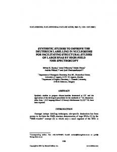
Before illustrating Definition 2, let us introduce some terminology that will be used throughout this article. Definition 3. An arc (i, j) of the associated digraph G of a tree constraint is an S-arc (sure) if dom(VER[i].F) = {j}, otherwise (i, j) is an M-arc (maybe). A vertex i is an S-succ if all its out-going arcs are S-arcs, otherwise i is an M-succ. Similarly, a vertex i is an S-pred if all its incoming arcs are S-arcs, otherwise i is an M-pred. Definition 4. Given a tree(NTREE, NPROP, VER) constraint and its associated digraph G = (V, E), the fixed-father digraph Gtrue = (V, Etrue ) is defined by Etrue = {(i, j) | i 6= j ∧ (i, j) is an S-arc of G}. Example 1. Consider the constraint tree(NTREE, NPROP, VER), where dom(NTREE) = {1, 2, 3, 4} = dom(NPROP), and the attributes of the vertices are as given in Part (a) of Table 1. The digraph G is depicted in Figure 1(a). In Figure 1(b) and 1(c), precedence constraints are depicted in dashed arcs, while in 1(c) incomparability constraints are in bidirectional dotted arcs. Observe that the degree constraints have no impact on the number of solutions here, as the largest observed in-degree in G does not exceed the maximum value of any in-degree variable. Without considering the precedence, incomparability, and degree constraints, this tree constraint has 220 solutions. When considering only the precedence and degree constraints, the tree constraint has two solutions, depicted in Figures 1(b) and 1(c), with NTREE = 1 = NPROP and NTREE = 2∧NPROP = 1, 4

An elementary path between two vertices i and j of a digraph G, denoted by Phi,ji , is a path from i to j such that all vertices of Phi,ji are distinct.

3

4

5

3

6

2

7

1

8

4

5

3

6

2

7

5

3

6

2

7

8

1

1

(a)

8

4

(b)

(c)

Fig. 1. Figure 1(a) the associated digraph G of the tree constraint given in Example 1. Figure 1(b)-1(c) the two only solutions according to the degree and precedence constraints, the latter being depicted by dashed arcs, going from i to j for each j ∈ [1, n] and each i ∈ VER[j].P. Figure 1(c) the only solution according to the degree, precedence, and incomparability constraints, the latter being depicted by bidirectional dotted arcs, connecting i and j for each i ∈ [1, n] and each j ∈ VER[i].I. Note that within solution 1(b) the vertices 7 and 8 are comparable. i VER[i].L 1 2 3 4 5 6 7 8

1 2 3 4 5 6 7 8

Part (a) Part (b) Part (c) VER[i].F VER[i].P VER[i].D VER[i].F VER[i].D VER[i].F VER[i].I VER[i].D {2, 3, 7} ∅ [0, 4] {2} {0} {2} ∅ {0} {1, 3} {1} [0, 4] {3} {1} {3} ∅ {1} {2, 4, 6} {2} [0, 4] {4} {1} {4} ∅ {1} {4, 5} {1} [0, 4] {5} {1} {5} ∅ {1} {4, 5, 6} {1} [0, 4] {6} {1} {6} {8} {1} {7, 8} ∅ [0, 4] {7} {2} {7} ∅ {1} {6, 7} {1, 5} [0, 4] {7} {1} {7} {8} {1} {6, 8} ∅ [0, 4] {6} {0} {8} ∅ {0}

Table 1. Part (a) provides the domains of the father and degree variables depicted by Figure 1(a), as well as the set of precedence constraints. Part (b) gives a solution for the instance depicted by Figure 1(a). Part (c) provides a solution for the instance depicted by Figure 1(a) enriched by the set of incomparability constraints.

respectively. Finally, when also considering the incomparability constraints, the tree constraint has a single solution, given in Figure 1(c). Note that, since in Figure 1(a) no father variables are fixed, all arcs are M-arcs and all vertices are M-succs and M-preds. As a consequence, Gtrue does not contain any arcs. The rest of this article is organised as follows. First, temporarily ignoring the incomparability, degree, and number-of-proper-trees constraints, Section 2 provides necessary conditions for partitioning the associated digraph G of a tree constraint into trees according to a potential number of trees and a set of precedence constraints only. Since achieving arc-consistency for even this constraint is NP-hard, some pruning rules are derived from relaxations of these necessary conditions. Next, Section 3 completes those results by also considering the incomparability constraints. New necessary conditions are added to ensure that there exists at least one tree partitioning of G according to the 4

precedence and incomparability constraints. Moreover, some pruning rules are derived to enhance the pruning proposed in the previous section. Then, Section 4 shows how to model the degree constraints by adapting the flow model of the global cardinality constraint [18] in order to ignore self-loops.5 Next, the number-of-proper-trees constraint is considered in Section 5. To summarise the theoretical results so far, Section 6 provides a synthetic overview of all propositions of the different aspects of the tree constraint. It shows that many interactions between the tree partitioning, precedence, incomparability, and number-of-proper-trees constraints have been taken into account to improve the filtering. Section 7 then presents our experimental results with the extended tree constraint, including on the problems of constructing a supertree of given phylogenetic species trees and an ordered simple path with mandatory vertices. Finally, Section 8 reviews related work, discusses future work and concludes.

2 Combining the Tree Partitioning and Precedence Constraints We show how to extend the work on the original tree constraint [5] in order to take into account precedence constraints. In Section 2.1, we provide a normal form for a set of precedence constraints and indicate how it can be dynamically updated whenever a new father variable becomes fixed. Then, in Section 2.2, we argue that this normal form can also be updated in the presence of information derived from the associated digraph G of the tree constraint. Next, in Section 2.3, we show how to exploit this normal form in order to get a tighter upper bound on the number NTREE of trees. In Section 2.4, we identify necessary feasibility conditions from the precedence constraints. Finally, in Section 2.5, we derive filtering rules from these necessary conditions. 2.1 Normalising a Set of Precedence Constraints We first show how to handle the precedence constraints provided by the P attributes of the VER collection, and this independently of the tree partitioning constraint. Observe that the set of precedence constraints increases as father variables get fixed: the assignment VER[i].F = j adds a new precedence constraint, namely i ∈ VER[j].P. Towards this, we maintain a normal form of the precedence digraph obtained from all the precedence constraints. Definition 5. The precedence digraph Gp = (V, Ep ) of a tree(NTREE, NPROP, VER) constraint with associated digraph G = (V, E) has as arc set Ep the transitive reduction of {(i, j) | i ∈ VER[j].P}. An arc (i, j) ∈ Ep is called a precedence arc, or P-arc for short. We can derive a trivial necessary condition for the feasibility of a set of precedence constraints according to a tree constraint: Proposition 1. If a tree constraint is feasible, then there do not exist any circuits in the precedence digraph. Proof. Trivially derived from the definition of a precedence. 5

Ignoring the fact that the i-th father variable VER[i].F is eventually assigned value i.

5

t u

Algorithm 1 Adding an arc (i, j) to Gp 1. Checking feasibility: Perform a first depth-first search (DFS) from vertex j, using the successor links of Gp , and mark by 1 all the reached vertices and j. If i is reached, then generate a failure, since a circuit was detected. 2. Checking that (i, j) is not a transitive arc: Perform a second DFS from i to search for j. If j is reached then exit, as the arc (i, j) is transitive and Gp remains unchanged (i.e., (i, j) is not added to Gp ). During this second DFS, we skip the vertices reached in Step 1, since Gp does not contain any circuits. 3. Removing transitive arcs: Perform a third DFS from i, using the predecessor links of Gp , and mark by 2 all the reached vertices as well as i. Remove from Gp all arcs (k, l) where k is 2-marked and l is 1-marked. 4. Updating Gp : Add the arc (i, j) to Gp .

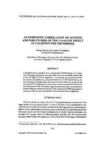
The precedence digraph of a feasible tree constraint is thus a Hasse digraph, that is an acyclic digraph without any transitive arcs [1]. When a tree constraint is posted, the precedence digraph Gp = (V, Ep ) is created, using the algorithm given by [14], with a time complexity of O(n · |Ep |). Then, each time a father variable VER[i].F is fixed to some j (with j 6= i), for instance during search, we add the arc (i, j) to G p by using Algorithm 1, which has a worst-case complexity of O(n + |Ep |) time. Example 2. Consider the tree constraint given by Figure 2(a) and assume that the father variable for vertex 3 is instantiated to vertex 6. Figure 2(b) depicts the state of G and G p after normalisation: the transitive arc (3, 5) was removed from Gp when the arc (3, 6), in bold, was added.

2.2 Deriving Precedence Constraints from G We saw in the previous sub-section that each time some father variable VER[i].F is fixed to some j (that is, each time some (i, j) becomes an S-arc), a new precedence constraint is created and added to Gp . However, there also exist some precedence constraints in Gp that can never be directly satisfied, because there exist arcs (u, v) in G p that are not in G. We thus introduce some updating rules (Propositions 2 to 5 below) for the precedence digraph Gp that add new precedence constraints and replace some precedence constraints that can never be directly satisfied. Let us first show the intuition of these updates on an example. Example 3. Consider again the tree constraint given by Figure 2(b). Then, Figure 2(c) depicts the precedence digraph Gp enriched by new precedence constraints: 6

4

5

4

5

4

5

4

5

4

5

4

5

3

6

3

6

3

6

3

6

3

6

3

6

2

7

2

7

2

7

2

7

2

7

2

7

1

1 G

1 Gp

(a)

1

1 G

Gp

(b)

1 G

Gp

(c)

Fig. 2. 2(a) The digraphs G and Gp of a tree constraint before instantiation of the father variable for vertex 3 to vertex 6. 2(b) The digraphs G and Gp after the choice of the arc (3, 6) and normalisation, where (3, 6) is a new precedence (bold dashed arc). 2(c) The digraph Gp after adding and replacing precedence constraints, where the new precedences are the bold dashed arcs.

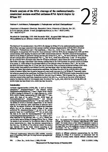
– From Gp , the vertex 1 precedes 6. Moreover, observe that if 2 is removed from G then there are no more paths from 1 to 6 in G. As a consequence, the vertex 1 must precede 2 and (1, 6) becomes a transitive arc of Gp . – As 3 has only successor 6 in G, the precedence (3, 4) cannot be directly satisfied. As a consequence, the precedence (3, 4) is replaced by (6, 4). – Since, within G, all paths from 7 to a vertex having a self-loop contain the vertex 2, the vertex 7 precedes 2. The first two propositions below consider a precedence constraint (j, i) such that i∈ / dom(VER[j].F) and either all predecessors of i in G are already known (i.e., vertex i is an S-pred), or the successor of j is already fixed. In this context, one can try to replace the precedence (j, i). We first need to introduce a terminology and notation derived from [4] for specifying the descendants and ascendants of a given digraph G. Definition 6. Let u and v be two, not necessarily distinct, vertices of a digraph G = (V, E). We say that v is a descendant of u in G (and u is an ascendant of v in G), which is denoted by u C∗G v, if there exists a path from u to v in G. The set of descendants of u u in G is denoted by DG = {v ∈ V | u C∗G v}, and the set of ascendants of v in G is v denoted by AG = {u ∈ V | u C∗G v}. At any given stage, consider for a vertex i the set AiGtrue of its mandatory ancestors in G (i.e., the vertices k such that there is a path from k to i in Gtrue ). Now, consider the restriction of AiGtrue to the vertices reachable from j in G (i.e., AiGtrue ∩ DGj ). Since j has to precede i, there must be a path, in G, from j to one of the vertices of A iGtrue ∩ DGj . As a consequence, we get the following propositions, illustrated by Figure 3(a) and Figure 3(b). Proposition 2. A precedence (j, i) ∈ Ep is replaced by a precedence (j, k) such that k is the first common descendant of the vertices of AiGtrue ∩ DGj . 7

k

i

j

j

AiG true

succ DG i p

i

DGi

sccj

j

p

true

scc

k

i

AiG

true

∩ DGi

(a) Proposition 2

j

scci

i

(b) Proposition 3

(c) Proposition 4

(d) Proposition 5

Fig. 3. Plain arcs represent arcs of G, while dashed arcs represent arcs of Gp . Dashed and bold arcs represent new precedences found by the propositions while barred arcs represent old precedence constraints which are removed. Within graph 3(d), scc represents the original strongly connected component containing the vertices i, j, and p, while scci and sccj represent the two strongly connected components obtained after removing p.

Proposition 3. A precedence (j, i) ∈ Ep is replaced by a precedence (k, i) such that k is the sink of Gtrue contained in DGj true . The following two propositions characterise conditions on G and G p from which new arcs can be added to Gp (see Figures 3(c) and 3(d)). Proposition 4. For each pair of vertices i, j such that j is the first common descendant in Gp of the possible successors of i in G, the arc (i, j) can be added to G p . Proof. Consider the set S of possible successors of a vertex i of G. If there exists a first common descendant j in Gp for the vertices of S, then for every k ∈ S there exists a path from k to j in any solution to the tree constraint. As a consequence, there also exists a path from i to j and the precedence (i, j) can be added to G p . t u Before introducing the next proposition, we need to present the notion of strong articulation point. Definition 7. A strong articulation point of a strongly connected digraph G is a vertex such that, if we remove it, G is broken into at least two strongly connected components. Proposition 5. Given the associated digraph G = (V, E) and the precedence digraph Gp = (V, Ep ) of a tree(NTREE, NPROP, VER) constraint, consider an arc (i, j) ∈ E p and a strong articulation point p of G. If there does not exist a path from i to j in G \ {p}, then the two arcs (i, p) and (p, j) can be added to Gp . Proof. If there exists an arc (i, j) in Ep , then in any solution there exists a path from i to j. Moreover, if the withdrawal of a strong articulation point p implies that i cannot reach j, then there exists a path from i to p and a path from p to j, hence (i, p) and (p, j) are mandatory precedence arcs. t u 8

2.3 Upper Bound on the Number of Trees According to Precedence Constraints We now provide an upper bound on the number of trees that partition the associated digraph G of a tree constraint, according to the precedence digraph G p . We first introduce the notion of potential roots of those trees, namely the vertices with a self-loop in G. Definition 8. A potential root r is a vertex such that r ∈ VER[r].F. A first upper bound, given in [5] and denoted by MAXTREE, is the number of potential roots of G. Since this bound does not consider the precedence constraints, we now provide a tighter bound that considers Gp as well. The idea is to count among the connected components of Gp those that are necessarily connected to another one. For this purpose, a {0, 1}-value is associated to each connected component C i of Gp , depending on whether there is a vertex in Ci whose potential father vertices are all outside Ci . Definition 9. For each connected component Ci of the precedence digraph Gp of a tree constraint, let: ( 1 if ∃u ∈ Ci : ∀v ∈ dom(VER[u].F) : v ∈ / Ci out i = 0 otherwise Proposition 6. Given a tree(NTREE, NPROP, VER) constraint and its precedence digraph Gp , consisting of k connected components, an upper bound on NTREE is: MAXTREEGp = k −

k X

out i

i=1

Proof. From Definition 9.

t u

Proposition 7. MAXTREEGp is tighter than MAXTREE. Proof. Let p = MAXTREE be the number of potential roots of G. We know that: k−p≤

k X

out i ≤ k

i=1

Hence: 0≤k−

k X

out i ≤ p

i=1

Thus, we showed that 0 ≤ MAXTREEGp ≤ MAXTREE.

t u

2.4 Feasibility of a tree Constraint According to the Precedence Constraints We now give necessary conditions for the feasibility of a tree constraint that consider the interaction between the associated digraph G and the precedence digraph G p . We first recall the necessary and sufficient feasibility conditions (Proposition 8) for the 9

original tree constraint [5], which still apply in our context but only as necessary conditions. Since these conditions ignore precedences, we then introduce new necessary conditions (in Proposition 9) for the extended tree constraint and show that their evaluation is NP-complete (Proposition 10). Finally, we derive from Proposition 9 a set of necessary conditions (Propositions 11 and 12) that can be evaluated in polynomial time. Before recalling in Proposition 8 the necessary feasibility conditions [5] obtained for the original tree constraint, we need to introduce some concepts. Definition 10. A strongly connected component of the associated digraph G of a tree constraint that contains at least one potential root is called a rooted component. A strongly connected component of G that has no out-going arcs is called a sink component. Proposition 8 ([5]). There is a solution to a tree(NTREE, VER) constraint iff the following conditions hold: 1. All the sink components of the associated digraph G are rooted components. 2. dom(NTREE) ∩ [MINTREE, MAXTREE] 6= ∅, where MINTREE is the number of sink components in G and MAXTREE is the number of potential roots in G. We now provide general necessary conditions (Proposition 9) for the extended tree constraint that consider the precedence and tree partitioning constraints. We first need to introduce the notion of compatibility of an arc of G with Gp . Definition 11. An arc (u, v), with u 6= v, of G is compatible with Gp if there does not exist an elementary path from v to u in Gp and there does not exist a path of length > 1 from u to v in Gp . The intuition of the next proposition is that, for each vertex u of the associated digraph G of a tree constraint, there should exist an elementary path, from u to a potential root, in G that contains all the descendants of u in the precedence digraph G p , such that each arc of this elementary path is compatible with Gp . Proposition 9. If a tree constraint is feasible, then, for each vertex u of the associated digraph G, there exists an elementary path Phu,ri in G, where r is a potential root, such that: 1. For each vertex v ∈ Phu,ri , the set DGv p is included in the vertices of Phv,ri . 2. Each arc (v, w) of Phu,ri is compatible with the precedence digraph Gp . Proposition 10. Checking Proposition 9 is NP-complete. Proof. Figure 4 shows a configuration of constraints where checking Proposition 9 is equivalent to searching for a Hamiltonian path in G. Since the precedence digraph G p consists of a single connected component with a single source and four sinks, by definition of tree, all sinks have to be located on an elementary path starting from the source. Thus, for this configuration, checking Proposition 9 may be reduced to the HAM-PATH problem [12, p. 199], which is an NP-complete problem. t u 10

3

3 1

2

5

4

2

5 1

4

(a)

(b)

Fig. 4. 4(a) The associated digraph G. 4(b) The precedence digraph Gp . The two only solutions are the Hamiltonian paths h1, 3, 4, 2, 5i and h1, 4, 3, 2, 5i.

We now present polynomial-time necessary conditions involving precedences and show that they are derived from the general necessary conditions of Proposition 9. Beyond checking whether each arc of a ground instance of a tree constraint is compatible with the precedence digraph, the following proposition ensures that all the precedence constraints will be effectively represented in a ground instance of a tree constraint. It is derived from a relaxation of Condition 1 of Proposition 9. Proposition 11. If a tree constraint is feasible, then, for each vertex u of the associated digraph G, we have DGup ⊆ DGu , where Gp is the precedence digraph. Proof. Assume that there exists a vertex w ∈ DGup such that w ∈ / DGu . Then, for each vertex v ∈ DGwp , the precedence constraint (v, w) cannot be respected in G. t u The next proposition, derived from Proposition 9, shows how to check whether there exists a feasible potential root in each sink component of G. Proposition 12. If a tree constraint is feasible, then, in each sink component of the associated digraph G, there exists a potential root r that is a sink in the precedence digraph Gp . Proof. The potential root r mentioned in Proposition 9 has to be a sink in G p , otherwise t u Condition 1 of Proposition 9, namely DGup ⊆ Phv,ri , cannot hold. The overall time complexity for checking the feasibility of an extended tree constraint mentioning precedences is O(n · m), since: – Proposition 8 (with MAXTREE replaced by MAXTREEGp ) can be checked in O(n+m) time, as shown in [5]. – Proposition 11 can be checked by the lines 2-8 of Algorithm 2 in O(n · m) time. – Proposition 12 can be checked by the lines 9-10 of Algorithm 2 in O(n · m) time.

2.5 Filtering Related to the Precedence Constraints In the previous sub-section, Proposition 9 was used to derive necessary conditions that can be evaluated in polynomial time. We now show how to further exploit Proposition 9 for pruning the arcs of G according to the precedence constraints. 11

Algorithm 2 Checking feasibility according to Propositions 11 – 12 1. For each sink component Si of G do si ← false; 2. For each vertex u of G do 3. Mark the descendants of u in Gp with a first DFS; 4. Make a second DFS from u in G in the following way: 5. For each arc (v, w) encountered do 6. If vertex w is a descendant of vertex u in Gp then 7. w is marked as reached; // Proposition 11 8. If not all the descendants of u in Gp have been reached by this second DFS then fail; 9. If u is a potential root contained in a sink component Si and u is a sink in Gp then si ← true; // Proposition 12 10. If there exists a sink component Si with si = false then fail;

Proposition 13. For each pair of vertices u, v ∈ V such that (u, v) is not compatible with the precedence digraph Gp , the arc (u, v) is infeasible. Proposition 14. All the arcs (u, v) of G, such that DGup * DGv , are infeasible. Proof. Let us suppose that there exists u0 ∈ DGup , such that u0 ∈ / DGv , then the prece0 dence constraint (u, u ) is violated if the arc (u, v) is enforced in G, thus (u, v) is infeasible. t u Proposition 15. For each potential root r of V that is not a sink in Gp , the arc (r, r) is infeasible. Similarly to the definition of compatible arc of G with Gp (see Definition 11), we now introduce the definition of compatible arc of the reduced digraph of G with G p . The reduced digraph Gr is derived from G in the following way: to each strongly connected component of G we associate a vertex of Gr ; to each arc of G that connects different strongly connected components corresponds an arc in Gr (multiple arcs from a given strongly connected component to another strongly connected component are merged). Definition 12. A transitive arc (ur , vr ) of Gr is compatible with Gp if there does not exist any wr belonging to an elementary path Phur ,vr i (with wr ∈ / {ur , vr }), such that there exist u ∈ ur and w ∈ DGup (with w ∈ wr ). Proposition 16. For each pair of vertices ur , vr of Gr such that the arc (ur , vr ) is not compatible with the precedence digraph Gp , all the arcs (u, v) in G, such that u ∈ ur and v ∈ vr , are infeasible. Proof. Since w ∈ DGup , there must exist a path from u to w in G (see Figure 5). If an arc (u0 , v 0 ) (u0 ∈ ur and v 0 ∈ vr ) is enforced in G then there does not exist anymore paths from u to w since w cannot be reached anymore from v 0 (i.e., Gr does not contain any circuit). t u 12

vr

wr

w v ur

u

(a)

(b)

Fig. 5. 5(a) The set of descendants of u in Gp . 5(b) Gr such that each vertex (subscripted by r) represents a strongly connected component of Gp .

Algorithm 3 removes the infeasible arcs detected by Propositions 13, 14, 15, and 16 in O(n · m) time. Indeed, the time complexity is dominated by the complexity of computing the transitive closures (lines 1-2) inherent to the precedence digraph G p and the digraph G.

3 Taking into Account the Incomparability Constraints We now show how to extend the results of Section 2 in order to take into account the incomparability constraints. In Section 3.1, we characterise hidden incomparability constraints, in order to improve the detection of infeasible arcs in G. Finally, in Section 3.3, we derive filtering rules from these necessary conditions. 3.1 Deriving Incomparability Constraints from Gp Section 2 has shown that new precedence constraints can be added as the father variables get progressively fixed. Similarly, the next proposition shows that the precedence digraph Gp implicitly contains more and more incomparability constraints as new precedences are dynamically added. As a consequence, detecting the structural incomparability constraints hidden in Gp leads to improving the filtering dedicated to incomparability constraints. Proposition 17. For each pair of incomparable vertices u, v, all the ancestors of u in Gp are incomparable with all the ancestors of v in Gp (see Figure 6). Proof. First, suppose that a path from wu ∈ AuGp to wv ∈ AvGp is enforced in G. Then in all solutions there must exist a path from wu to u as well as a path from wv to v (in order to respect precedence constraints). But such a path starts from w u and reaches wv , u, and v, which is impossible because of the precedence constraints (w u , u) and (wv , v). So there does not exist any path from wu to wv in G. Similarly, there does not exist any path from wv to wu in G. t u 13

Algorithm 3 Filtering according to Propositions 13-16 1. Compute the transitive closure T (Gp ) of Gp ; 2. Compute the transitive closure T (G) of G; // Proposition 13 3. For each arc (u, v) ∈ G such that (u, v) ∈ T (Gp ) and (u, v) ∈ / Gp do 4. Remove (u, v) from G; 5. For each arc (u, v) ∈ G such that (v, u) ∈ T (Gp ) do 6. Remove (u, v) from G; // Proposition 14 7. For each arc (u, v) ∈ G such that ∃(u, w) ∈ T (Gp ) and (v, w) ∈ / T (G) do 8. Remove (u, v) from G; // Proposition 15 9. For each vertex u of G do 10. If u is a potential root in a sink component of G and u is not a sink in Gp then 11. Remove the self-loop (u, u) from G; // Proposition 16 12. Given ir a vertex of Gr , compute Sourceir the set of source vertices of Gp such that ir contains at least one vertex which is a descendant of a source vertex of Gp ; 13. For each ir of Gr containing at least one source of Gp do 14. Perform a DFS, DFSiGrr in Gr , starting from ir and exploring first the vertices jr such that Source ir ∩ Sourcejr 6= ∅; 15. For each arc (ur , vr ) of Gr which is transitive in DFSiGrr do 16. If there exists wr between ur and vr in DFSiGrr and Sourcewr ∩ Sourceir 6= ∅ then Remove (ur , vr ) from Gr ;

Let us notice that a side effect of the previous proposition is that incomparable vertices do not have a common ancestor in Gp otherwise the constraint is infeasible. 3.2 Feasibility of a tree Constraint According to Incomparability Constraints We now give two necessary conditions for the feasibility of an extended tree constraint that consider the interaction between the set of incomparability constraints and the associated digraph G (Figure 7(a)) as well as the precedence digraph G p (Figure 7(b)). Proposition 18. If a tree constraint is feasible then, for each connected component C i of Gtrue rooted in ri , there exists at least one successor s of ri in G such that, for every vertex u ∈ Ci , there does not exist a vertex v ∈ DGs true that is incomparable with u. Proof. If there exists an incomparability constraint between a vertex u ∈ C i and a vertex v of DGs true , then the arc (ri , s) cannot be added to Gtrue . t u Proposition 19. If a tree constraint is feasible then, for every incomparability constraint between two vertices u and v of G, we must have neither u C∗Gp v nor v C∗Gp u. 14

u

v

wu

wv

AuGp

AvGp

Fig. 6. If u and v are two incomparable vertices of G (dashed edge (u, v)), then all the ancestors of u in Gp become incomparable with all the ancestors of v in Gp (dashed edge (wu , wv )). v

DGs

DGup

true

s

v

ri

u

Ci

u

(a) Propositions 18

(b) Propositions 19

Fig. 7. Two fail cases for Propositions 18 and 19.

Proof. We cannot maintain both a precedence and an incomparability constraint between two vertices of G. t u Algorithm 4 checks the feasibility of the incomparability constraints in O(n · m) time. Indeed, Lines 1-6 (i.e., Proposition 18) are checked in O(n·m) time and Lines 7-9 (i.e., Proposition 19) are checked in O(n2 ) time because DGup and DGv p are incrementally maintained. 3.3 Filtering Related to the Incomparability Constraints Given a tree constraint and one of its incomparability constraints, we now show how to filter the father variables according to the associated digraph G (Figure 8(a)), the precedence digraph Gp (Figure 8(b)), and the number NTREE of trees (when NTREE = 1). Proposition 20. Given a tree constraint and its associated digraph G = (V, E), consider two incomparable vertices u and v that belong to two distinct connected components of the fixed-father digraph Gtrue that have ru and rv as roots. All the arcs (ru , w) ∈ E (resp. (rv , w) ∈ E) such that w C∗Gtrue v (resp. w C∗Gtrue u) are infeasible. 15

Algorithm 4 Checking feasibility according to Propositions 18-19 // Proposition 18 1. For each connected component Ci of Gtrue do 2. incompatible ← 0; 3. Let S be the set of successors in G of the root ri of Ci ; 4. For each vertex s ∈ S do 5. If there exists u ∈ Ci and v ∈ DGs true with v ∈ VER[u].I or u ∈ VER[v].I then incompatible ← incompatible + 1; 6. If |S| = incompatible then fail; // Proposition 19 7. For each vertex u of G do 8. For each v ∈ VER[u].I do 9. If v ∈ DGup ∨ u ∈ DGv p then fail;

ru

rv

wu

DGup

v

v

u u

w

Cu

wv

Cv

AvGp

(b) Proposition 21

(a) Proposition 20

Fig. 8. Illustrations of filtering rules given by Propositions 20 and 21.

Proof. If there exists an arc (ru , w) ∈ E such that w C∗Gtrue v, then ru C∗G v and we infer that u C∗G v, hence an incomparability constraint is violated. The proof is similar for an arc (rv , w) ∈ E. t u Proposition 21. Given a tree constraint, its associated digraph G = (V, E), and its precedence digraph Gp , consider two incomparable vertices u and v. All the arcs (wu , wv ) ∈ E such that u C∗Gp wu and wv C∗Gp v are infeasible. Proof. If there exists an arc (wu , wv ) ∈ E such that u C∗Gp wu (resp. v C∗Gp wu ) and wv C∗Gp v, then u C∗G v and the incomparability constraint involving u and v is violated. t u Proposition 22. Given a tree(1, NPROP, VER) constraint and its associated digraph G = (V, E), all self-loops (v, v) of E such that the vertex v belongs to an incomparability constraint are infeasible. Proof. If a self-loop on v is enforced then v is comparable with all the other vertices of G and then an incomparability constraint is violated. t u Algorithm 5 remove all infeasible arcs of G detected by Propositions 20 to 22. Lines 1–3 filter according to Proposition 20 and lines 4–5 filter according to Propo16

Algorithm 5 Filtering according to Propositions 20-22 // Proposition 20 1. For each connected component Cu of Gtrue with root ru do 2. For each successor w of ru in G do 3. If there exist u ∈ Cu and v ∈ DGwtrue such that u and v are incomparable then Remove (ru , w); // Proposition 21 4. For each vertex u of Gp such that there exists a vertex v incomparable with u do 5. If there exists wu ∈ DGup and wv ∈ AvGp such that (wu , wv ) ∈ G then Remove (wu , wv ); // Proposition 22 6. If NTREE = 1 then 7. For each vertex u such that u belong to an incomparability constraint do Remove (u, u);

sition 21 in O(n · m) time, while lines 6–7 filter according to Proposition 22 in O(n) time.

4 Taking into Account the In-Degree Constraints Constraints on the number of children are quite common in the phylogenetic supertree problem [6] (see Section 7.1) for instance. They also allow the modelling of path partitioning problems without creating any specific path constraint. We now show how to handle such in-degree constraints on the number of children of each vertex. We provide a flow model of this constraint based on the flow model of the global cardinality constraint [18]. To each vertex vi of the associated digraph G of a tree(NTREE, NPROP, VER) constraint, the domain variable VER[i].D, with domain [dimin , dimax ], denotes the number of proper predecessors of vi (i.e., any self-loop on vi is ignored). Observe that the in-degree constraint is very similar to the global cardinality constraint, except that the potential roots have to be handled differently. Figure 9 depicts the modified flow model where an extra value node `, corresponding to potential roots, is added. Formally, the corresponding flow digraph is defined as follows. Definition 13. The flow digraph F = (VF , EF ) of the associated digraph G of a tree(NTREE, NPROP, VER) constraint is defined by: – VF is the union of the following three sets of vertices: • Vlef t = {VER[i].F | i ∈ [1, n]}, each such vertex being labelled by vi . • Vright = {VER[i].L | i ∈ [1, n]}, each such vertex being labelled by i. • {s, t, `}, which are respectively called the source, sink, and loop vertices. – EF is the set of the following capacitated arcs: • There is an arc from the source s to each vertex vi ∈ Vlef t , with a capacity of [1, 1]. 17

l

v1

[0, 1]

1

[1, 1]

[min(NTREE), max(NTREE)] [d1min, d1max]

v2

2

s

[d2min, d2max]

t

[dnmin, dnmax] Vlef t

vn

[0, 1]

n

Vright

[n, n]

Fig. 9. Flow digraph of the associated digraph G. Each left vertex vi represents a father variable, while each right vertex i 6= ` represents a vertex of G. The vertex ` depicts a potential roots (i.e., there is an arc from vi to ` iff i ∈ dom(VER[i].F)).

• There is an arc from the sink t to the source s, with a capacity of [n, n]. • There is an arc from vertex vi ∈ Vlef t to vertex j ∈ Vright , with a capacity of [0, 1], if j ∈ dom(VER[i].F) and j 6= i. • There is an arc from vertex vi ∈ Vlef t to the loop vertex `, with a capacity of [0, 1], if i ∈ dom(VER[i].F). • There is an arc from vertex i ∈ Vright to the sink t, with a capacity of dom(VER[i].D) = [dimin , dimax ]. • There is an arc from the loop vertex ` to the sink t, with a capacity of [min(NTREE), max(NTREE)]. Notice that, for each i ∈ Vright , if i 6= ` then dimin and dimax respectively denote the minimum and maximum values of the in-degree of the vertex v i of G. The number of trees to build is integrated within the flow model as the capacity [min(NTREE), max(NTREE)] on the out-going arc of `. We use the classical flow-based filtering algorithm described in [18] to prune every arc of G that is incompatible with the in-degree constraints.

5 Taking into Account the Number-of-Proper-Trees Constraint In many practical partitioning problems, we do not have to cover all the vertices of the associated digraph G [17]. In this context, the set of vertices that are not covered will be modelled as a set of self-loops. Consequently, we want to distinguish proper trees (i.e., trees involving at least two vertices) from isolated self-loops. Beside the basic inequality NTREE ≥ NPROP, we now show how to propagate according to the variable NPROP corresponding to the number of proper trees. Proposition 23. The minimum number of proper trees, denoted by MINPROP, that can be used to partition G is the number of connected components of G true involving at least two vertices, including a vertex r such that dom(VER[r].F) = {r}. 18

Proposition 24. The maximum number of proper trees, denoted by MAXPROP, that can be used to cover G is the number of potential roots in G minus the number of vertices v such that dom(VER[v].F) = {v} and ∀u 6= v, v ∈ / dom(VER[u].F). The next two propositions filter the arcs of G when one of the two previous bounds on NPROP is reached. Proposition 25. If NPROP = MINPROP, then, for each potential root u that cannot reach a connected component of Gtrue containing at least two vertices including a vertex r such that dom(VER[r].F) = {r}, the self-loop on u is enforced and any other arc (v, u), v 6= u, is removed. Proposition 26. If NPROP = MAXPROP, then for each vertex v such that v ∈ dom(VER[v].F), the self-loop on v is enforced.

6 Synthetic Overview of the tree Constraint Table 2 summarises the theoretical results of this article. It is divided into five horizontal parts. The first part shows that the upper bound on NTREE has been improved over [5] without any overhead. The second part provides upper and lower bounds on the number of proper trees. The third part recalls that evaluating the feasibility of an extended tree constraint is NP-hard and points out some necessary conditions that can be evaluated in polynomial time. The fourth part provides polynomial-time filtering rules derived from the previous necessary conditions. The last part recalls how each instantiation of a father variable leads to updating the precedence digraph Gp as well as the set of incomparability constraints (here denoted by I). For each set of propositions and algorithms an upper bound on the time complexity is provided, where n and m respectively denote the numbers of vertices and arcs in the associated digraph G.

7 Experimental Results We now report on several experiments we have conducted to evaluate the extended tree constraint. First, in Section 7.1, we discuss our experiments on the molecular biology problem of constructing phylogenetic supertrees, both in its pure form and with side constraints. Then, in Section 7.2, we present our results on the routing problem of constructing ordered simple paths with mandatory vertices. Finally, after reporting the performance on random instances of the extended tree constraint in Section 7.3, we make a quantitative and qualitative analysis of its efficiency in Section 7.4. Unless otherwise posted, all experiments were performed with the Choco constraint programming system (which is a Java library) on an Intel Pentium 4 CPU with 3GHz and a 1GB RAM, but with only 32MB allocated to the Java Virtual Machine. 7.1 The Phylogenetic Supertree Problem The objective of phylogeny is to construct the genealogy of the species, called the tree of life (assuming that evolution happens only by mutations, as with recombinations 19

Bounds on NTREE Bounds on NPROP

Feasibility

Direct Filtering

Internal Deductions

Interaction

Effects

G G G & Gp G G G Gp G & Gp G & Gp G&I Gp & I G G G G & Gp G&I Gp & I G & Gp Gp

min(NTREE) max(NTREE) max(NTREE) min(NPROP) max(NPROP)

f ail

G

Gp I

Related Propositions Time Complexity and Algorithms MINTREE, [5], Prop.1 O(n + m) MAXTREE, [5], Prop.2 O(n) MAXTREEGp , Prop. 6 O(n + m) MINPROP, Prop. 23 O(n + m) MAXPROP, Prop. 24 O(n) Prop. 8 (Prop.3 of [5]) O(n + m) Prop. 1 O(n + m) Prop. 9 NP-hard Prop. 11, 12 O(n · m) Prop. 18 O(n · m) Prop. 19 O(n · m) [5], Prop. 5, 6, 7 O(n · m) Section 4, [18] O(n2 · m) Prop. 25, 26 O(n + m) Prop. 13, 14, 15 (12), 16 O(n · m) Prop. 20 (18), 22 O(n · m) Prop. 21 (19) O(n · m) Algo. 1, Prop. 2, 3, 4, 5 O(n2 · m) Prop. 17 O(n · m)

Table 2. Summary of the tree constraint. In the fourth column, “Prop. i (j)” means that Proposition i was derived from Proposition j.

one actually obtains a network), whose leaves represent the contemporary species and whose internal vertices are not necessarily named. An important constraint satisfaction problem in phylogeny is the construction of a supertree [6] that is compatible with several given trees T1 , . . . , Tk (of which any two share at least one species). The given trees and the supertree are not necessarily binary: we speak of polytomy when an internal vertex has more than two subtrees; polytomies can be hard (the mutation was not binary) or soft (information for further structure in the tree is lacking). A first supertree algorithm was given in [2], with an application for database management systems; it takes O(n2 ) time, where n is the number of leaves in the given trees. Many derived algorithms for the supertree problem have emerged from the phylogeny field, for instance [15]. The algorithm in [7] from computational linguistics has supertree construction as a particular case. The first constraint program was proposed in [13], using standard (non-global) constraints. Nowadays, many side constraints to the pure supertree problem are emerging from the demands of biologists. For instance, relative ancestral divergence dates [9] can be used to order speciation events; this gives rise to numerical side constraints of the form mrca(a, b) < mrca(c, d), where mrca(x, y) denotes the rank of the most recent common ancestor of the leaf species x and y, the rank of the root being zero. Addressing this is future work, but trivial for the constraint model of [13]. Another side constraint concerns nested species [19], where the internal vertices of the trees can be named, 20

possibly by names of leaf species of other trees, so that a side constraint emerges for preserving ancestries. Interestingly, our tree constraint is powerful enough to model this side constraint, and it is also simple to adapt the constraint model of [13]. Hence no new algorithms have to be designed for dealing with such side constraints, nor for enumerating all solutions. This is not the case in classical phylogeny research, where new deterministic algorithms have to be designed, and then integrated and made nondeterministic, for each new side constraint. Let us denote the set of vertices of a tree T by N (T ). The supertree problem can be modelled by a tree(1, 1, VER) constraint, such that the associated digraph G is the complete digraph with vertex set V = N (T1 ) ∪ · · · ∪ N (Tk ) and edge set E = {(u, v) | u, v ∈ V}, the precedence digraph Gp = (V, Ep ) is dictated by T1 , . . . , Tk , and the incomparability constraints are generated from the incomparable vertices of each tree T1 , . . . , Tk . All the leaves of T1 , . . . , Tk that are not internal vertices of any tree Ti must remain leaves and thus have an in-degree of zero: VER[i].D = 0. All the other vertices of V have the degree constraint VER[i].D ∈ [1, 2] if a binary supertree is requested, and VER[i].D ∈ [1, n − 1] otherwise, where n = |V|. A smallest-domain heuristic is used to select a father variable at each waking up of the tree constraint, and the value selection heuristic favours, for a selected vertex vi , a father vj such that there exists a minimum-length path from vi to vj or vice-versa in the precedence digraph Gp . Table 3 compares the performance of this constraint program with the one of [13] (which has been improved since then6 ), until the first solution is found or the absence of solutions is established. For the latter model, we have run a re-implementation in OPL 3.7 (which is commonly believed to be 3 to 4 times faster than Choco) on a similar computer, namely an Intel Pentium 4 CPU with 2.53GHz, a 1GB RAM, and a 512 KB cache. There are 17 leaf species in the two spider trees of [19], which were taken from study S1x6x97c14c42c30 in TreeBASE (http://www.treebase.org/); they feature nested species and one of them is not binary, hence there is no binary supertree. There are 23 leaf species in the two cat trees of [19], which were taken from biology journals; one of them is not binary, hence there is no binary supertree. There are 34 leaf species in the two sea-bird trees of [13], which were taken from an ornithology journal; both are binary. As these real-life instances are not small, the numbers of solutions are huge (which is denoted by ≫) on the pure version of the problem (cats and sea birds), but small in the presence of side constraints (spiders). Our model generates symmetric solutions (in the sense that some internal vertices are fathers of only one other vertex, which is also internal, so that their roles can be inverted unless they are named), whereas the one of [13] generates unique solutions modulo all symmetries. On the other hand, our model has only Θ(`) domain variables, where ` is the number of leaf species in the given trees,7 whereas the model of [13] has Θ(`2 ) domain variables. In order to compare the scalability of the two models, six larger instances (given in Appendix A) were randomly generated, such that the two generated trees contain 60 leaves in total and share 6 leaves. For these larger instances, the extended tree constraint always 6 7

Personal communication by Patrick Prosser. In a binary phylogenetic tree, only the leaves have empty subtrees, so if there are ` leaves, then there are 2` − 1 vertices and it does not matter asymptotically whether we count leaves or vertices.

21

Supertree instances degree #trees spiders [19] cats [19] sea birds [13] inst60-10-01 inst60-10-02 inst60-10-03 inst60-10-04 inst60-10-05 inst60-10-06

any binary any binary any binary any binary any binary any binary any binary any binary any binary

13 0 ≫ 0 ≫ ≫ ≫ ≫ ≫ ≫ ≫ ≫ ≫ ≫ ≫ ≫ ≫ ≫

extended tree Gent et al. [13] wake-ups failures time failures time 13 0 72ms 82 80ms 1 0 20ms 3 60ms 22 0 300ms 67 220ms 1 0 20ms 21249 74020ms 10 0 520ms 126 620ms 9 0 486ms 3 700ms 63 5 7738ms 2149 4420ms 46 5 5631ms 1 4620ms 23 0 8919ms 1702 3740ms 22 0 11053ms 2 4500ms 56 0 12972ms 1208 3790ms 39 0 10385ms 0 4340ms 16 0 5253ms 1232 4340ms 16 0 5245ms 0 3840ms 9 0 3801ms 548 3490ms 10 0 6374ms 0 3710ms 32 0 7142ms 1294 3820ms 32 0 7045ms 0 4360ms

Table 3. Results for some phylogenetic supertree construction instances

backtracks rarely (namely at most 5 times), while the model of [13] backtracks significantly more often (namely from 548 to 2149 times) in the non-binary case. However, this robustness of the extended tree constraint on the number of backtracks penalises significantly its run time performance (after adjusting for the difference between Choco and OPL, it is not significantly faster than the model of [13]). The supertree problem becomes a constraint optimisation problem if some of the given trees are inconsistent. The so-called ‘modified min-cut’ objective function [16] preserves a maximum of sub-trees of each given tree that are not inconsistent with the other given trees. Addressing this is future work. 7.2 The Ordered Simple Path Problem with Mandatory Nodes The ordered disjoint path problem (ODP) consists in partitioning a given (di)graph G = (V, E) into k mutually vertex-disjoint paths [12, p.217] subject to precedence constraints between some vertices. We here consider a restriction of this problem, called the ordered simple path problem with mandatory nodes (OSPMN) and described in [17], which consists in finding a simple path containing a set of mandatory vertices in a given order. The OSPMN problem can be modelled by a tree constraint such that the associated digraph G is the digraph to be covered, but enriched by a loop on each vertex, while the set of mandatory vertices is contained in a connected component of the precedence digraph Gp such that each mandatory vertex succeeds the first vertex of the path and 22

extended tree Quesada et al. [17] wake-ups failures time failures time 22 7 0 0.071sec 13 4.45sec 22Full 3 0 0.036sec 0 1.22sec 52b 20 0 1.685sec 100 402sec 52Full 6 0 0.692sec 3 45.03sec 52Order a 16 0 0.892sec 16 57.07sec 52Order b 1 0 0.020sec 41 117sec

OSPMN instances SPMN SPMN SPMN SPMN SPMN SPMN

Table 4. Results for the OSPMN instances in [17]

precedes the final vertex of the path, and if there exist precedence constraints between two mandatory vertices, then an arc is added between them. All the other vertices represent connected components of size 1 in Gp . An ordered-path heuristic is used to select a father variable at each waking up of the tree constraint. This heuristic forces an incremental building of the path by selecting as new variable to instantiate the value chosen at the previous step: when an arc (vi , vj ) is enforced at a given step, then an arc starting from vj is selected at the next step. Table 4 shows that this model based on the extended tree constraint compares favourably, both in time and the number of failures, with the results reported in [17] (which have been improved since then8 ) for an equivalent hardware, until the first solution is found or the absence of solutions is established. Within [17] three constraints (namely domReachability, noCycle, and All Different) are used to model the OSPMN problem, and multiple views of the graph G are explicitely represented as graph variables. 7.3 Random Instances for the Hamiltonian Path Problem Two models for the Hamiltonian path problem can be proposed using the extended tree constraint. First, the Hamiltonian path problem is a tree constraint for which each vertex of the given digraph G has an in-degree of exactly one, excepted the origin vertex of the path which have a in-degree of zero. Second, it is possible to add a set of precedences in the instance such that the origin of the path precedes all the other vertices of G and all these vertices precede the final vertex of the path. For each density9 in [0.10, 1], with a step of 0.05, a total of 100 random connected digraphs G of sizes 25, 50, 75, 100, and 150 were considered. For any size of G among {25, 50, 75, 100, 150}, notice that adding precedences to the instance improves significantly the results on the number of backtracks and does not increase the average time complexity. Moreover, the standard deviation of the number of backtracks when precedences are added is significantly lower than without adding the precedence constraints. Thus, adding dynamically precedence constraints provides a strong robustness on the number of backtracks and the standard deviation. Notice that for the instances of size 8 9

Personal communication by Luis Quesada. The density of a digraph G of size n is nm2 , where m is the number of arcs of G.

23

100

1

50

0,5

0

10

50

5

0

1

(a) Instances of size 25 with precedences time standard deviation backtracks standard deviation average time average backtracks

2

1

1

0

time (sec)

3 # backtracks

time (sec)

2

0.50 density

0.75

2

1

20

2 1.5

10

1

5

15

time (sec)

15

0.5

0 0.50

density

0.75

10

0 0.50

density

0.75

1

20

time standard deviation backtracks standard deviation average time average backtracks

15

10

10

5

5

0

0 0.25

20

(d) Instances of size 50 without precedences

# backtracks

time (sec)

20

30

time standard deviation average backtracks average time backtracks standard deviation

0.25

2.5

time standard deviation backtracks standard deviation average time average backtracks

1

1

(c) Instances of size 50 with precedences 25

density

0.75

0

0. 0.25

0.50

(b) Instances of size 25 without precedences 3

3

0 0.25

# backtracks

0.75

# backtracks

0.50 density

15

100

0

0.25

time standard deviation backtracks standard deviation average time average backtracks

# backtracks

1.5

150

time (ms)

150

time (ms)

2

time standard deviation backtracks standard deviation average time average backtracks

# backtracks

200

0 0.25

1

(e) Instances of size 75 with precedences

0.50

density

0.75

1

(f) Instances of size 75 without precedences

150, the deviation between the case for which precedences are dynamically added and the case without any precedences is poor. Obviously, there exists pathological graphs, such as Tutte’s graph [21],10 for which we still need 179 backtracks to prove that there do not exist any Hamiltonian circuits. 7.4 Quantitative and Qualitative Evaluation Phylogenetic Supertree Problems: the sea-bird phylogenetic instance has a complete associated digraph G of size 66 (i.e., 66 vertices and 662 = 4356 arcs). The precedence digraph Gp is built from the two given trees. The set I of incomparability constraints is computed from the incomparable vertices of the given trees. Table 3 shows that, in the unrestricted case, the tree constraint solves this instance in 10 search vertices, 0 backtracks, and 520ms. 10

Tutte’s graph is a non-Hamiltonian 3-connected cubic graph of size 46.

24

2

40

20

20

10

0

0 0.25

0.5

density

0.75

0 0.25

400

time (sec)

# backtracks

time (sec)

200

0.5

100 0 0.50 density

0.75

density

0.75

1

1

time standard deviation backtracks standard deviation average time average backtracks

300 200

0.5

100 0

0 0.25

0.50

(h) Instances of size 100 without precedences 1

time standard deviation backtracks standard deviation average time average backtracks

300

0

1

(g) Instances of size 100 with precedences 400

30

# backtracks

0.5

time (sec)

4

time standard deviation backtracks standard deviation average time average backtracks

60

1

0 0.25

1

(i) Instances of size 150 with precedences

# backtracks

time standard deviation backtracks standard deviation average time average backtracks

# backtracks

time (sec)

6

0.50

density

0.75

1

(j) Instances of size 150 without precedences

Figure 10 shows that not all parts of the tree constraint are necessary to construct a phylogenetic supertree. Figure 10(k) gives the pruning importance of each part of the tree constraint that is actually used to solve the instance. Note that the precedence, incomparability, and degree (GCC) constraints are sufficient to solve this instance efficiently, i.e., even the tree partitioning constraint does not improve the results. Moreover, Figure 10(l) highlights that the incomparability constraints are a very important aspect of the phylogenetic supertree problem. Indeed, if we inhibit the pruning related to the incomparability constraints (Prop.s 20 to 22), then the run time and the number of backtracks during the search increase vary significantly. Figure 11 shows the dynamic aspects of the precedence and incomparability constraints. Figure 11(a) shows that inhibiting the internal derivations (which dynamically add new precedence and incomparability constraints, Prop.s 2 to 5 and Prop. 17) significantly modifies the pruning importance of each part of the tree constraint: the part of the pruning due to the search increases, while the part due to the incomparability constraints decreases. Moreover, Figure 11(b) illustrates that dynamically adding new precedence constraints significantly improves the run time and the number of backtracks. Note that adding incomparability constraints does not improve the performance, because all the potential pruning is carried out during the initial propagation step. The same pattern is followed by the spider and cat phylogenetic instances. Ordered Simple Path Problem With Mandatory Nodes Problems: the SPMN 52Order a OSPMN instance has an incomplete associated digraph G of size 52 (namely 52 vertices and 216 arcs). The precedence digraph G p is composed of one connected component of size 7, and 45 connected components of a single vertex each, and 25

20

time (sec.)

backtracks 40000 > 60 sec

Prec. Incomp. GCC Search

10

> 39000 btcks

time backtracks

20000

0

0

original

(k) Pruning distribution

prec.

incomp.

gcc

(l) Run time and backtracks when some parts of the tree constraint are inhibited

Fig. 10. Pruning effectiveness on the sea-bird phylogenetic instance 20

Search Incomp. GCC Prec.

backtracks

time (sec.) > 60 sec

40000

> 39000 btcks

10

20000

time backtracks 0

0

original

prec.

incomp.

(a) Pruning distribution without any internal (b) Run time and backtracks when some internal derivations derivations are inhibited

Fig. 11. Effectiveness of the internal derivations on the sea-bird phylogenetic instance

there are no incomparability constraints. Table 4 shows that the tree constraint solves this instance in 16 search vertices, 0 backtracks, and 0.892 seconds. Figure 12 shows that, as for the phylogenetic supertree problem, not all parts of the tree constraint are necessary to construct an OSPMN. Figure 12(a) gives the pruning importance of each part of the tree constraint that is actually used to solve the instance. Note that the precedence, degree (GCC), and number-of-proper-trees constraints are sufficient to solve this instance efficiently, i.e., even the tree partitioning constraint does not improve the results and the incomparability constraints are not used. Figure 12(b) shows that the pruning of the degree and number-of-proper-trees constraints cannot be inhibited, as otherwise the constraint would not build or enforce a path partitioning of G. As a consequence, only the pruning related to the precedence constraints can be inhibited and the figure shows that inhibiting this pruning increases the number of backtracks from 0 to 34, and the run time from 0.892 to 8.60 seconds. Figure 13 shows the dynamics aspect of the precedence and incomparability constraints. Figure 13(a) shows that inhibiting the internal derivations significantly modifies the pruning importance of each part of the tree constraint: the part of the pruning due to the precedence constraints is divided by 6.4, the part of the pruning due to the search increases of a factor 3, and the pruning rules related to the original tree partitioning constraint, which are not used when the internal derivations are applied, now detect infeasible arcs. Moreover, Figure 13(b) illustrates that dynamically adding new precedence constraints significantly improves the number of backtracks, as well as the 26

30

time (sec.)

backtracks

45

25 20

time backtracks

30

15 10

15

5

Prec. GCC Nproper Pruning due to search

(a) Pruning distribution

mandatory

0

0

original

prec.

gcc

nproper

(b) Run time and backtracks when some parts of the tree constraint are inhibited

Fig. 12. Pruning effectiveness on the SPMN 52Order a instance

30

time (sec.)

backtracks

45

25 20 15

time backtracks

30

10

15

5

Prec. Tree Part. GCC Nproper Pruning due to search

mandatory

0

0

original

prec.

gcc

nproper

(a) Pruning distribution without any inter- (b) Run time and backtracks when some internal nal derivations derivations are inhibited

Fig. 13. Effectiveness of the internal derivations on the SPMN 52Order a instance

run time which falls from 7.30 seconds to 0.892 seconds. Note that adding incomparability constraints does not improve the performance, because each new incomparability constraint is already respected in the digraph G. The same pattern is followed by the other considered OSPMN instances.

8 Conclusion The tree and path constraints have been unified within a single global constraint. Moreover, we have shown how to handle in a uniform way a variety of useful side constraints, such as precedence, incomparability, and degree constraints, which occur often in the context of path and tree problems. Our approach outperforms an existing path constraint, but can also handle the phylogenetic supertree problem, for instance. As shown by our qualitative evaluation, the key point of the filtering is to derive dynamically new precedence and incomparability constraints. Our experiments, particularly 27

on dense graphs, point to an important topic for future research: finding efficient filters that avoid triggering heavy algorithms when there is obviously nothing to prune.

References 1. A. V. Aho, M. R. Garey, and J. D. Ullman. The transitive reduction of a directed graph. SIAM Journal of Computing, 1(2), 1972. 2. A. V. Aho, Y. Sagiv, T. Szymanski, and J. D. Ullman. Inferring a tree from lowest common ancestors with an application to the optimization of relational expressions. SIAM Journal of Computing, 10(3):405–421, 1981. 3. E. Althaus, D. Duchier, A. Koller, K. Mehlhorn, J. Niehren, and S. Thiel. An efficient graph algorithm for dominance constraints. Journal of Algorithms, 48(1):194–219, May 2003. Special Issue on SODA’01. 4. R. Backofen, J. Rogers, and K. Vijay-Shanker. A first-order axiomatization of the theory of finite trees. Journal of Logic, Language, and Information, 4(1):5–39, 1995. 5. N. Beldiceanu, P. Flener, and X. Lorca. The tree constraint. In R. Bart´ak and M. Milano, editors, Proceedings of the Second International Conference on Integration of AI and OR Techniques in Constraint Programming for Combinatorial Optimization Problems (CP-AIOR’05), volume 3524 of LNCS, pages 64–78. Springer-Verlag, 2005. 6. O. R. Bininda-Emonds, J. L. Gittleman, and M. A. Steel. The (super)tree of life: Procedures, problems, and prospects. Annual Reviews of Ecological Systems, 33:265–289, 2002. 7. M. Bodirsky and M. Kutz. Pure dominance constraints. In Proceedings of STACS’02, volume 2285 of LNCS, pages 287–298. Springer-Verlag, 2002. Submitted journal version, entitled “Determining the consistency of partial tree descriptions”, available at http: //www.informatik.hu-berlin.de/∼bodirsky/en/publications.php. 8. E. Bourreau. Traitement de contraintes sur les graphes en programmation par contraintes. PhD thesis, University of Paris 13, France, March 1999. In French. 9. D. Bryant, C. Semple, and M. Steel. Supertree methods for ancestral divergence dates and other applications. In O. R. Bininda-Emonds, editor, Phylogenetic Supertrees: Combining Information to Reveal the Tree of Life, volume 3, pages 129–151. Kluwer, 2004. 10. H. Cambazard and E. Bourreau. Conception d’une contrainte globale de chemin. In Proceedings of the Dixi`emes Journ´ees Nationales sur la R´esolution Pratique de Probl`emes NPComplets (JNPC’04), pages 107–120, 2004. In French. 11. A. Cayley. A theorem on trees. Quart. J. Math., 23:376–378, 1889. 12. M. R. Garey and D. S. Johnson. Computers and Intractability: A Guide to the Theory of NP-Completeness. Freeman, New York, 1978. 13. I. P. Gent, P. Prosser, B. M. Smith, and W. Wei. Supertree construction using constraint programming. In F. Rossi, editor, Proceedings of CP’03, volume 2833 of LNCS, pages 837– 841. Springer-Verlag, 2003. 14. A. Goralcikiova and V. Konbek. A reduct and closure algorithm for graphs. In Mathematical Foundations of Computer Science, volume 74, pages 301–307. Springer-Verlag, 1979. 15. M. P. Ng and N. C. Wormald. Reconstruction of rooted trees from subtrees. Discrete Applied Mathematics, 69:19–31, 1996. 16. R. D. Page. Modified mincut supertrees. In Proceedings of WABI’02, volume 2452 of LNCS, pages 537–551. Springer-Verlag, 2002. 17. L. Quesada, P. Van Roy, Y. Deville, and R. Collet. Using dominators for solving constrained path problems. In P. Van Hentenryck, editor, Proceedings of PADL’06, volume 3819 of LNCS, pages 73–87. Springer-Verlag, 2006.

28

18. J.-C. R´egin. Generalized arc consistency for global cardinality constraint. In Proceedings of AAAI’96, pages 209–215, 1996. 19. C. Semple, P. Daniel, W. Hordijk, R. D. Page, and M. Steel. Supertree algorithms for ancestral divergence dates and nested taxa. Bioinformatics, 20:2355–2360, 2004. 20. S. Thiel. Efficient Algorithms for Constraint Propagation and for Processing Tree Descriptions. PhD thesis, Universit¨at des Saarlandes, Saarbr¨ucken, Germany, 2004. 21. W. T. Tutte. On Hamiltonian circuits. J. London Math. Soc., 21:98–101, 1946.

29

Appendix A

Random Instances for the Phylogenetic Problems

A.1 inst60-10-01 first tree : (((59,(58,57)),((55,54),56)),(53,(((51,50),(((48, 47),49),(46,(45,(44,(((42,43),(41,(40,39))),(38,(((37,36), (34,35)),((33,32),(((30,29),31),((27,26),28))))))))))),52)); second tree : ((25,24),((((21,(20,19)),((18,(17,(((15,(((13,((11, ((((8,7),9),10),6)),12)),14),31)),16),(29,30)))),((27,26), 28))),22),23)); A.2 inst60-10-02 first tree : ((58,59),(57,(((55,54),((53,52),(((((48,47),49),50), 51),((45,(((43,(42,41)),((((40,(((((36,35),37),38),39),(34, ((33,(32,31)),(30,29))))),(28,(27,26))),25),24)),44)),46)))), 56))); second tree : (23,(22,((20,(19,(18,(17,(16,(((13,(12,(11,(10,(( ((((7,(6,29)),((27,26),28)),8),9),25),24))))),14),15)))))), 21))); A.3 inst60-10-03 first tree : ((59,(57,58)),((55,(54,((52,(51,((50,(49,((47,46), 48))),(((((43,42),44),45),41),((39,(((37,((35,34),36)),((32, (31,(30,(29,(28,27))))),33)),38)),40))))),53))),56)); second tree : ((26,25),(((24,23),(22,21)),((((18,(17,(((14, 15),16),13))),19),((((9,((((6,32),((((27,28),29),30),31)), 7),8)),10),11),12)),20))); A.4 inst60-10-04 first tree : ((59,58),((((55,54),((53,((((51,50),(49,48)),52), (47,46))),((44,(43,(42,(41,((39,(38,(37,(36,(34,35))))),40) )))),45))),56),57)); second tree : (33,(32,(31,((30,29),((((26,25),27),(24,(((21,(20, (19,((((15,(14,((12,13),(11,(10,((8,(7,(6,(((37,((35,34),36)), 38),39)))),9)))))),16),17),18)))),22),23))),28))))); 30

A.5 inst60-10-05 first tree : ((58,59),((((55,((54,53),((52,51),(((50,49),48), ((((((42,41),43),44),45),46),47))))),56),((40,39),((38,(37, 36)),((34,33),35)))),57)); second tree : (((31,30),32),(29,(((26,((24,(23,(22,((20,(19, (((16,(15,(14,((12,(11,(10,((((7,(6,((37,36),38))),8), ((33,34),35)),9)))),13)))),17),18))),21)))),25)),27),28))); A.6 inst60-10-06 first tree : ((59,58),(((56,(55,((53,52),54))),((50,((49,(48, (47,46))),((44,(43,((42,41),((((((38,37),(36,((34,(33,((31, (30,(29,28))),32))),35))),39),40),27),26)))),45))),51)),57)); second tree : ((25,((23,22),24)),((20,(19,((18,17),((16,15), ((((12,(11,10)),13),14),(((9,8),7),(6,((((30,(29,28)),31), 27),26)))))))),21));

31