Comparing Results of 31 Algorithms from the Black-Box ... - CMAP

Comparing Results of 31 Algorithms from the Black-Box Optimization Benchmarking BBOB-2009 Nikolaus Hansen

Anne Auger

Raymond Ros

INRIA Saclay, TAO team LRI, Bat 490 Univ. Paris-Sud 91405 Orsay Cedex France

INRIA Saclay, TAO team LRI, Bat 490 Univ. Paris-Sud 91405 Orsay Cedex France

INRIA Saclay, TAO team LRI, Bat 490 Univ. Paris-Sud 91405 Orsay Cedex France

Steffen Finck

Petr Pošík

Research Center PPE, Univ. of Applied Science Vorarlberg Hochschulstrasse 1 6850 Dornbirn, Austria

Czech Technical University in Prague, Dept. of Cybernetics Technická 2 166 27 Prague 6, Czech Rep.

ABSTRACT This paper presents results of the BBOB-2009 benchmarking of 31 search algorithms on 24 noiseless functions in a black-box optimization scenario in continuous domain. The runtime of the algorithms, measured in number of function evaluations, is investigated and a connection between a single convergence graph and the runtime distribution is uncovered. Performance is investigated for different dimensions up to 40-D, for different target precision values, and in different subgroups of functions. Searching in larger dimension and multi-modal functions appears to be more difficult. The choice of the best algorithm also depends remarkably on the available budget of function evaluations.

Categories and Subject Descriptors G.1.6 [Numerical Analysis]: Optimization—global optimization, unconstrained optimization; F.2.1 [Analysis of Algorithms and Problem Complexity]: Numerical Algorithms and Problems

General Terms Algorithms, performance

Keywords Benchmarking, black-box optimization

1. INTRODUCTION AND METHODS This paper presents running time results from BBOB2009—the Black-Box Optimization Benchmarking workshop at the Genetic and Evolutionary Computation Conference (GECCO) 2009. 31 real-parameter optimization algorithms

(see Appendix) have been tested in a black-box scenario on 24 noiseless benchmark functions. The experimental procedure is detailed in [16], the functions are presented in [10, 17]. Performance results for each algorithm on each function can be found in the original publications. Tables with results of all algorithms on each single function are available at http://coco.gforge.inria.fr/doku.php?id= bbob-2009-results. In the following, we present summarizing results and results on function groups. The performance measure adopted in this paper is the runtime (RT). For measuring a runtime, a target precision value ∆ft = ftarget − fopt is defined. In a single run, an algorithm can either succeed or fail to reach precision ∆ft . In case of a success, the runtime is the number of function evaluations until ∆ft was reached. In case of a failure we can restart the algorithm. Assuming a positive success probability in a single run (a mild assumption for a stochastic search algorithm) the repeatedly restarted algorithm (that terminates, if ∆ft is reached) has a success probability of one! Its running time is the number function evaluations until ∆ft was reached. In this paper, simulated runtime instances of the virtually restarted algorithm are displayed. We obtain a simulated runtime instance from a set of given trials (from the BBOB-2009 data) of the algorithm on a given function: if not a single trial in the set reached ∆ft , we set RT to infinity; otherwise, we draw trials uniformly at random with replacement until a trial is found that reached the target precision ∆ft . The runtime instance is then computed as the sum of function evaluations from all trials drawn. For the last trial only those function evaluations are taken into account that were executed until ∆ft was reached. The expected value of (the simulated) RT obeys s b eval E(RT(∆ft )) = E(N )+

Permission to make digital or hard copies of all or part of this work for personal or classroom use is granted without fee provided that copies are not made or distributed for profit or commercial advantage and that copies bear this notice and the full citation on the first page. To copy otherwise, to republish, to post on servers or to redistribute to lists, requires prior specific permission and/or a fee. GECCO’10, July 7–11, 2010, Portland, Oregon, USA. Copyright 2010 ACM 978-1-4503-0073-5/10/07 ...$10.00.

1 − pbs b u E(Neval ) , pbs

(1)

s b eval where E(N ) denotes the average number of function evaluations until ∆ft is reached from those trials that reached u b eval ∆ft ; E(N ) denotes the average number of function evaluation in the remaining (the unsuccessful) trials; pbs denotes the fraction of trials that reached ∆ft . In fact, the true expected runtime of the (truly) restarted algorithm obeys the s u b eval b eval same formula [2], where E(N ) and E(N ) are the ex-

Proportion of functions

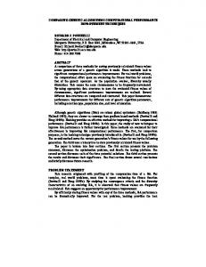
24, 24, 24, 24, 24, 24, 24, 24, 1.0 (24, 24, 24, 24, 24, 24, 24, 24, 24, 24, 24, 24, 24, 24, 24, 24, 24, 24, BIPOP-CMA-ES AMaLGaM IDEA iAMaLGaM IDEA 10-D MA-LS-Chain VNS (Garcia) IPOP-SEP-CMA-ES 0.8 ALPS-GA POEMS Cauchy EDA EDA-PSO (1+1)-CMA-ES DASA 0.6 NELDER (Han) PSO_Bounds G3-PCX NEWUOA NELDER (Doe) PSO (1+1)-ES 0.4 full NEWUOA GLOBAL BFGS Rosenbrock MCS simple GA 0.2 LSfminbnd LSstep DIRECT DE-PSO BayEDAcG Monte Carlo 0.0 0 1 4 5 7 2 3 6 10 10 10 10 10 10 10 10 108 Running length / dimension

Figure 1: Empirical runtime distributions (runtime in number of function evaluations divided by dimension) on all functions with ∆ft ∈ ]100, 10−8 ] in dimension 10. The cross indicates the maximum number of function evaluations. A decline in steepness right after the cross (e.g. for IPOP-SEPCMA-ES) indicates that the maximum number of function evaluations should have been chosen larger. A steep increase right after the cross (e.g. for simple GA) indicates that a restart should have been invoked earlier

pected number of evaluations for successful runs (terminated when ∆ft is reached) and unsuccessful runs respectively, and pbs is the probability of success.

2. RESULTS In general, summarizing results never tell the full story: even if one algorithm solves more functions much faster than others, it does not necessarily perform superior on each and every function. How to read the figures. Each graph in Figure 1 depicts the empirical cumulative distribution of RT of the annotated algorithm on all functions f1 –f24 , in dimension 10. For each function, each ∆ft -value in {101.8 , 101.6 , 101.4 , . . . , 10−8 } is used. We write ∆ft ∈ ]102 , 10−8 ] for this case and use an analogous notation for other cases. Here and in the following 100 instances of RT are generated (using the method described in Section 1) for each function-∆ft -pair. For convenience, we refer to a function-∆ft -pair also as a problem. The x-value in the figure shows a given budget, that is, a given number of function evaluations, divided by dimension. The y-value gives the proportion of problems (function-∆ft pairs), where the ∆ft -value was reached within the given

budget. The graphs are monotonous by definition. Crosses indicate the maximum number of function evaluations observed for the respective algorithm. Results to the right of a cross are only comparable between algorithms with similar maximum number of function evaluations. The limit value to the right indicates the ratio of solved problems. For any given budget (x-value), the proportion of solved problems (y-value) is a useful performance criterion. Even more useful is the horizontal distance between graphs, revealing a difference in runtime for solving the same proportion of problems. The area between two graphs, up to a given y-value, is the average runtime difference (averaged on the log scale), arguably the most useful aggregated performance measure. The best algorithm covers the largest area under its graph. Discussion of Figure 1. Overall, the functions are not easy to solve. Within a budget of 100 × D function evaluations, even the best algorithms can only solve 25% of the problems (20% of the problems have a target precision of ≥ 1). The worst algorithms need 100 times larger a budget to solve 25% of the problems and the diversity of results becomes more pronounced for larger budgets.

∆ft ∈ ]100, 10 ] , 10 t ∈ (24, 24, 24, 24, 24, 24,∆f 24, 24, 24,]10 24, 24, 24, 24, 24, ]24, 24, 24, 24, 24, 24, 24, 24, 24, 24, 24, 24, 24, 2 1.0 (24, 24, 24, 24, 24, 24, 24, 24, 24, 24, 24, 24, 24, 24, 24) = 360 funcs NELDER (Doe) 1.0 iAMaLGaM IDEA VNS (Garcia) AMaLGaM IDEA 2-D 2-D NELDER (Doe) full NEWUOA DIRECT MCS IPOP-SEP-CMA-ES NEWUOA NELDER (Han) ALPS-GA 0.8 0.8 NELDER (Han) VNS (Garcia) BIPOP-CMA-ES iAMaLGaM IDEA PSO GLOBAL (1+1)-CMA-ES ALPS-GA PSO_Bounds IPOP-SEP-CMA-ES (1+1)-CMA-ES AMaLGaM IDEA 0.6 0.6 DASA BFGS MA-LS-Chain Rosenbrock MCS BIPOP-CMA-ES G3-PCX DIRECT POEMS MA-LS-Chain EDA-PSO full NEWUOA EDA-PSO G3-PCX 0.4 0.4 NEWUOA PSO POEMS Rosenbrock PSO_Bounds Cauchy EDA (1+1)-ES Monte Carlo Cauchy EDA GLOBAL simple GA (1+1)-ES 0.2 0.2 BFGS DASA LSstep DE-PSO LSstep simple GA DE-PSO LSfminbnd BayEDAcG Monte Carlo BayEDAcG LSfminbnd 0.0 0 0.0 1 4 5 7 1 4 5 7 2 3 6 8 0 2 3 6 10 10 10 10 10 10 10 10 10 10 10 10 10 10 10 10 10 108 Running length / dimension length dimension (24, 24, 24, 24, 24, 24,Running 24, 24, 24, 24, /24, 24, 24, 24, 24, 24, 24, 24, 24, 24, 24, 24, 24, 24, 24, 24, 24, 2 1.0 (24, 24, 24, 24, 24, 24, 24, 24, 24, 24, 24, 24, 24, 24, 24) = 360 funcs BIPOP-CMA-ES 1.0 BIPOP-CMA-ES AMaLGaM IDEA MA-LS-Chain 10-D 10-D iAMaLGaM IDEA iAMaLGaM IDEA VNS (Garcia) VNS (Garcia) AMaLGaM IDEA MA-LS-Chain ALPS-GA IPOP-SEP-CMA-ES 0.8 0.8 IPOP-SEP-CMA-ES ALPS-GA POEMS POEMS PSO_Bounds Cauchy EDA EDA-PSO EDA-PSO (1+1)-CMA-ES PSO DASA DASA 0.6 NELDER (Han) 0.6 NELDER (Han) NELDER (Doe) G3-PCX (1+1)-CMA-ES NEWUOA PSO_Bounds full NEWUOA simple GA NELDER (Doe) G3-PCX BFGS (1+1)-ES GLOBAL 0.4 0.4 (1+1)-ES NEWUOA Cauchy EDA full NEWUOA GLOBAL PSO MCS Rosenbrock DIRECT MCS simple GA LSfminbnd 0.2 0.2 Rosenbrock LSfminbnd LSstep BFGS LSstep DIRECT DE-PSO DE-PSO BayEDAcG BayEDAcG Monte Carlo Monte Carlo 0.0 0 0.0 1 4 5 7 1 4 5 7 2 3 6 8 0 2 3 6 10 10 10 10 10 10 10 10 10 10 10 10 10 10 10 10 10 108 Running length / dimension length dimension (24, 24, 24, 24, 24, 24,Running 24, 24, 24, 24, /24, 24, 24, 24, 24, 24, 24, 24, 24, 24, 24, 24, 24, 24, 24, 24, 24, 2 1.0 (24, 24, 24, 24, 24, 24, 24, 24, 24, 24, 24, 24, 24, 24, 24) = 360 funcs BIPOP-CMA-ES 1.0 BIPOP-CMA-ES 40-D 40-D AMaLGaM IDEA AMaLGaM IDEA iAMaLGaM IDEA iAMaLGaM IDEA 0.8 IPOP-SEP-CMA-ES0.8 IPOP-SEP-CMA-ES NEWUOA NEWUOA (1+1)-CMA-ES DASA 0.6 0.6 (1+1)-CMA-ES DASA (1+1)-ES (1+1)-ES ALPS-GA BFGS 0.4 0.4 NELDER (Han) BFGS NELDER (Han) ALPS-GA BayEDAcG simple GA 0.2 0.2 BayEDAcG simple GA DE-PSO DE-PSO Monte Carlo Monte Carlo 0.0 0 0.0 0 101 104 105 107 101 104 105 107 10 102 103 106 108 10 102 103 106 108 Running length / dimension Running length / dimension Figure 2: Empirical runtime distributions on all functions with ∆ft ∈ ]100, 10−1 ] (left) and ∆ft ∈ ]10−1 , 10−7 ] (right) in dimension 2, 10, 40 (top to bottom)

For budgets below 500D function evaluations, the best performance achieve NEWUOA, MCS and GLOBAL. For larger budgets, BIPOP-CMA-ES and IPOP-SEP-CMA-ES become superior. The latter sample in each iteration step several solutions from a multivariate Gaussian distribution like all algorithms with a final success ratio ≥ 0.8.

−7

Proportion of functions

Proportion of functions

−1

Proportion of functions

Proportion ofofproblems Proportion functions

Proportion ofofproblems Proportion functions

Proportion ofofproblems Proportion functions

−1

2.1

Search Space Dimensionality

Figure 2 shows the empirical cumulative distribution of RT from all functions f1 –f24 in 2-D, 10-D and 40-D. The right column uses ∆ft -values in ]10−1 , 10−7 ]. The overall problem difficulty strongly increases with increasing dimension. In 2-D, pure Monte Carlo search (the

∆ft = 1

1.0 12 funcs 5-D

0.6 0.4 0.2 0.0 0 101 10 12 funcs 1.0

102

20-D

104 105 103 106 Running length / dimension

107

Proportion of functions

Proportion ofofproblems Proportion functions

0.8 0.6 0.4 0.2 0.0 0 10

∆ft = 10−6

Proportion of functions

Proportion ofofproblems Proportion functions

0.8

12 funcs IPOP-SEP-CMA-ES1.0 BIPOP-CMA-ES 5-D full NEWUOA VNS (Garcia) iAMaLGaM IDEA MA-LS-Chain 0.8 GLOBAL NEWUOA (1+1)-CMA-ES NELDER (Doe) AMaLGaM IDEA Cauchy EDA NELDER (Han) 0.6 G3-PCX ALPS-GA Rosenbrock DIRECT EDA-PSO POEMS 0.4 PSO PSO_Bounds (1+1)-ES DASA BFGS MCS 0.2 simple GA DEPSO LSfminbnd LSstep BayEDAcG Monte Carlo 0.0 0 101 108 10 12 funcs IPOP-SEP-CMA-ES1.0 BIPOP-CMA-ES 20-D (1+1)-CMA-ES iAMaLGaM IDEA AMaLGaM IDEA Cauchy EDA VNS (Garcia) 0.8 MA-LS-Chain NELDER (Doe) NELDER (Han) G3-PCX full NEWUOA 0.6 Rosenbrock NEWUOA GLOBAL ALPS-GA BFGS PSO EDA-PSO PSO_Bounds 0.4 POEMS DASA MCS (1+1)-ES DIRECT 0.2 DEPSO LSfminbnd simple GA LSstep BayEDAcG Monte Carlo 0.0 0 101 108 10

101

102

104 105 103 106 Running length / dimension

107

BIPOP-CMA-ES IPOP-SEP-CMA-ES AMaLGaM IDEA iAMaLGaM IDEA VNS (Garcia) (1+1)-CMA-ES MA-LS-Chain Cauchy EDA BFGS GLOBAL NEWUOA G3-PCX full NEWUOA EDA-PSO (1+1)-ES NELDER (Doe) NELDER (Han) ALPS-GA PSO_Bounds POEMS DASA Rosenbrock LSfminbnd MCS PSO LSstep DEPSO BayEDAcG DIRECT simple GA Monte Carlo 108 IPOP-SEP-CMA-ES iAMaLGaM IDEA AMaLGaM IDEA BIPOP-CMA-ES VNS (Garcia) G3-PCX MA-LS-Chain Cauchy EDA NEWUOA (1+1)-CMA-ES (1+1)-ES BFGS GLOBAL DASA NELDER (Han) full NEWUOA PSO MCS NELDER (Doe) POEMS EDA-PSO Rosenbrock PSO_Bounds ALPS-GA LSfminbnd LSstep BayEDAcG DIRECT DEPSO simple GA Monte Carlo 108

104 105 107 104 105 107 103 106 102 103 106 Running length / dimension Running length / dimension Figure 3: Empirical runtime distributions on 12 unimodal functions f1 , f2 , f5 –f14 with target precision ∆ft = 1 (left) and ∆ft = 10−6 (right) in dimension 5 (above) and 20 (below) 102

worst algorithm) can solve about 40% of the problems (function∆ft -pairs) in about 106 × D function evaluations. In 10-D, the fraction of solved problems becomes invisible for Monte Carlo and half of all algorithms drop below 40%. The spread between the best and the worst algorithms widens remarkably with increasing dimension. • In 2-D, NELDER (Doe) is overall clearly the best algorithm. Only for tiny budgets of less than 20D = 40 function evaluations, it does not solve the most problems. In 3-D, it still performs very well (not shown), while in 5-D other algorithms take over (cp. Fig. 5). • In larger dimension, the picture is more diverse. The best performance depends more significantly on the given budget, as already discussed in Fig. 1. The left column of Fig. 2 shows data with the more easy target precision values ∆ft ∈ ]100, 10−1 ]. The algorithms perform overall better. Nevertheless, more often than not, their individual performance coincides with the one for the more difficult targets. When the ∆ft -values are set to the ∆f -values reached by the best algorithm within D function evaluations, MCS clearly performs best in 20-D, suggesting that MCS has implemented its initial procedures most carefully (not shown).

2.2

Essentially Unimodal Functions

Figure 3 shows results on 12 functions, most of which are unimodal, or they have otherwise an attraction region of the global optimum ≫ 50% (i.e. f8 and f9 ). For target precision 10−6 the performance spread is quite pronounced. The above-mentioned set of well-performing algorithms is complemented by BFGS (5-D), full NEWUOA (target precision 1), Rosenbrock (5-D, target precision 10−6 ), NELDER (Doe) (20-D, target precision 1), and LSfminbnd (20-D). Figure 4 shows results on three single functions: f6 Attractive Sector function, a highly asymmetric function, where the optimum lies at the tip of a cone. 15 algorithms show acceptable performance with a performance loss of mostly less than a factor of hundred (horizontal distance) compared to the best algorithm. f8 Rosenbrock function, a classical test function which has one non-global optimum with an attraction region of smaller than 50%. 15 algorithms show acceptable performance. f10 Ellipsoid function, a globally quadratic, ill-conditioned function (condition number 106 ) which is smoothly locally deformed. 12 algorithms show acceptable performance.

(1, 1, 1, 1, 1, 1, 1, 1, 1, 1, 1, 1, 1, 1, 1, 1, 1, 1, 1, 1, 1, 1, 1, 1, 1, 1, 1, 1, 1, 1, 1, 1, 1, 1, 1, 1, 1, 1, 1, 1, 1, BFGS full NEWUOA 1.0 VNS (Garcia) NEWUOA f8 Rosenbrock MCS (Neum) BIPOP-CMA-ES G3-PCX full NEWUOA GLOBAL NEWUOA BIPOP-CMA-ES IPOP-SEP-CMA-ES0.8 0.8 IPOP-SEP-CMA-ES MA-LS-Chain NELDER (Han) iAMaLGaM IDEA (1+1)-CMA-ES AMaLGaM IDEA G3-PCX POEMS VNS (Garcia) EDA-PSO NELDER (Han) AMaLGaM IDEA 0.6 0.6 (1+1)-ES iAMaLGaM IDEA NELDER (Doe) DASA PSO_Bounds MA-LS-Chain PSO DASA (1+1)-ES BFGS Cauchy EDA ALPS-GA NELDER (Doe) 0.4 PSO 0.4 Rosenbrock Rosenbrock ALPS-GA LSfminbnd EDA-PSO GLOBAL PSO_Bounds (1+1)-CMA-ES LSstep DE-PSO Cauchy EDA LSfminbnd 0.2 0.2 LSstep POEMS simple GA simple GA BayEDAcG DE-PSO BayEDAcG MCS (Neum) DIRECT DIRECT Monte Carlo Monte Carlo 0.0 0 0.0 0 101 104 105 107 101 104 105 107 10 102 103 106 108 10 102 103 106 108 Running length / dimension (3, 3, 3, 3, 3, 3, 3, 3, 3,Running 3, 3, 3, 3,length 3, 3, /3,dimension 3, 3, 3, 3, 3, 3, 3, 3, 3, 3, 3, 3, 3, 3, 3, 3, 3, 3, 3, 3, 3, 3, 3, 3, 3, 1.0 (1, 1, 1, 1, 1, 1, 1, 1, 1, 1) = 10 funcs (1+1)-CMA-ES 1.0 BIPOP-CMA-ES BIPOP-CMA-ES IPOP-SEP-CMA-ES f10 Ellipsoid f &f &f 6 8 10 VNS (Garcia) iAMaLGaM IDEA IPOP-SEP-CMA-ES iAMaLGaM IDEA AMaLGaM IDEA AMaLGaM IDEA VNS (Garcia) 0.8 MA-LS-Chain 0.8 G3-PCX MA-LS-Chain Cauchy EDA NEWUOA G3-PCX BFGS (1+1)-ES NEWUOA (1+1)-CMA-ES GLOBAL Cauchy EDA BFGS 0.6 0.6 (1+1)-ES NELDER (Han) NELDER (Doe) full NEWUOA DASA full NEWUOA NELDER (Han) GLOBAL DASA PSO NELDER (Doe) Rosenbrock ALPS-GA ALPS-GA 0.4 0.4 PSO EDA-PSO PSO_Bounds Monte Carlo PSO_Bounds Rosenbrock POEMS POEMS MCS (Neum) MCS (Neum) LSstep LSfminbnd 0.2 0.2 LSstep LSfminbnd simple GA DE-PSO simple GA EDA-PSO DIRECT DIRECT BayEDAcG DE-PSO BayEDAcG Monte Carlo 0.0 0 0.0 1 4 5 7 1 4 5 7 2 3 6 8 0 2 3 6 10 10 10 10 10 10 10 10 10 10 10 10 10 10 10 10 10 108 Running length / dimension Running length / dimension Figure 4: Empirical runtime distributions on single functions with ∆ft ∈ ]102 , 10−8 ] in dimension 20. For a single trial, the graphs would show a single convergence graph, upside down, with ∆f = 10−10y+2 , where y = −0.1(log10 (∆f ) − 2) ∈ [0, 1] is the annotated y-value. The lower right figure combines the three other figures Proportion of functions Proportion of functions

Proportion ofofproblems Proportion functions

Proportion ofofproblems Proportion functions

1.0 (1, 1, 1, 1, 1, 1, 1, 1, 1, 1) = 10 funcs f6 Attractive Sector

The lower right subfigure combines the convergence data from the three functions. The first nine algorithms listed top (down to BFGS) stay within a performance loss factor of ten (horizontal distance) to the best algorithm up to a y-value of 0.8.

2.3 Multimodal Functions Figure 5 shows running times on the 12 multimodal functions in dimension 5 and 20 (right column) compared to the unimodal functions (left column). The multimodal functions pose a considerably stronger challenge also with a stronger decline with increasing dimension. On multimodal functions in 20-D with larger budgets, BIPOP-CMA-ES clearly outperforms all algorithms but IPOPSEP-CMA-ES, which becomes incomparable for budgets ≫ 104 D. AMaLGaM IDEA outperforms the remaining algorithms for budgets larger than 104 D.

2.4 Function Subgroups Figure 6 shows results for six subgroups of functions. The following algorithms perform particularly well up to their individual maximum number of function evaluations, forming more than 10% of the left envelope of the set of graphs: on separable functions NEWUOA, LSfminbnd and LSstep; on

moderate functions NEWUOA and IPOP-SEP-CMA-ES; on ill-conditioned functions GLOBAL, iAMaLGaM and BIPOPCMA-ES; on the multi-modal structured functions IPOPSEP-CMA-ES and BIPOP-CMA-ES; on the multimodal weakly structured functions GLOBAL and BIPOP-CMA-ES; on nonsmooth functions iAMaLGaM and BIPOP-CMA-ES. The IDEA and *POP*-CMA variants show a quite similar performance characteristics over the subgroups.

3.

CONCLUSIONS

We draw some summarizing conclusions on the BBOB2009 data set. Benchmarks. The benchmark function testbed is comparatively difficult. In dimension 20, within 105 D function evaluations, the best algorithm can solve about 75% of the functions up to a precision of 10−6 , the median algorithm solves about 30%. For the multimodal functions the rate is about 50% (median below 20%). Empirical run time distributions (cf. Fig. 4). A single convergence graph—plotting the best achieved f -value against time—can be interpreted, when plotted upside down, as a cumulative runtime distribution for the set of all f -

values. Exploiting this interpretation, convergence data from several trials can be combined into a single graph. Even data from various functions can be merged into a single graph. During this integration only the labels of single data points to individual trials and functions are lost. Impact on performance. A strong impact on the function difficulty can be found from dimensionality, multi-modality, and non-smoothness. Also different constraints for the time budget (number of function evaluations) have a great impact on which algorithms perform best. Algorithms. For very low dimension, NELDER (Doe) was superior. For lower budgets NEWUOA, MCS and GLOBAL were the best algorithms. For difficult functions and larger budgets, variants of CMA-ES performed best, followed by the AMaLGaM-IDEA variants. The results can provide a clear guideline for the choice of an algorithm or of an ensemble of algorithms in an appropriate way to solve an unknown black-box optimization problem.

4. REFERENCES [1] A. Auger. Benchmarking the (1+1) evolution strategy with one-fifth success rule on the BBOB-2009 function testbed. In Rothlauf (2009, [34]), pages 2447–2452. [2] A. Auger and N. Hansen. Performance evaluation of an advanced local search evolutionary algorithm. In

Proportion of functions Proportion of functions

Proportion ofofproblems Proportion functions

Proportion ofofproblems Proportion functions

12, 12, 12, 12, 12,(12, 12, 12, 12, 12, 12, 12, 12, 12, 12, 12, 12, 12, 12, 12, 12, 12, 12, 12, 12, 12, 12, 12, 12, 12, 12, 12, 12, 12) 1= 1.0 (12, 12, 12, 12, 12, 12, 12, 12, 12, 12, 12, 12, 12, 12, 12, 12, 12, 12, BIPOP-CMA-ES IPOP-SEP-CMA-ES1.0 VNS (Garcia) BIPOP-CMA-ES 5-D unimodal 5-D multimodal AMaLGaM IDEA iAMaLGaM IDEA (1+1)-CMA-ES iAMaLGaM IDEA ALPS-GA AMaLGaM IDEA Cauchy EDA POEMS 0.8 VNS (Garcia) 0.8 MA-LS-Chain IPOP-SEP-CMA-ES MA-LS-Chain NELDER (Doe) PSO NELDER (Han) EDA-PSO NELDER (Doe) G3-PCX simple GA full NEWUOA 0.6 0.6 PSO_Bounds Rosenbrock (1+1)-ES ALPS-GA NELDER (Han) NEWUOA DASA GLOBAL DIRECT BFGS MCS PSO LSstep (1+1)-ES 0.4 0.4 PSO_Bounds (1+1)-CMA-ES POEMS G3-PCX Cauchy EDA EDA-PSO DASA full NEWUOA MCS DEPSO DIRECT GLOBAL 0.2 0.2 DEPSO LSfminbnd simple GA NEWUOA BFGS LSfminbnd LSstep Rosenbrock BayEDAcG BayEDAcG Monte Carlo Monte Carlo 0.0 0 0.0 101 104 105 107 101 104 105 107 10 102 103 106 108 100 102 103 106 108 Running length / dimension length dimension 12, 12, 12, 12, /12, 12, 12, 12, 12, 12, 12, 12, 12, 12, 12, 12, 12, 12, 12, 12, 12, 12, 12, 12, 12, 12,(12, 12, 12, 12, 12, 12, 12,Running 12) 1= 1.0 (12, 12, 12, 12, 12, 12, 12, 12, 12, 12, 12, 12, 12, 12, 12, 12, 12, 12, BIPOP-CMA-ES IPOP-SEP-CMA-ES1.0 AMaLGaM IDEA iAMaLGaM IDEA 20-D unimodal 20-D multimodal BIPOP-CMA-ES iAMaLGaM IDEA IPOP-SEP-CMA-ES AMaLGaM IDEA VNS (Garcia) VNS (Garcia) PSO_Bounds MA-LS-Chain 0.8 0.8 Cauchy EDA MA-LS-Chain DASA G3-PCX ALPS-GA NEWUOA (1+1)-CMA-ES POEMS EDA-PSO BFGS LSstep (1+1)-ES 0.6 0.6 NELDER (Doe) DASA GLOBAL full NEWUOA NEWUOA full NEWUOA NELDER (Han) G3-PCX NELDER (Han) NELDER (Doe) (1+1)-CMA-ES PSO ALPS-GA LSfminbnd 0.4 0.4 (1+1)-ES EDA-PSO GLOBAL Rosenbrock MCS MCS PSO_Bounds simple GA POEMS Rosenbrock PSO LSfminbnd 0.2 0.2 LSstep BFGS Cauchy EDA DEPSO BayEDAcG DIRECT DIRECT DEPSO BayEDAcG simple GA Monte Carlo Monte Carlo 0.0 0 0.0 1 4 5 7 1 4 5 7 2 3 6 8 0 2 3 6 10 10 10 10 10 10 10 10 10 10 10 10 10 10 10 10 10 108 Running length / dimension Running length / dimension Figure 5: Empirical runtime distributions on unimodal (left) and multimodal (right) functions with ∆ft ∈ ]102 , 10−8 ] in dimension 5 and 20. The step observed for LSstep in the lower right is due to the separable functions (see Fig. 6)

[3]

[4] [5]

[6] [7]

[8]

[9]

[10]

Proceedings of the IEEE Congress on Evolutionary Computation (CEC 2005), pages 1777–1784, 2005. A. Auger and N. Hansen. Benchmarking the (1+1)-CMA-ES on the BBOB-2009 function testbed. In Rothlauf (2009, [34]), pages 2459–2466. A. Auger and R. Ros. Benchmarking the pure random search on the BBOB-2009 testbed. In Rothlauf (2009, [34]), pages 2479–2484. P. A. N. Bosman, J. Grahl, and D. Thierens. AMaLGaM IDEAs in noiseless black-box optimization benchmarking. In Rothlauf (2009, [34]), pages 2247–2254. B. Doerr, M. Fouz, M. Schmidt, and M. Wahlstr¨ om. BBOB: Nelder-Mead with resize and halfruns. In Rothlauf (2009, [34]), pages 2239–2246. M. El-Abd and M. S. Kamel. Black-box optimization benchmarking for noiseless function testbed using an EDA and PSO hybrid. In Rothlauf (2009, [34]), pages 2263–2268. M. El-Abd and M. S. Kamel. Black-box optimization benchmarking for noiseless function testbed using particle swarm optimization. In Rothlauf (2009, [34]), pages 2269–2274. M. El-Abd and M. S. Kamel. Black-box optimization benchmarking for noiseless function testbed using PSO Bounds. In Rothlauf (2009, [34]), pages 2275–2280. S. Finck, N. Hansen, R. Ros, and A. Auger. Real-parameter black-box optimization benchmarking 2009: Presentation of

Proportion of functions Proportion of functions Proportion of functions

Proportion Proportionofof problems functions Proportion Proportionofof problems functions Proportion Proportionofof problems functions

Separable functions f1 –f5 5, 5, 5, 5, 5, 5, 5, 5,1.0 5, 5,(4,5,4,5,4,5,4,5,4,5,4,5,4,5,Moderate 4,5,4,5,4,5,4,5,4,5,4,5,4,5)functions 4,=4,250 4, 4,funcs 4, 4, 4,f64,–f 4, 94, 4, 4, 4, 4, 4, 4, 4, 4, 4, 4, 4, 4, 4, 4, 4, 4, 4, 4 1.0 (5, 5, 5, 5, 5, 5, 5, 5, 5, 5, 5, 5, 5, 5, 5, 5, 5, 5, 5, 5, 5, 5, 5, 5, 5, 5,LSstep BIPOP-CMA-ES POEMS IPOP-SEP-CMA-ES PSO_Bounds iAMaLGaM IDEA DASA AMaLGaM IDEA VNS (Garcia) MA-LS-Chain VNS (Garcia) MA-LS-Chain 0.8 0.8 Cauchy EDA ALPS-GA iAMaLGaM IDEA full NEWUOA BIPOP-CMA-ES DASA IPOP-SEP-CMA-ES G3-PCX NELDER (Han) AMaLGaM IDEA EDA-PSO NEWUOA 0.6 0.6 (1+1)-ES PSO BFGS LSfminbnd NELDER (Doe) MCS NELDER (Doe) (1+1)-CMA-ES (1+1)-CMA-ES GLOBAL NELDER (Han) PSO Cauchy EDA ALPS-GA 0.4 0.4 G3-PCX MCS BFGS EDA-PSO GLOBAL Rosenbrock PSO_Bounds NEWUOA POEMS Rosenbrock (1+1)-ES LSfminbnd 0.2 0.2 LSstep DIRECT BayEDAcG DEPSO simple GA simple GA BayEDAcG DEPSO DIRECT full NEWUOA Monte Carlo Monte Carlo 0.0 0 0.0 1 4 5 7 1 4 5 7 2 3 6 8 0 2 3 6 10 10 10 10 10 10 10 10 10 10 10 10 10 10 10 10 10 108 Running length / dimension Running length / dimension Ill-conditioned functions f5,105,–f Multimodal structured functions 14 (5, 5, 5, 5, 5, 5, 5, 5, 5, 5,5,5, 5, 5,funcs 5, 5, 5, 5, 5, 5, 5,f15 5, –f 5, 5,195, 5, 5, 5, 5, 5, 5, 5, 5, 5, 5, 5, 5, 5 (5, 5, 5, 5, 5, 5, 5, 5, 5, 5, 5, 5, 5, 5, 5, 5, 5, 5, 5, 5, 5, 5, 5, 5, 5, 5, 5, 5, 5, 5, 5, 5, 5, 5, 5, 5, 5, 5, 5, 5, 5, 5, 5, 5,5,5,5,5,5,5)5,=5,250 1.0 BIPOP-CMA-ES iAMaLGaM IDEA 1.0 AMaLGaM IDEA IPOP-SEP-CMA-ES AMaLGaM IDEA iAMaLGaM IDEA IPOP-SEP-CMA-ES BIPOP-CMA-ES (1+1)-CMA-ES EDA-PSO VNS (Garcia) MA-LS-Chain 0.8 0.8 Cauchy EDA G3-PCX Cauchy EDA VNS (Garcia) POEMS MA-LS-Chain NEWUOA ALPS-GA simple GA BFGS (1+1)-ES DIRECT 0.6 0.6 PSO_Bounds GLOBAL BayEDAcG full NEWUOA PSO DASA NELDER (Doe) MCS NELDER (Doe) NELDER (Han) DEPSO PSO EDA-PSO full NEWUOA 0.4 0.4 G3-PCX ALPS-GA PSO_Bounds NEWUOA (1+1)-CMA-ES MCS NELDER (Han) Rosenbrock GLOBAL POEMS DASA LSfminbnd 0.2 0.2 LSstep (1+1)-ES LSstep DEPSO simple GA LSfminbnd BayEDAcG Monte Carlo DIRECT BFGS Monte Carlo Rosenbrock 0.0 0 0.0 1 4 5 7 1 4 5 7 2 3 6 8 0 2 3 6 10 10 10 10 10 10 10 10 10 10 10 10 10 10 10 10 10 108 Running length / dimension Running length / dimension Multimodal weakly structured functions f5,20 –f Non-smooth , f3,163,, 3, f23 245, 5, 5, 5, 5, 5, (5, 5, 5, 5, 5, 5, 5, 5, 5, 5, 5, 5, 5, 5, 5, 5, 5, 5, 5, 5, 5, 5, 5, 5, 5, 5, 5, 5, 5, 5, 5, 5, 5, 5, 5, 5, 5, 5, 5)3,=3,250 (3, 3, 3, 3, 3, 3, 3, 3, 3, 3,5,3,5,3,5,3,5,3,functions 3, 3,funcs 3, 3, f3,73, 3, 3, 3, 3, 3, 3, 3, 3, 3, 3, 3, 3, 3, 3, 3, 3, 3 1.0 1.0 BIPOP-CMA-ES BIPOP-CMA-ES VNS (Garcia) AMaLGaM IDEA AMaLGaM IDEA iAMaLGaM IDEA IPOP-SEP-CMA-ES iAMaLGaM IDEA VNS (Garcia) ALPS-GA NELDER (Doe) MA-LS-Chain 0.8 0.8 Cauchy EDA NEWUOA POEMS full NEWUOA NELDER (Han) ALPS-GA (1+1)-CMA-ES DASA EDA-PSO Rosenbrock (1+1)-CMA-ES full NEWUOA 0.6 0.6 simple GA G3-PCX PSO_Bounds NELDER (Doe) (1+1)-ES DIRECT NELDER (Han) GLOBAL PSO LSfminbnd BFGS G3-PCX PSO_Bounds MCS 0.4 0.4 DASA MA-LS-Chain IPOP-SEP-CMA-ES NEWUOA PSO GLOBAL (1+1)-ES EDA-PSO LSstep LSstep simple GA LSfminbnd 0.2 0.2 DEPSO MCS POEMS DEPSO BayEDAcG DIRECT Cauchy EDA Rosenbrock BayEDAcG Monte Carlo BFGS Monte Carlo 0.0 0 0.0 1 4 5 7 1 4 5 7 2 3 6 8 0 2 3 6 10 10 10 10 10 10 10 10 10 10 10 10 10 10 10 10 10 108 Running length / dimension Running length / dimension

Figure 6: Empirical runtime distributions on function sub-groups with ∆ft ∈ ]100, 10−8 ] in dimension 20 the noiseless functions. Technical Report 2009/20, Research Center PPE, 2009. [11] M. Gallagher. Black-box optimization benchmarking: results for the BayEDAcG algorithm on the noiseless function testbed. In Rothlauf (2009, [34]), pages 2281–2286.

[12] C. Garc´ıa-Mart´ınez and M. Lozano. A continuous variable neighbourhood search based on specialised EAs: application to the noiseless BBO-benchmark 2009. In Rothlauf (2009, [34]), pages 2287–2294. [13] J. Garc´ıa-Nieto, E. Alba, and J. Apolloni. Noiseless functions black-box optimization: evaluation of a hybrid

[14] [15]

[16] [17]

[18]

[19]

[20]

[21]

[22]

[23]

[24]

[25]

[26] [27]

[28] [29] [30]

[31] [32]

[33] [34]

particle swarm with differential operators. In Rothlauf (2009, [34]), pages 2231–2238. N. Hansen. Benchmarking a BI-population CMA-ES on the BBOB-2009 function testbed. In Rothlauf (2009, [34]), pages 2389–2396. N. Hansen. Benchmarking the Nelder-Mead downhill simplex algorithm with many local restarts. In Rothlauf (2009, [34]), pages 2403–2408. N. Hansen, A. Auger, S. Finck, and R. Ros. Real-parameter black-box optimization benchmarking 2009: Experimental setup. Technical Report RR-6828, INRIA, 2009. N. Hansen, S. Finck, R. Ros, and A. Auger. Real-parameter black-box optimization benchmarking 2009: Noiseless functions definitions. Technical Report RR-6829, INRIA, 2009. G. S. Hornby. The age-layered population structure (ALPS) evolutionary algorithm. http://coco.gforge.inria.fr/ doku.php?id=bbob-2009-results, July 2009. Noiseless testbed. G. S. Hornby. Steady-state ALPS for real-valued problems. In GECCO ’09: Proceedings of the 11th Annual conference on Genetic and evolutionary computation, pages 795–802, New York, NY, USA, 2009. ACM. W. Huyer and A. Neumaier. Benchmarking of MCS on the noiseless function testbed. http://www.mat.univie.ac.at/~neum/papers.html, 2009. P. 989. P. Korosec and J. Silc. A stigmergy-based algorithm for black-box optimization: noiseless function testbed. In Rothlauf (2009, [34]), pages 2295–2302. J. Kubalik. Black-box optimization benchmarking of prototype optimization with evolved improvement steps for noiseless function testbed. In Rothlauf (2009, [34]), pages 2303–2308. D. Molina, M. Lozano, and F. Herrera. A memetic algorithm using local search chaining for black-box optimization benchmarking 2009 for noise free functions. In Rothlauf (2009, [34]), pages 2255–2262. M. Nicolau. Application of a simple binary genetic algorithm to a noiseless testbed benchmark. In Rothlauf (2009, [34]), pages 2473–2478. L. P´ al, T. Csendes, M. C. Mark´ ot, and A. Neumaier. BBO-benchmarking of the GLOBAL method for the noiseless function testbed. http://www.mat.univie.ac.at/~neum/papers.html, 2009. P. 986. P. Poˇs´ık. BBOB-benchmarking a simple estimation of distribution algorithm with Cauchy distribution. In Rothlauf (2009, [34]), pages 2309–2314. P. Poˇs´ık. BBOB-benchmarking the DIRECT global optimization algorithm. In Rothlauf (2009, [34]), pages 2315–2320. P. Poˇs´ık. BBOB-benchmarking the generalized generation gap model with parent centric crossover. In Rothlauf (2009, [34]), pages 2321–2328. P. Poˇs´ık. BBOB-benchmarking the Rosenbrock’s local search algorithm. In Rothlauf (2009, [34]), pages 2337–2342. P. Poˇs´ık. BBOB-benchmarking two variants of the line-search algorithm. In Rothlauf (2009, [34]), pages 2329–2336. R. Ros. Benchmarking sep-CMA-ES on the BBOB-2009 function testbed. In Rothlauf (2009, [34]), pages 2435–2440. R. Ros. Benchmarking the BFGS algorithm on the BBOB-2009 function testbed. In Rothlauf (2009, [34]), pages 2409–2414. R. Ros. Benchmarking the NEWUOA on the BBOB-2009 function testbed. In Rothlauf (2009, [34]), pages 2421–2428. F. Rothlauf, editor. Genetic and Evolutionary Computation Conference, GECCO 2009, Proceedings, Montreal, Qu´ ebec, Canada, July 8-12, 2009, Companion Material. ACM, 2009.

APPENDIX Used Acronyms GA/EA: Genetic Algorithm / Evolutionary Algorithm EDA: Estimation of Distribution Algorithm CMA: Covariance Matrix Adaptation ES: Evolution Strategy PSO: Particle Swarm Optimization Algorithms ALPS-GA: Age-Layered Population Structure running a standard GA in 12 layers AMaLGaM IDEA: Adapted Maximum-Likelihood Gaussian Model Iterated Density Estimation Algorithm with no-improvement stretch, anticipated mean shift and interlaced restarts with one large or several small populations iAMaLGaM IDEA: with incremental model building BayEDAcG: An EDA using Bayesian inference to learn the parameters of the continuous Gaussian distribution BFGS: Quasi-Newton method with MATLABs fminunc Cauchy EDA: EDA with isotropic Cauchy sampling distribution BIPOP-CMA-ES: CMA-ES restarted with budgets for small and large population size (1+1)-CMA-ES DASA: Differential Ant-Stigmergy Algorithm using pheromones on the differential graph that represents parameter difference DEPSO: PSO with Differential Evolution variations DIRECT: Axis-parallel search space partitioning procedure EDA-PSO: hybrid of EDA and PSO with adapted probability of applying one or the other G3-PCX: Generalized Generation Gap with Parent Centric Crossover (local-search intensive variant) simple GA: binary coded GA GLOBAL: Sampling, clustering and local search using BFGS or Nelder-Mead LSfminbnd: Axis-parallel line search with MATLAB fminbnd univariate search LSstep: Axis-parallel line search with the univariate STEP Select The Easiest Point, based on interval division MA-LS-Chain: Memetic Algorithm with Local Search Chaining using a steady-state GA and CMA-ES for local search with a fixed local/global search ratio MCS: Multilevel Coordinate Search like DIRECT with additional local searches by triple search NELDER (Han): Nelder-Mead downhill simplex restarted using coordinate-wise projections NELDER (Doe): Nelder-Mead downhill simplex with restarted half-runs NEWUOA: NEW Unconstraint Optimization Algorithm builds a second order model using 2n + 1 points and with minimal Frobenius norm full NEWUOA: using (n2 + 3n + 2)/2 points (1+1)-ES: with 1/5th success rule for step-size adaptation POEMS: Prototype Optimization with Evolved Improvement Steps using hypermutations and stochastic local search PSO: standard PSO with swarm size 40 and no restarts PSO Bounds: as PSO and diving the search domain based on a concept from PBIL Monte Carlo: uniform random sampling Rosenbrock: Local search algorithm maintaining an orthogonal basis for the adaptation of search directions IPOP-SEP-CMA-ES: CMA-ES restarted with Increa- sing POPulation size, first run with SEParable CMA VNS: Variable Neighbourhood Search combining CMA-ES, PBX-α-EA and µCHC

[19, 18] [5]

[5] [11] [32] [26] [14] [3] [21] [13] [27] [7] [28] [24] [25] [30] [30] [23] [20] [15] [6] [33] [33] [1] [22] [8] [9] [4] [29] [31] [12]