Comparison between radiative transfer and ray tracing for indoor propagation A. V. Bosisio∗ Abstract – In this paper the authors report how under specific and limited condition- radiative transfer proved to be an useful tool for power fluctuation predictions experienced by an indoor wireless propagation channel. The analysis is carried out by comparing the radiative transfer results with the second order statistics of the ray tracing computed signal in a two-dimensional geometry comprising randomly placed scatterers.
1
INTRODUCTION
A versatile technique for studying propagation in indoor wireless communications systems is ray tracing [1], through which, a number of paths, stemming from the transmitter, are traced along their way to the receiver, accounting for reflection over the obstacles within the scenario. Other mechanisms of interaction between the wave and the environment, such as diffraction, can be accommodated in ray tracing procedures by appropriate generalization of the basic theory [2]. While this method is purely deterministic, in actual environments with many randomly placed scatterers of size comparable to the wavelength (Mie scattering), statistical characterization of the multipath channel [3] may be the only - though computationally cumbersome viable approach in order to have an accurate model of the propagation [4]. The purpose of this paper is to report the validity of Radiative Transfer (RT) results for the evaluation of power fluctuations in an indoor environment described as a homogeneous medium filled with arbitrarily placed scatterers. The radiative transfer outcome is compared with ray tracing to assess its limits of applicability. It should be clear that while the ray tracing approach can be in principle used for any geometry and provide information about the phase of the wave, RT is in practice only applicable to simple geometries and can only yield information about the second order statistics of the wave. ∗ CNR/IEIIT-Mi c/o Dipartimento di Elettronica ed Informazione, Politecnico di Milano, P.zza Leonardo da Vinci 32, 20133 Milano, Italy, e-mail:
[email protected], tel.: +39 02 23999689, fax: +39 02 23999611. † Center for Communications and Signal Processing Research, New Jersey Institute of Technology (NJ, USA), Newark, New Jersey, 07102-1982, USA, e-mail:
[email protected] , tel.: +1 9735965659, fax: +1 9735968473.
O. Simeone† Here, the experiment of interest consists in a monochromatic plane wave impinging upon the layered parallel plane medium in fig. 1, where each layer is modelled as random medium containing N randomly placed scatterers per square meter, and received by an antenna array. This modelization is a first approximation of an indoor environment including people, benches or, for instance, rows of chairs in an auditorium. The scatterers number density is chosen so as interference and interaction between scatterers could be neglected. RT reliability under this condition has been thoroughly investigated [5]; here, we show how it can be used as a simple tool for predicting the angular distribution of the received power and the spatial correlation of the received signal for indoor propagation. 2
MODELING
2.1
Radiative transfer approach
For the two-dimensional geometry of interest (see fig. 1), the RT equation [7] states the conservation of energy within a differential element dy : sin φ = −kext (y)I(y,φ)+
Z2π
∂I(y, φ) = ∂y (1)
0
0
0
p(y, φ , φ)I(y,φ )dφ ,
0
where: (i ) the specific intensity I(y, φ) is the power flux density within a unit angle centered at a given azimuth φ (and within a unit frequency band centered at a given frequency f ) corresponding to a certain polarization (either vertical or horizontal); (ii ) the extinction coefficient within the random medium depends on both the scatters density N and the extinction cross-width σext of each particle as kext (y) = N σ ext . The extinction cross-width of each particle σ ext can be computed from the forward scattering theorem in terms of the scattering function F (φ0 ,φ) as [6]: r π Re(F (φ, φ)). (2) σ ext = −4 2k0 Notice that outside the random medium the extinction coefficient reads kext (y) = 0; (iii ) the phase
[8]. The method finds all paths combining transmission and specular reflection up to user-specified . ΔT termination criteria (e.g., all paths arriving after a 1 . 1 certain number of interactions) without sampling or x0 exhaustive enumeration. Developed for prediction . y [m ] in acoustic problems [8], this method was adapted . to electromagnetic problems. The ray trajectories post-processing models the . φ propagation in the environment characterized by the scatterers and, if any, delimiting walls, with . x [m ] NT R known or inferred electromagnetic parameters. 0.8 1 Hence, at each location along the array the received signal Ei (y) is calculated (up to the chosen termination criteria) as: Figure 1: Geometry of the experiment studied by ⎛ ⎞ means of ray tracing and radiative transfer. NR M X 1 ⎝Y Ei = ρ ⎠ ejωτ h ejαh (5) Lh j=1 h,j h=1 0 function p(y, φ , φ) within the random medium depends on both the scatterers density N and the where ejαh is the phase contribution due to the inscattering function as: teraction (reflection or transmission) and ejωτ h is the phase delay contribution at the frequency of p(y, φ0 , φ) = N |F (φ0 ,φ)|2 . (3) operation ω for delay τ h Q ; Lh is the path length asM sociated to the hth ray. j=1 ρh,j accounts for the Outside the random medium we have intensity reduction due to the jth reflection and/or 0 p(y, φ , φ) = 0. The analytical expression of transmission (up to M ) experienced by the hth ray, 0 the scattering function F (φ ,φ) for infinite-length where each ρ is the appropriate Fresnel coeffih,j circular cylinders can be found in [6]. In order cient for the considered interaction and polarizato ease the enforcement of boundary conditions, tion. (1) is generally converted into two coupled transmitting array
0
receiving array
ε
r
r
. . . . . . N 0
integro-differential equations by introducing the progressive intensity I + , that corresponds to propagating directions 0 ≤ φ < π, and the regressive intensity I − , that accounts for the propagating directions π ≤ φ < 2π. The solution of (1) can be obtained through numerical quadrature techniques that discretize the continuum of azimuth directions φ into a finite number of directions [7]. In a communication link, it is of great interest to assess the degree of correlation between the signals received by different antennas as a function of their inter-spacing ∆ [m]. Such an indicator, defined as ry (∆), can be computed from the specific intensity. In fact, by interpreting (after appropriate scaling) the power received over a certain direction φ as a measure of the probability py (φ) that a signal is received through direction φ, we obtain: Z π ry (∆) = py (φ) exp(−jk0 ∆ cos φ)dφ. (4)
3
EXPERIMENT DESCRIPTION
According to fig. 1, the experiment of interest consists in a plane wave impinging with azimuth φi on a slab (uniform in the xdirection) of random medium. The latter is characterized by randomly placed circular cylinders. For radiative transfer, this situation is studied by enforcing the initial condition I + (0, φ) = δ(φ − φi ) (and also I − (D, φ) = 0 where D is any value of y larger than the rightmost bound of the random medium) on the solution of (1). On the other hand, for ray tracing, some approximations have to be made, as: (i ) according to the Huygens principle, a plane wave has been approximated by building an linear antenna array of NT elements with inter-element spacing ∆T lying parallel to the y axis. In order to work in the far field regime, the transmitting array has been placed at a distance R > (N ∆T )2 /λ [7] from the random 0 medium; (ii ) the circular scatterers were approximated by polygons of NP sides and the random slab 2.2 Ray tracing approach ranges in the x-direction within −x0 ≤ x ≤ x0 ; (iii ) The code used for this works is based on a geometric the signal is received at the desired points along the pre-computation of a tree-like topological represen- y axis by a linear antenna array of NR elements tation of the reflections in the environment (beam with inter-element spacing ∆R lying parallel to the tree) through spatial subdivision techniques models y axis.
In order to compare the outcome of radiative transfer theory and ray tracing, it is necessary to estimate the specific intensity within the ray tracing experiment from the signal received over the receiving array. Let us define the NR complex values of the electric field received by the array as the NR ×1 vector E(y) = [E0 (y) · · · ENR −1 (y)]T , where Ei (y) is the electric field measured at y by the ith antenna element as given by (5). The specific intensity can be estimated as follows [9]: ¯N −1 ¯2 R ¯X ¯ ¯ ¯ Ei (y) exp(−jk0 ∆R cos φ · i)¯ . ¯ ¯ ¯ i=0 (6) Due to the practical limitations on the length of the receiving array, the angular distribution (6) is computed within a given angular resolution; i.e., , ˆ φ) is related to the estimated specific intensity I(y, I(y, φ) by a convolution with a sinc squared function with main lobe of width ∆φ = 2λ0 /NR ∆R .( [9]). On the other hand, the spatial correlation can be computed as: ˆ φ) = 1 I(y, NR
rˆy (m∆R ) =
NX R −1 1 ∗ Ei (y)Ei+m (y). N − |m| i=0
(7)
Since ray tracing is a deterministic approach, in order to compare the specific intensity (6) and the spatial correlation (7) with the corresponding quantities from transfer theory, both (6) and (7) have to be averaged over multiple realizations (NI ) of the random medium. 4
NUMERICAL RESULTS
The geometry in fig. 1 was considered as a benchmark to compare the results from RT and ray tracing. Parameters are selected as follows: NT = 100, ∆T = λ/2, x0 = 5 m, NP = 40, NR = 80, ∆R = λ/4, r = 6 cm, N = 10 m−2 , and, according to the WLAN standard, we consider a carrier frequency of f = 5.2 GHz. The random medium ranges within 1 ≤ y ≤ 1.8 [m] and we measure the quantities of interest at y = 1.9m. The relative dielectric constant of the scatterers is εr,1 =ε0r,1 −i · ε00r,1 , where ε0r,1 = 4 and ε00r,1 = σ1 /(2πf · ε0 ) with conductivity σ 1 = 10−3 S/m. Let Aext = π(σ ext /2)2 be the effective area occupied by each particle, then the fraction of effective area that is occupied by the scatterers is η = N Aext . The progressive specific intensity I + (y, φ) computed according to RT is compared with Iˆ+ (y, φ) from the ray tracing procedure in fig. 2 for vertical polarization. The impinging wave has azimuth φi = 90 deg and intensity Io+ = 1 W m−2 Hz −1
0 -5 -10 -15
[dB] -20
I + ( y , φ ) limited resolution
Iˆ + ( y , φ )
-25 -30 -35 -40
I + ( y,φ ) 0
20
40
60
80
100
φ [ deg ]
120
140
160
180
Figure 2: RT and ray tracing computed specific intensities, I + (y, φ) and Iˆ+ (y, φ), for ε0r,1 = 4, σ 1 = 10−3 S/m, y = 1.9 m (on the right of the random medium), N = 10 m−2 and vertical polarization. rad−1 . In order to compare the results from the two approaches, the effect of limited angular resolution is accounted for by processing the outcome of the RT I + (y, φ) (curve labeled as ”I + (y, φ) limited resolution”) and the number of averaging iterations for ray tracing is NI = 100. The specific intensity is normalized with respect to the incident intensity Io+ and thus shown in dB. Both the line of sight component (LOS, i.e., for φ = 90 deg) and the diffuse part computed by means of ray tracing match with the radiative transfer specific intensity with limited resolution. In particular, the LOS component is slightly underestimated (about 1 dB) by RT. By increasing the density N , and consequently the fraction η of effective area occupied by the scatterers, the difference between the prediction of ray tracing and RT increases beyond 1 dB. To elaborate on this, in fig. 3, the attenuation constant α = 10 log10 (I + (y, φ)/I + (0, φ)) · 1/y [dB/m] on the LOS component predicted by ray tracing and RT is plotted versus η. It can be concluded that for the example at hand whenever η ≤ 15%, the RT approach yields fairly accurate results, i.e., within 1 dB on the peak specific intensity if the slab has width 0.8 m. This result has been enforced by letting η vary for scatterers with different radius and electromagnetic characteristics. Fig. 3 shows the same quantities described above for scatterers with radius a = 6 cm and dielectric constant given by ε0r,2 = 3.4 and σ2 = 5.9 · 10−3 S/m (σ ext.2 ' 0.3372 m). The agreement between radiative transfer and ray tracing discussed above in terms of specific intensity is confirmed in fig. 4 by comparing the spatial correlation ry (∆) computed by RT and the same quantity rˆy (∆) from ray tracing versus ∆/λ
0
1
-1
0.95
ε r ,2
ray tracing 0.9
-2
0.85
-3 radiative transfer
α [dB/m]
-4
N =6
ry (Δ)
rˆy (Δ)
0.8
ε r ,1
0.75
-5
0.7
ray tracing -6
0.65
-7
0.6
radiative transfer
N = 10
0.55
-8 0.5
5
10
η
[%]
15
20
Figure 3: RT and ray tracing computed specific intensity, I + (y, φ) and Iˆ+ (y, φ), versus the effective scattering area η for y = 1.9 m (just on the right of the random medium), φ = 90 deg and vertical polarization ( ε0r,1 = 4, σ 1 = 10−3 S/m, ε0r,2 = 3.4 and σ 2 = 5.9 · 10−3 S/m).
0
0.5
1
1.5
2
2.5
Δ/λ
3
3.5
4
4.5
5
Figure 4: RT and ray tracing computed spatial correlation, ry (∆) and rˆy (∆), versus ∆/λ for y = 1.9 m (on the right of the random medium) and different values of the density N = 6, 10 m−2 (vertical polarization and ε0r,1 = 4, σ 1 = 10−3 S/m).
[3] M. F. Iskander and Z. Yun, ”Propagation prediction models for wireless communication for y = 1.9 m (on the right of the table) and two systems,” IEEE trans. Microwave Theory and values of the density N = 6, 10. Techniques, vol. 50, no. 3, pp. 662-673, March 2002. 5 CONCLUSION In this paper, we investigated the limits of appli- [4] M. Hassan-ali and K. Pahlavan, ”A new statistical model for site-specific indoor radio propagacability of radiative transfer as a mean to study tion prediction based on geometric optics and power fluctuations of an indoor propagation changeometric probability”, IEEE Trans on Wirenel through numerical comparison with a ray tracless Communications, vol.1, no. 1, pp. 112-124, ing numerical calculation. We concluded that for Jan. 2002. scatterers with relatively low extinction cross-width or low density, radiative transfer provides a solution [5] L. Roux, P. Mareschal, N. Vukadinovic, J.-B. that closely matches with the results of second orThibaud and J.-J. Greffet, ”Scattering by a slab der statistics from ray tracing. containing randomly located cylinders: comparison between radiative transfer and electromagAcknowledgement netic simulation,” J. Opt. Soc. Am., vol. 18, no. 2, pp. 374-384, Feb. 2001. The authors would like to thank Ivan Rizzo that contributed with numerical simulations and ideas [6] H. C. Van de Hulst, Light scattering by small to this research for his Master thesis. particles, J. Wiley & Sons, Inc, 1957. References
[7] A. Ishimaru, Wave propagation and scattering in random media, vol. 1, Chap 7 and 11, Academic press, New York.
[1] A. Falsafi, K. Pahlavan and Y. Ganning, ”Transmission techniques for radio LAN’s-a comparative performance evaluation using ray [8] M. Foco, P. Polotti, A. Sarti and S. Tubaro, ”Sound spatialization based on fast beam tractracing,” IEEE Journ. on Selected Areas in ing in the dual space,” Proc. of the Int. Conf. Commun., vol. 14, no. 3, pp. 477-491, April DAFx-03, 2003. 1996. [2] Z. Ji, B. Li, H. Wang and H. Chem and T. [9] J. G. Proakis and D. G. Manolakis, Digital signal processing, Prentice-Hall international, Inc, K. Sarkar, ”Efficient ray-tracing methods for 1996. propagation prediction for indoor wireless communications,” IEEE Antennas and Propagation Magazine, vol. 43, no. 2, pp. 41-49, April 2001.