Comparison of Feature Detection Methods for an ...

ISSC 2007, Derry, Sept 13-14

Comparison of Feature Detection Methods for an Automotive Camera System M. Ó Fríl, E. Jones, M. Glavin, C. Hughes Connaught Automotive Research Group Department of Electronic Engineering, National University of Ireland, Galway University Road, Galway, IRELAND _______________________________________________________________________________ Abstract— Many computer vision algorithms incorporate some form of object tracking. However one of the keys to good tracking is good feature selection. In this context, an important question is, what is a good feature to track and how can we recognise one? Some authors have suggested methods based on the intensity variance in both the vertical and horizontal directions in the image, where the eigenvalues of a given window are calculated and a decision is made based on these values as to whether a feature exists or not. In this paper we wish to examine the performance of this feature selection method when compared with more traditional corner selection approaches using a simple tracking algorithm. Testing is carried out using a video sequence recorded with an automotive camera system, where objects in the image behave in a manner particular to such systems. Keywords – Feature Detection, Corner Detection, Tracking, Automotive Systems. _______________________________________________________________________________

I

INTRODUCTION Feature tracking is an important operation in many image processing applications, and many algorithms have been proposed in the literature, for example [1-3]. With increases in embedded processing power, there is increasing interest in realworld embedded implementations of such algorithms in diverse applications. However, feature selection still remains an issue. In this paper we compare two different feature selection approaches, the Kanade Lucas Tomasi (KLT) feature selection method [3-6] and a corner detection based method called Smallest Univalue Segment Assimilating Nucleus (SUSAN) [7]. We choose the SUSAN algorithm as it is a well known corner detection algorithm, and used this as a baseline to investigate if the KLT approach offers a significant advantage over traditional feature detection methods based on corner detection. Kanade Lucas and Tomasi define a “good” feature to track [3] as a window with high intensity variations in both the horizontal and vertical directions, whereas the SUSAN method will examine corners as potential features. The KLT method quantifies the intensity variation in a window of predefined size by calculating the eigenvalues of a gradient matrix derived from the image window. The window size will be a compromise between being large enough to allow accurate estimation of the matrix, and being small enough to avoid depth discontinuities within a

window. The SUSAN method is a more geometric approach where we select each pixel in turn and use the intensity variance between that pixel and its neighbours to determine whether it lies on an edge, in a flat area or in a corner. Section II of this paper describes the KLT and the SUSAN algorithms in detail. In Section III and IV we compare the two approaches investigated and in Section V we present some results using images from an automotive camera system, followed by discussion and conclusions. II FEATURE SELECTION ALGORITHMS In this section we introduce the two feature detection algorithms: the KLT Feature Detection and the Smallest Univalue Segment Assimilating Nucleus (SUSAN) corner detection algorithm. a) KLT Feature Detection Given an Image I(x) the matrix G is defined by:

G

with

I x2 IxI y

IxI y I y2

Ix

I/ x

Iy

I/ y

(1)

and

Shi and Tomasi claim in [3] that a good feature can be identified by analysing the eigenvalues of G. However the eigenvalues of G must be large for good feature detection. If both eigenvalues are small, the window in question has little intensity variation and if one is small and one large then this may describe a one dimensional horizontal or vertical edge. If both eigenvalues are large then this may indicate the presence of a corner or some pattern that may be reliably tracked. In practice, because the intensity variations in a window are bounded by the maximum pixel value, when the minimum eigenvalue is large enough to describe an edge, the matrix G is well conditioned. Therefore if λ1 and λ2 are the eigenvalues of G then the window represents a good “feature” to track if:

min

1,

2

th

d

a

b

c

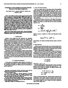
Figure 1: Examples of the circular masks used by SUSAN (adapted from [7]). d

(2)

where λth is a predefined threshold. However, many windows that satisfy the above condition will not contain good features to track, for instance high intensity variations in both directions occur on a slanted edge, however the selected feature may not be unique along the given edge. Some features may also be detected across depth discontinuities; for instance a lamp post makes a distinct corner with a windowsill however both objects move across the image view field at different rates (it was found that this scenario occurred frequently in the automotive environment). Smaller image window sizes are less likely to cross depth discontinuities than larger windows, however if the window is too small, the matrix G is harder to estimate. b) SUSAN Corner detection The SUSAN method is based on circular masks, where each mask has a centre pixel known as the nucleus. The intensity of each pixel within the mask is compared to the intensity of the pixel at the nucleus. If the difference is more than a predefined threshold then the pixel is said to be outside of the “Univalue Segment Assimilating Nucleus” (USAN) area, otherwise the pixel is part of the USAN. Figure 1 shows the USAN masks applied to an image and figure 2 shows the USAN area of the masks applied in figure 1. The USAN area is equal to the area of the circle on a flat featureless surface as shown in figure 2(d). If the nucleus happens to be at a straight edge the USAN area is halved as shown in figure 2(b); if the nucleus is at a corner, it is at its smallest, as shown in figure 2(a), giving the algorithm its name.

a

b

c

Figure 2: The circular masks with the USAN areas in the lighter shade of grey (adapted from [7]).

The SUSAN method is attractive because of its speed and good localisation qualities relative to other corner detection algorithms [8]. III INITIAL COMPARISON A number of initial tests were conducted in order to determine some gross behavioural characteristics of the KLT and SUSAN algorithms. The images were taken with a wide-angle lens. In the first instance, it was found that not all features detected by the KLT method were “good” features to track. Many features that were deemed to be strong features appeared along slanted edges; this is due to pixilation and this effect can vary significantly from frame to frame. Figure 3 shows an example of where this can occur. The features detected by KLT are difficult to track as they can move arbitrarily along the edge of the desk. At the same time, the KLT algorithm did return features from most scenes, however many of them proved very difficult to trace. The tracking algorithm selects the N strongest features based on the minimum eigenvalue criterion, however it is noted that the strongest features were often found not to be the most traceable.

Figure 3: Example of some bad features detected by KLT feature detection

Figures 4 and 5 show typical behaviour of both KLT and SUSAN on a sample image with reasonably well-defined features and corners. In figure 4, the KLT is seen to be effective at determining good features i.e. the corners. However in the presence of slanted edges KLT also detects high variation in both x and y directions, resulting in “features” that are difficult to track. Notice here also that the corners appear in different places in the feature windows which make maintaining good localisation quite difficult. Figure 5 shows the features detected by SUSAN. Only strong well defined corners are detected, however, unlike KLT, “weaker” features may not be detected and the corners detected all appear in the middle of the selected feature window.

Figure 4: Features detected by KLT

Figure 5: Features detected by SUSAN

In the next section we compare the tracking performance of both algorithms. IV TRACKING COMPARISON In this section we discuss and compare the abilities of the tracking algorithms on a real sequence of images taken from the automotive environment using a fisheye camera system. Approximately 20 minutes of video was used for these tests. In Figure 6(a-e) we show some features tracked using the KLT algorithm (indicated by the squares in the images). Both features identified in the frame sequence are in theory good features to track since they both have a high intensity variance in the x and y directions and are located at a corner. However, if we follow the feature on the top of the image sequence we can see that this particular feature is not well localised; in particular, close inspection reveals that the feature window shifts slightly across the feature between frames. This is indicative of many of the features selected by the KLT algorithm in approximately 20 minutes of video taken and processed.

(a)

(e) Figure 6: Features tracked using the KLT tracker

(b) (a)

(c) (b)

(d)

(c)

well as other factors relating to the processing platform used. However, the results presented should give some measure of the relative complexity of the methods.

(d)

(e) Figure 7: Features tracked using SUSAN algorithm

Figure 7 shows features tracked using the SUSAN algorithm (indicated by the green squares in the images) in the same sequence of images as used in figure 6. The features tracked are well localised from frame to frame and the corner is well defined. The sky in the background is a uniform region, providing good contrast for successful corner detection which in turn results in reasonably good tracking.

V COMPLEXITY COMPARISON Apart from their relative performance, another important consideration is the computational complexity of the algorithms. A random sample of sixteen images was processed by both algorithms using MATLAB, with reasonably optimised code. It was found that the KLT took the same amount of time for all images, whereas the SUSAN approach varied depending on the number of corners located in the image. For an image with a large corner count the KLT took as little as 4% of the time the SUSAN algorithm. For an image with a low corner count it took 7% of the time taken by SUSAN, Therefore, if the performance of the KLT can be tolerated there is a strong argument to be made on behalf of the KLT for use in embedded systems (assuming the embedded system has the power required to run the KLT in the first place). It must be recognised that this analysis is limited in the sense that much depends on the degree of optimisation of the code, as

VI DISCUSSION AND CONCLUSION In this paper we have described and compared two feature detection methods, the KLT and the SUSAN corner detection approach, for use in feature detection and tracking applications in the automotive environment. The KLT is capable of detecting good features although it also picks up some features that would be difficult to track, as highlighted in figure 4. Feature localisation was also shown to be poor with the KLT approach, as indicated by the frame sequence in figure 6. On the other hand, the SUSAN algorithm detects corners with good localisation and this advantage carries into the tracker which means that accurate tracking is achieved. However, SUSAN is less effective at detecting “weak” features, therefore, the quality of the image processed by the algorithm is an important consideration. From the point of view of computational complexity, the KLT algorithm appears to have a significant advantage over SUSAN (albeit based on a preliminary analysis), which is an important consideration in embedded implementations. For real-time operation, the KLT probably has an advantage, though there may be a performance penalty with this approach. Future work should involve further validation of the results presented using more extensive test data, as well as a more thorough analysis of computational complexity for embedded implementation. Also, there remains some scope for investigation of a possible combination of the two approaches discussed in this paper where both the KLT and SUSAN are used to detect features drawing a balance between performance and complexity. REFERENCES [1] S.M. Smith and J.M. Brady. Asset-2: Real-time motion segmentation and shape tracking. Transactions of the IEEE on Pattern Matching and Machine Intelligence, vol. 17, number 8, pp 814-820, 1995. [2] S.B. Kang, R. Szeliski, and H.Y. Shum. A parallel feature tracker for extended image sequences. Computer Vision and Image Understanding, vol 67, number 3, pp 296-310, September 1997. [3] J. Shi and C. Tomasi. Good Features to track. IEEE Conference on Computer Vision and Pattern Recognition (CVPR'94), pp 593-600, June 1994. [4] C. Tomasi and T. Kanade. Shape and motion from image streams -- a factorization method. International Journal of Computer Vision, 9(2):137-154, 1992.

[5] C.Tomasi and T.Kanade, Shape and motion form image streams: A factorization method-Part3, Detection and Tracking of Point Features, in Technical Report, 1991, pp CMU.CS.91.132. [6] B..D.Lucas and T. Kanade, An Iterative Image Registsration Technique with an Application to Stereo Vision. International Joint Conference on Artificial Intelligence, 1981, pp 674-679. [7] S.M. Smith and J.M. Brady. SUSAN - a new approach to low level image processing. Int. Journal of Computer Vision, 23(1):45--78, May 1997. [8] W. Wang and R.D. Dony. Evaluation of image corner detectors for hardware implementation. Canadian Conference on Electrical and Computer Engineering, pp1285- 1288 Vol.3 2004.