© by PSP Volume 22 – No 4b. 2013
Fresenius Environmental Bulletin
COMPARISON OF GIS BASED INTERPOLATION METHODS IN ASSESSING OF SITE SPECIFIC PHOSPHORUS VARIABILITY ON THE APPLE ORCHARD M. Rüştü Karaman1,*, Ayhan Horuz2, Tekin Susam3, Fatih Er4 and Ekrem Tuşat4 1
Gaziosmanpasa University, Dept. of Soil Sci. Tokat, Turkey, Ondokuzmayıs University, Dept. of Soil Sci. Samsun, Turkey, 3 Gaziosmanpasa Univ., Dept. of Geodesy and Photogrametry, Tokat, Turkey 4 Selcuk University, Cumra Vocational School, Konya, Turkey 2
KEYWORDS: GIS, Interpolation, semivariogram, geostatistic, phosphorus, apple
ABSTRACT Evaluating of geostatistical approaches in monitoring of spatial variability of some chemical contaminants such as agricultural phosphorus (P) will provide valuable data for large agricultural areas. In this study, performance of varied GIS based geostatistical interpolation methods were tested in assessing of site specific P variability on the apple orchard. For this aim, soil samples were systematically collected from the agricultural apple area using the grid sampling system. The samples were taken at two depths (025 cm and 25-50 cm), the distance on the Y direction is 10 m and in the X direction is 20 m. The soil samples were prepared for analysis, and some physical and chemical analyses were made in the samples by routine methods. The data concerning with soil P levels were analyzed comparatively according to GIS based interpolation methods of Ordinary Kriging (OK), Simple Kriging (SK) and Universal Kriging (UK). The interpolation methods were also tested with varied semivariogram models of Spherical, Exponential and Gaussian. As a result of cross validations, the best optimal method was found to be interpolation method of UK (Universal RMSE, +/- 0.472) with semivariogram model of guassian for topsoil, whereas it was found to be interpolation method of SK (Simple RMSE, +/-0.323) with semivariogram model of exponential for topsoil. Predicted P values were significantly (p< 0.01) correlated with measured values for both topsoil (r = 0.993) and subsoil (r = 0.980), respectively. Soil P distribution maps were adequately performed by using selected kriging interpolation methods and suitable semivariogram models. The results indicated that monitoring of site specific P variability on the apple orchard using these GIS based interpolation methods will help to create the effective schemes for agricultural chemical managements such as P fertilization resulting in optimal yield and quality with reduced environmental pollution.
* Corresponding author
1 INTRODUCTION Crops grown on some soils are less responsive to fertilizer P application, meaning that a great part of the applied fertilizer P will remain in soils as residual part, there will be considerable site specific P variability on the field soils [1-3]. As a matter of fact that many results of studies are available indicating environmental hazards of excess P fertilization such as excessive algae growth in the surface waters and soil pollution associated with phosphate sources having toxic metals, radiation hazards etc. together with unnecessary expenses in the agricultural fields [4-6]. Hence, these mineral fertilizers affect the surface and groundwater quality negatively [7]. On the other hand, adequate soil P levels are important for maintaining uniform growth and yield of crops on the agricultural lands having low available P. Hence, a realistic P budget estimation is required for optimal crop yield and quality with reduced P fertilizer use together with reduced environmental pollution [8]. Site specific monitoring of field soils, that is one of the main step of precision agriculture, provides also more accurate information for balancing P fertilization under the varied soil and plant conditions. Thus, it is generally accepted that a more detailed soil sampling will result in more precise fertilizer recommendations [9]. It has been reported that it was essential to know the spatial variability of soil characteristics and determine the crop nutrient requirements in order to plan a site-specific fertilization program for apples [10]. Recently, various geostatistical interpolation methods have been used to understand the spatial variations and heterogeneities of soil properties on small or large scale parcels to minimize the errors of measured variables [1115]. Interpolation is a mathematical function that estimates the values at locations where no measured values are available [16, 17]. Hence, these applications have proved to solve
1212
© by PSP Volume 22 – No 4b. 2013
Fresenius Environmental Bulletin
complex spatial databases in more precise way. Kriging is an advanced surface creation technique that is most useful when there is a spatially correlated distance or directional bias in the data [18]. Hence, some kriging methods such as ordinary kriging, simple kriging, universal kriging, indicator kriging have been used in order to improve the interpolation accuracy [18-20]. On the other hand, some variograms, which can be used to examine the spatial continuity of a regionalized variable as a function of distance and direction, are also essential step on the way to determining optimal weights for interpolation [21]. The pattern of spatial variability in the form of kriging map may improve the decision for agricultural practices such as fertilizer recommendation rate, which is one of the most important keys for development of site-specific managements. In this study, performance of varied GIS based geostatistical interpolation methods were tested in assessing of site specific P variability on the apple orchard. Evaluating of geostatistical approaches for determining of site specific effects of chemicals such as agricultural P will provide valuable data especially for large agricultural areas. It will be possible to select the best management practices by monitoring agricultural areas with computer based geostatistical models. These approaches will also help to effective fertilization schemes for optimal yield and quality with reduced environmental pollution. The kriging based spatial variation analyses of soil available P will help to better understand the distribution and transport of nonpoint-source P across landscapes and agricultural managements for effective P fertilization schemes resulting in optimal yield and quality with reduced environmental pollution.
concerning with measured values were subjected to the statistical analysis using StatMost package program [23]. TABLE 1 - The summary data concerning with some physical and chemical analysis of soils Soil properties Saturation, % CaCO3, % pH, 1:5 EC, dS m-1 Organic matter, %
Topsoil 67.10 34.90 7.20 0.407 1.90
Subsoil 66.00 46.90 7.62 0.427 1.43
2.3 Descriptive statistics
Descriptive statistics were achieved to provide simple summaries about the sample and about the observations that have been made. For this aim, the coefficient of variance (C.V.), kurtosis and skewness values for site-specific P values of topsoils and subsoils on the apple area were calculated. The Coefficient of variation (CV) expresses the variability of a sample in the units of its mean [24]. It is the ratio of the sample standard deviation to the sample mean;
CV =
s × 100 % x
(1)
A further characterization of the data includes skewness and kurtosis. Skewness measures the degree of asymmetry exhibited by the data. If skewness equals zero, the histogram is symmetric about the mean. Kurtosis characterizes the relative peakedness or flatness of a distribution compared to the normal distribution, and negative kurtosis indicates a relatively flat distribution. 2.4 Geostatistical methods
2 MATERIALS AND METHODS 2.1 Description of study area
This study was conducted on the agricultural apple area located on a flat plain in Konya city (Turkey). The soil texture was clay loam, while the texture of surface layers ranged from clay loam to clay. Soils are generally moderately deep and range in depth from 20 to >100 cm, and it is defined as calcareous soil series. The grid sampling based on 20 m x 10 m was selected for this study because grid sampling reduces a large degree of uncertainty. 2.2 Sampling methods
Fourty five soil samplings were taken at depths (0-25 cm and 25-50 cm), the distance on the X direction was 20 m and on the Y direction it was 10 m. A 9x5 grid spaced is 10 m apart East and 20 m apart North. The soil samples were taken using a stainless steel soil auger, and three soil cores from each depth were taken and mixed together to obtain one sample at each point. The soil samples were air dried and ground to pass through a 2-mm sieve for analysis in the laboratory. In the experimental soil, available P was determined by the method of Olsen et al. [22]. Some other physical and chemical analyses were made in the samples by routine methods (Table 1). Experimental data
Geostatistical analyses of research data were studied by Geostatistical analyst module of ArcMap 9.3.1. GIS software by ESRI [25] were used for predicting the spatial structure of soil P levels. To achieve cross-validation, distribution percentages were formed by using kriging interpolation methods. The data concerning with topsoil and subsoil P were analyzed comparatively according to interpolation methods of Ordinary Kriging (OK), Simple Kriging (SK) and Universal Kriging (UK). The interpolation methods were also tested with varied semivariogram models of Spherical, Exponential and Gaussian in order to comparing. The semivariogram was defined as: γ(si,sj) = ½ var (Z(si) - Z(sj)), where var was the variance, Z(Si), the prediction value, Z(si), the actual value of the validating point. Computation of a variogram involves plotting the relationship between the semivariance (γ(h)) and the lag distance (h) [26]. In variogram, this arises as nugget variance “Co”. The spatial variability variogram stops its increase after a certain distance and the peak variance (sill) starts having values around “Co+C”. The distance at which the variogram reaches the sill value is named as the effect area or range “a”. The value that the semivariogram model attains at the range (the value on the y-axis) is called the sill. The partial sill is the sill minus the nugget. The nugget effect can be attributed to measurement errors or spatial sources
1213
© by PSP Volume 22 – No 4b. 2013
Fresenius Environmental Bulletin
of variation at distances smaller than the sampling interval or both [27]. The ratio between nugget semi-variance and total semi-variance or sill was used to define different classes of spatial dependence. If the ratio was less than 25, the variable was considered to be strongly spatially dependent, or strongly distributed in patches; if the ratio was between 26 and 75, the variable was considered to be moderately spatially dependent; and if the ratio was greater than 75, the variable was considered weakly spatially dependent [28]. To compare interpolation results, the values of Mean Error (ME) and Root Mean Squared Error (RMSE) were used. The RMSE was a measure of prediction performance of the varied interpolation methods. The ME and RMSE was calculated using the following equation [21];
ME
RMSE
=
1 2 =
n
∑ [Z (S ) − z (s )] i
i=1
1 n
(2)
i
∑ [Z (S ) − z (s )] n
2
i
i=1
i
(3)
Where : Z(Si): the prediction value, Z(si): the actual value of the validating point I, n: the number validation points, ME: Mean prediction error, RMSE: Root mean square error i : a validating point and si: the position of validating point i. Three dimensional distribution maps obtained for the related elements as a result of the interpolation made by using the chosen kriging method and the semivariogram model were presented for the experimental points. 3 RESULTS AND DISCUSSION The coefficient of variance (C.V.), kurtosis and skewness values for site-specific P values of topsoils and subsoils on the apple area were calculated. As it is seen from Table 2, available P values were varied from 1.08 to 19.67 kg P da-1 for topsoil, whereas it was varied from 0.69 to 9.27 kg P da-1 for subsoil. The coefficient of variance (C.V.), kurtosis and skewness values also indicated that a great spatial variability occurred for selected site specific P values of the soils (Table 2). Positive kurtosis values of 4.16 and 0.75 were determined for topsoil and subsoil, which characterizes the relative peakedness or flatness of a distribution compared to the normal distribution. The maximum C.V. value of 56.39 % was measured for available P value in the subsoil. The C.V. value of 25.78 % was also determined for topsoil. It has been classified the C.V. values as 0-15 (low),
16-35 (medium) and 36 < (high) variable, respectively [29]. In a similar work, a quite high coefficient of variation (C.V. 31 %) for Olsen’s P values has also been found suggesting that there was a high P variability within cotton field [9]. Many other studies have also revealed that a great spatial variability of soil P was determined depending on varied factors [30-32]. Field scale variability of soil P was also observed for other plants [33, 34]. On the other hand, the results further indicated that available P deposited existed in the subsoil. In a similar study conducted on a sugarbeet field, the highest C.V. value of 41 % was also found for subsoil P, whereas it was 34 % for topsoil P, meaning that subsoil P accumulation was higher than topsoil P [35]. Thus, deep plowing could be performed every four to five years to mix P from this source with the topsoil and enhance P uptake by the crop. TABLE 3 - Theorical models testing for soil P values and RMSE errors Model ME* RMSE** ASE*** Topsoil Universal Kriging Spherical 0.1963 0.6469 0.9018 Exponantial 0.2053 0.6751 1.1430 Guassian 0.1415 0.4722 0.6644 Subsoil Simple Kriging Spherical 0.0191 0.3522 0.4381 Exponantial 0.0255 0.3238 0.4564 Guassian 0.0009 0.4839 0.5290 *Mean Prediction Error (ME) should be near zero, **Root Mean Square (RMSE) is a measure of prediction performance of the varied interpolation methods. ***Average Standart Error (ASE) should be close to 1
Geostatistical parameters of site specific soil P levels for topsoil and subsoil were presented Table 3 and 4. The data for site specific soil P levels were analyzed through kriging methods of UK and SK, which are the computer based geostatistical interpolation methods. As a result of cross validations, the best optimal interpolation and semivariogram model with the lowest RMSE have been obtained by UK method and Gaussian semivariogram model with RMSE = +/- 0.472 for data group concerning with topsoil P levels. Whereas, the best optimal interpolation and semivariogram model with the lowest RMSE have been obtained by SK method and exponential semivariogram model with RMSE = +/- 0.323 for subsoil (Table 2). Average mean and standard deviations for measured and predicted values were indicated that the standard deviations of predicted values were nearly similar to the standard deviations of measured values. Predicted P values were significantly (p75 weakly spatially dependent (W)
In this study, nugget effect of 0.2573 was determined for topsoil, whereas it was 0.5509 for subsoil based on UKguassian and SK-exponential, respectively. Values of the relative nugget effect near 1.0 indicate that a large degree of the variability is associated with the within sample measurements, and that relatedness between spatially separated measurements is limited. A relative nugget effect near zero indicates that the relatedness of spatially separated measurements within the range is strong. The range represents the “zone of influence of the sample” [37,38]. On the other hand, based on nugget/sill ratio of < 25, strongly dependences were observed for both topsoil and subsoil P values. According to the selected kriging method and semivariogram models, soil P levels were spatially varied at short distance within the study area. The maximum range was 18.57 m for topsoil P levels, whereas it was 21.98 m for subsoil P levels. It has also found that soil test P, K and pH generally had smaller ranges while total N and
High: 18,65 Low: 1,26
FIGURE 1 - Spatial distribution faces of topsoil P levels performed using the interpolation method of UK
High: 8,75 Low: 0,85
FIGURE 2 - Spatial distribution faces of subsoil P levels performed using the interpolation method of SK
1215
© by PSP Volume 22 – No 4b. 2013
Fresenius Environmental Bulletin
organic C tended to be larger [38]. They have concluded that at least some of the variables measured in that study had displayed trends at distances separating measurements of about 10 m, whereas samples collected at 50 m or larger intervals would miss short distance changes in the values of soil variables. In other work, it have have been reported that correlations that occur most strongly at shorter distances and weaken with increasing distance indicate that spatially continuous data, including most soil properties, are strongly positively autocorrelated [39,40]. Spatial distribution faces of soil P levels performed using the interpolation methods of UK and SK were presented Fig. 1 and Fig. 2. The dipping variances on the distribution faces are to indicate a trend, which were detrended in the data. 2D kriging surfaces, which is height of the variable and processed by geostatistical analyst module, have also clearly indicated soil P variability borders on the apple orchard. The borders for available soil P can be nearly classified; < 3 kg P da-1 is insufficient, whereas 3 kg P da-1 < is sufficient or excess levels for apple growth based on the fertilization guide [41].
REFERENCES [1]
Bronson, K.F., Keeling, J.W., Booker, J.D., Chua, T.T., Wheeler, T.A., Boman, R.K. and Lascano, R.J. (2003). Influence of landscape position, soil series, and phosphorus fertilizer on cotton lint yield. Agronomy Journal, 95,949-957.
[2]
Ganawa, E.M., Soom, M.M., Musa, M.H., Shariff, A.M. and Wayayok, A. (2003). Spatial variability of total nitrogen and available phosphorus of large rice field in Sawah Sempadan Malaysia. Science Asia 29:7-12.
[3]
Karaman, M.R., Şahin, S., Çoban, S. and Sert, T. (2005). Site specific phosphorus status of wheat plants (Triticum aestivum) on calcareous Soils. Journal of Revue De Cytologie Et Biologie Végétales. 28:128-134, France.
[4]
Sharpley, A., Daniel, T.C., Sims, J.T. and Pote, D.H. (1996). Determining environmentally sound soil phosphorus levels. Journal of Soil and Water Conservation 51(2):160-166.
[5]
Sims, J.T., Simard, R.R. and Joern, B.C. (1998). Phosphorus loss in agricultural drainage: Historical perspective and current research. J. Environ. Qual. 27:227-293.
[6]
Börling, K., Otabbong, E. and Barberis, E. (2003). Soil variables for predicting potential phosphorus in Swedish Noncalcareous Soils. Ecologicl Risk Assesment. J. Environ. Qual. 33:99-106.
[7]
Demirel, Z., Özer, Z. and Özer, O. (2010). Nitrogen and phosphate contamination stress of groundwater in an internationally protected area, the Göksu Delta, Turkey. Fresenius Environ. Bull. 19, 2509-2517.
[8]
Hedley, M.J., Mortvedt, J.O., Bolan, N.S. and Syers, J.K. (1995). Phosphorus Fertility Management in Agroecosystems. In: Phosphorus in the Global Environment, Transfer, Cycles and Management. pp. 59-92, Tiessen, H. (Ed.), Wiley Press, Chichester, UK.
[9]
Dikici, H. and Gundoğan, R. (2002). Measuring within field variability for phosphorus: A Site Specific Approach. International Conference On Sustainable Land Use And Management, September, Çanakkale, Turkey.
4 CONCLUSIONS The results showed that measured soil properties like P levels could be spatially vary within a short distance. Thus, the study clearly revealed that convensional soil sampling methods based on only average samplings for large fields will lead to very high or low P fertilizer recommendations for the crops, which also means highly P accumulation on the agricultural lands resulting in environmental problems. The experimental data concerning with soil P levels were also analyzed comparatively according to GIS based interpolation methods of Ordinary Kriging (OK), Simple Kriging (SK) and Universal Kriging (UK). The interpolation methods were also tested with varied semivariogram models of Spherical, Exponential and Gaussian. As a result of cross validations based on RMSE values, the best optimal method was found to be interpolation method of UK with semivariogram model of guassian for topsoil, whereas it was found to be interpolation method of SK with semivariogram model of exponential for topsoil. Predicted P values were significantly correlated with measured values for both topsoil and subsoil, respectivly. Soil P distribution faces were adequately determined by using selected kriging interpolation methods with suitable semivariograms for the experimental data group, respectively. The results have revealed that testing the performance of spatial interpolation techniques for mapping soil properties could improve the decision support for field management practices. Thus, site specific P variability on the apple orchard using these GIS based interpolation methods will help to create the effective schemes for agricultural chemical managements such as P fertilization resulting in optimal yield and quality with reduced environmental pollution
1216
[10] Aggelopoulou, K.D., Pateras, D., Fountas, S., Gemtos, T.A. and Nanos, G.D. (2011). Soil spatial variability and sitespecific fertilization maps in an apple orchard. Precision Agric., 12:118-129. [11] Yost, R.S., Uehara, G. and Fox, R.L. (1982). Geostatistical analysis of soil chemical properties of large land areas. I. Semivariograms. Soil Sci. Soc. Amer. J., 46:1028-1032. [12] Bo, S., Shenglu, Z. and Qiguo, Z. (2003). Evaluation of spatial and temporal changes of soil quality based on geostatistical analysis in the hill region of subtropical China. Geoderma, 115:85-99. [13] Stamatopoulou, I.G., Mitsios, I.K., Floras, S. and Zerba, G. (2003). Study of spatial variability of available potassium, calcium, magnesium and sodium in central Greece using geostatistics. Geographical Information Systems and Remote Sensing: Environmental Applications. Proceedings of Int. Symp., 07-09 November. [14] He, Y., Song, H., Zhangand, S. and Fang, H. (2005). Study on the spatial variability and the sampling scheme of soil nutrients in the field based on GPS and GIS. Proceedings of the IEEE Engineering in Medicine and Biology 27th Annual Conference Shanghai, China, Sept., pp. 1-4.
© by PSP Volume 22 – No 4b. 2013
Fresenius Environmental Bulletin
[15] Ren, C., Wang, Z., Song, K., Zhang, B., Liu, D., Yang, G. and Liu, Z. (2011). Spatial variation of soil organic carbon and its relationship with environmental factors in the farming-pastoral ecotone of Northeast China. Fresenius Environmental Bulletin. Fresenius Environ. Bull. 20, 253-261. [16] Robinson, T.P. and Metternicht, G. (2006). Testing the performance of spatial interpolation techniques for mapping soil properties. Comput. Electron. Agr. 50:97-108. [17] Gao, Y., Junfeng, G. and Chen, J. (2011). Spatial variation of surface soil available phosphorous and its relation with environmental factors in the Chaohu Lake Watershed. Int. J. Environ. Res. Public Health, 8:3299-3317. [18] Heuvelink, G.B.M. and Bierkens, M.F.P. (1992). Combining soil maps with interpolations from point observations to predict quantitative soil properties. Geoderma, 55:1-15. [19] McBratney, A.B., Santos, M.L.M. and Minasny, B. (2003). On digital soil mapping. Geoderma, 117:3-52. [20] Zhengyong, Z., Chow, T.L., Rees, H.W., Yang, Q., Xing, Z. and Meng, F.R. (2009). Predict soil texture distributions using and artificial neural network model. Computers and Electronics in Agriculture, 65:36-48. [21] Burrough, P.A. and McDonnell, R.A. (1998). Principles of geographical information systems, Oxford University Press, 333 pp, U.K. [22] Olsen, S.R., Cole, C.V., Watanable, F.S. and Dean, L.A. (1954). Estimation of available phosphorus in soils by extraction with sodium bicarbonate. Agricultural Handbook, U.S. Soil Dept. 939, Washington D.C. [23] StatMost, (1995). Dataxiom Software Inc. User’s Guide: StatMost. 5th Ed. Dataxiom Soft. Inc., LA., USA. [24] Vidakovic, B. (2011). Statistics for bioengineering sciences with MATLAB and WinBUGS support, 753 p. 190 illus in color, ISBN: 978-1-4614-0393-7, Hardcover, Springer.
[33] Buzas, I., Tamas, J. and Cserni, I. (2003). Correlation between yield and soil characteristics in a heterogenous field. 14th International Symposium of Fertilizers. Proceedings Book, pp. 57-67, June 22-25, Debrecen, Hungary. [34] Mesterhazi, P.A., Nemenyi, M., Kovacs, A., Kacz, K. and Stepan, Z. (2003). Development of the technical environment of the site-specific nutrient replacement. 14th International Symposium of Fertilizers. Proceedings Book, pp. 288-295, June 22-25, Debrecen, Hungary. [35] Karaman, M.R., Susam, T., Yaprak, S. and Er, F. (2009). Computer based geostatistical strategies in assessing of spatial variability of agricultural phosphorus on a sugarbeet field. ICIME, 13:201-205. [36] Rivero, R.G., Grunwald, S. and Bruland, G.L. (2007). Incorporation of spectral data into multivariate geostatistical models to map soil phosphorus variability in a Florida wetland. Geoderma, 140: 428-443. [37] Knighton, R.E. and Wagnet, R.J. (1987). Geostatistical estimation of spatial structure. In Continuum, Vol:1. Ithaca, N.Y.: Water Resources Inst., Center for Environ. Res. [38] Solie, J.B., Raun, W.R. and Stone, M.L. (2001). Submeter spatial variability of selected soil and plant variables. Soil Sci. Soc. Am. J. 63:1724-1733. [39] Bailey, T.C. and Gatrell, A.C. (1995). Interactive Spatial Data Analysis (Addison Wesley Longman Limited, Essex, England), pp. 162-166. [40] Kozar, B., Lawrence, R. and Long, D. (2002). Soil Phosphorus and Potassium Mapping Using a Spatial Correlation Model Incorporating Terrain Slope Gradient. Precision Agriculture, 3:407-417. [41] Ülgen, N. and Yurtsever, N. (1995). Turkish Fertilizer and Fertilization Guide. Soil and Fertilizer Research Institute, General Publication No:209, Ankara.
[25] ESRI, (2005). Geostatiscial Analysis Module Hand Book. ESRI Inc. Publication, The Netherland. [26] Lacozza, J. and Barber, D. (1999). An examination of the distribution of snow on Sea-Ice. Atmosphere-Ocean, 37(1):2151. [27] Anonymous, (2012). Understanding a semivariogram: The range, sill, and nugget. http://resources. arcgis.com/en/home/ [28] Cambardella, C.A., Moorman, T.B., Novak, J.M., Parkin, T.B., Karlen, D.K. and Turco, R.F. (1994). Field-scale variability of soil properties in central Iowa soils. Soil Science Society of America Journal, 58:1501-1511. [29] Webster, R. (1985). Quantitative Spatial Analysis of Soils in The Field. Advances in Soil Science, Volume: 3. SpringerVerlag, New York, 3-69 pp. [30] Grunwald, S., Reddy, K.R., Newman, S. and DeBusk, W.F. (2004). Spatial variability, distribution and uncertainty assessment of soil phosphorus in a south Florida wetland. Environmetrics, 15:811-825. [31] Vaughan, R.E., Needelman, R.A., Kleinman, P.J.A. and Allen, A.L. (2007). Spatial variation of soil phosphorus within a drainage Ditch Network. J. Environ. Qual. 36:1096-1104. [32] Zhang, Z.M., Yu, X.X. and Li, J.W. (2010). Spatial variability of soil nitrogen and phosphorus of a mixed forest ecosystem in Beijing, China. Environ. Earth Sci. 60:1783-1792.
1217
Received: July 30, 2012 Revised: October 02, 2012 Accepted: November 12, 2012
CORRESPONDING AUTHOR Prof. Dr. M. Rüştü Karaman Gaziosmanpasa University Agricultural Faculty Head of Department of Soil Science Tokat TURKEY E-mail:
[email protected] [email protected] FEB/ Vol 22/ No 4b/ 2013 – pages 1212 - 1217