(1989), George and Liu (1981), or my class notes (Misztal ..... Comments by Drs. George Wiggans and Curt. Van Tassel are gratefully appreciated. Several.
Complex Models, More Data: Simpler Programming? Ignacy Misztal University of Georgia, Athens, GA 30602, USA.
1. Introduction
2. Software complexity and Optimization
The complexity of models used for or considered for use in genetic evaluation is increasing. Examples of new models are test-day models in dairy cattle, growth models in beef cattle, and models with dominance or/and QTL effects. These models are usually linear but analyses of some traits may require nonlinear models, which are usually more complicated to write and test. More complicated models may require a larger data set. In the future we may expect new types of models that will be used to analyze even larger data sets. In order to support new models, the computer programs need to be upgradeable and therefore easy to understand or simple. Programs in a matrix language are usually simple but inefficient and cannot work with larger data sets. In order to support large data sets, programs need to be efficient, which usually means complicated and hard to modify. Traditionally, mixed model packages available in animal breeding were written with efficiency in mind. Although they are useful at a time when they are developed, they become outdated. For example, none of the packages available in 1994 (Misztal, 94) supported the now-popular random regressions. Some of these packages have been updated to include random regressions, but some may be too complicated to update. Two developments can lead to simple yet efficient programs: increase in computer power and programming languages with objectoriented features. Greater computer power allows avoidance of optimizations that would complicate programs. Better programming languages allow to express the same algorithms simpler but as efficient.
Software complexity is a function of the number of variables, subroutines, and subroutine interfaces. A large number of variables and subroutines increases the time to learn meaning of each variable and subroutines, and makes it easier to confuse them. A large number of parameters in each subroutine/function makes it hard to understand their functionality and makes undesirable side effects more likely. Time to learn decreases if names in programs have intuitively obvious purpose and the program flow is clear. Time to learn increases if optimization makes the programs flow complicated. Time to learn does not increase if an operation with large complexity is hidden either in the system or in the library. For example, very complex algorithms may implement arithmetic operations in a matrix language, but the user is not involved in learning them. In programs, the majority of time is usually spent in a few areas called the bottlenecks. In REML programs, bottlenecks are sparse matrix factorization and inversion. In programs solving by iteration on data, reading the data repeatedly could use 95% of the time. In Gibbs-sampling type of programs, the majority of time can be spent in updating the mixed model equations repeatedly. For each of these applications, it makes sense to optimize their bottlenecks only and keep other parts of the program as simple as possible. As shown later, the bottlenecks can be encapsulated into modules to make them appear simple.
2 3. Opportunity from Hardware Improvements According to Moore’s law computer power increases doubles every 18 months. This increase results from faster processor speed, increased memory and disk capacity. A dualPentium with 1024 Mbytes of memory cost about $5000 in 1998. IBM 3090 with similar capabilities in 1988 could cost 1000 times more. Some of the new computer power could be used to eliminate optimizations that make programs more complicated. For example, availability of larger memory reduces the need for memory optimization by allowing to use simpler but more memory intensive algorithms. Current computers utilize memory hierarchies, with a very fast on-chip cache memory and a relatively slow external memory. Operations with data that fit into the cache are much faster than that those that require external memory. Subsequently, low-level optimizations such as pre-inverting residual (co)variance matrices or in-lining subroutines are not as important as before. Large disk space makes coding to conserve disk space less critical.
4. Programming Languages Previously, most programming in animal breeding has been done in Fortran 77 (F77). This language leads to efficient but complex programs. Because of few control and data structures available, non-numerical computing required programming “tricks“, which made programs in F77 even more complicated. Computer language C has also been used in animal breeding. It has a richer collection of data and control structures but also involves more details and may be less convenient and efficient for numerical computing. Currently, programming moves towards object oriented languages. Two features of such languages are especially useful to reduce complexity. First, encapsulation allows packaging of complicated operations on complicated data structures into
libraries/classes/modules. Details of operations in the module can be hidden from the user. Subsequently, the number of arguments in subroutine/function names can be fewer. For example, operations on matrices would not have to involve dimensions of the matrix, or in sparse matrices, implementation details. Second, overloading, the use of a single function/subroutine name with logically similar but physically different data structures, can be used. For example, the same subroutine name can be used to print matrices in single or double precision, and in full or half-storage. Overloading allows a reduction in the number of subroutine/function names to remember, and it allows better diagnostics. The most popular programming language with object oriented features at this time is a follower of C, C++. This language is refined and free compilers are available. C++ also has an overwhelming number of features, but it does not allow easy use of old but tested Fortran subroutines. A very comprehensive package in C++ for mixed model and statistical computations called MATVEC has been developed by Wang (personal communication, 1994). Due to a number of issues including problems related to its large size, MATVEC has not been officially released. Another language with object-oriented features is a follower of F77, Fortran 90 (F90). It’s new data and control structures now match those of C, as it supports data structures, pointer and allocatable arrays, and endless loop and case statements. Matrix operations result in simpler code, and internal functions allow easy decomposition of the main program into logically independent blocks. Interfaces allow the reduction in the number of parameters passed to subroutines and to use one subroutine name for one operation with different data types. Complex operations can be packaged into modules, where the program complexity is hidden from the user. Besides a range of new features, F90 language supports old F77 subroutines/functions. Thus, if efficient and reliable subroutines exist in F77, they can be
3 adopted into fortran 90 programs directly, or even better, wrapped into F90 code to make their use much easier.
5. Design of BLUPF90 BLUPF90 is a mixed model program written in Fortran 90. This program was developed step by step in my graduate level course initially as a teaching tool but soon was generalized into a research tool. The design goals were: 1) support for a large range of models, 2) easy extensibility if necessary, 3) new code programming in Fortran 90, 4) maximum use of legacy Fortran 77 subroutines/functions via modules, 5) avoidance of proprietary code in subroutines/functions. All variables and constants necessary to describe a model are defined in a module model. There, each effect is either a cross-classified variable, covariable, or nested covariable. For simplicity, in multiple traits, the equations are blocked within traits. Each effect needs to be defined for each trait but the same effect can have a different design for each trait. In particular, an effect with a “null“ design matrix results in support for different models by trait. Multiple groups of correlated random effects
are allowed. Each group includes one or more random effects and is one of the following types: additive sire-maternal-grandsire, additive animal with options for unknown parent groups and inbreeding, and parental dominance. Groups of random effects are independent, and two groups of random effects with the same type are possible. This is useful, for example, in some crossbreeding models, where support for two or more different additive effects is needed. Generality of random groups enables new types of models, as for example a random regression model with dominance effect and support for crossbred populations. Solutions in BLUPF90 were obtained by the following methods: by successive over relaxation (SOR) iteration within memory or by sparse matrix package FSPAK. For simplicity, all large-matrix manipulation is encapsulated in modules SPARSEM and FSPAK90.
6. Modules Module SPARSEM Module SPARSEM includes definitions of data structures and functions and subroutines to manipulate on these structures. Four matrix formats are available.
Name
Type of Matrix
Comments
DENSEM DENSE_SYMM
dense square dense symmetric; upper-stored
SPARSE_HASHM
symmetric sparse triple accessed by hash algorithm; upper-stored symmetric Sparse IJA; upper stored
easy operations approximately only half memory requirements of the dense square efficient format for set-up and for iterative-solving of sparse matrices
SPARSE_IJA
memory-efficient format for sparse matrices used by sparse matrix packages; cannot be set up directly
4 For more information on these formats see Duff et al. (1989), George and Liu (1981), or my class notes (Misztal, 1999). A popular format that is not included here is linked list. This format is efficient for creating and computing with sparse matrices provided that the number of nonzero elements per row is not too high and the matrix is not too large. However, the combination of HASH plus IJA is generally more efficient. To create a particular matrix structure, let the program know to use the sparsem module, and then decleare a variable: Program ABC use sparsem ............... type (densem)::A As declared, the structure takes only a minimal amount of storage. Matrices are manipulated mainly via subroutines and functions in SPARSEM. To initialize and zero a matrix of n x n: call zerom(A,n) This will initialize the internal structure of whatever format A was defined. If matrix A was initialized previously to a different dimension, it is reinitialized. To add a scalar p to Aij , use
Formats of matrices can be changed without changing the remainder of the code, just by changing the type of matrix A. If a matrix A is defined as DENSEM, the largest matrix that can be stored in 200 Mbytes is 5000 x 5000. If A is changed to SPARSE_HASHM, the largest matrix that can be stored will depend on its sparsity but it could be 1,000,000 x 1,000,000 or larger. Structure SPARSE_IJA cannot be set up efficiently. It can be converted to SPARSE_HASHM as follows: type (sparse_hashm) ::A type (sparse_ija)::A_ija .... call zerom(A,n) .... call addm(...,A) .... A_ija=A Conversions between all the formats involve only (=). Please note that the explicit initialization of A_ija is not needed as it is done during the conversion. Many other operations useful in animal breeding research have been defined, such as selecting matrix blocks from matrices, computing quadratic forms or traces, setting and accessing individual elements of a matrix, and printing.
call addm(p,i,j,A) Finally, assuming that the matrix A as well as the vector of right hand sides b are set up, the solution to the system of equations: Ax=b can be obtained by iteration: call solve_iterm(A,b,x)
Sparse matrix module SPARSEOP (FSPAK90) FSPAK (Perez-Enciso et al., 1994)) is a popular choice in animal breeding for sparse matrix factorization and inversion as well as calculation of the determinant. Unfortunately, it is also difficult to use. To solve and obtain a sparse inverse, the following was needed:
5 integer m1/100000/,& m2/100000/,& m3/200000/
! guess maximum number of equations ! guess number of nonzero elements ! guess maximum amount of working storage
integer ia(m1+1),ja(m2) real*8 a(m2) integer mem(m3)
! declare components of IJA structure ! declare working storage
! ordering call fspak(10,n,ia,ja,a,sc,flag,6,99,mem,mem_needed,work,i,..,rank_o) ! symbolic factorization call fspak(20,n,ia,ja,a,sc,flag,6,99,mem,mem_needed,work,i,..,rank_o) ! solve call fspak(50,n,ia,ja,a,sol,flag,6,99,mem,mem_needed,work,i,..,rank_o) ! sparse inverse call fspak(61,n,ia,ja,a,sc,flag,6,99,mem,mem_needed,work,i,...,rank_o) FSPAK90 (Misztal and Perez-Enciso, 1998) is a Fortran 90 interface to FSPAK that accepts matrices in SPARSE_IJA format and handles sequencing of operations, allocation of memory and error handling. The code below is equivalent to the code above: type (sparse_hashm):: x .... call fspak90(x,’inverse’) FSPAK has a few other options, many of which use optional arguments. call fspak90(’solve’,A,b,x) call fspak90(’det’,ija,det=d) call fspak90(’ldet’,ija,det=ld) call fspak90(.....,rank=r) call fspak90(’factor’,ija) call fspak90(‘reset’)
! solve system AX=b ! obtain determinant d ! obtain log determinant ld ! obtain rank r with any operation ! force new factorization ! deallocate internal memory
Other Modules Module IOUNF Module IOUNF automates fast unformatted I/O necessary for implementations of iteration on data algorithms. For every unit opened, a large buffer is created within IOUNF. When small vectors are written to or read from IOUNF, transfers involve mostly the buffer. Actual I/O transfers occur only when the buffer is empty for reading or full for writing. Many units can be opened simultaneously. For typical reads, IOUNF could be 10 times faster than formatted I/O and 3 times faster than unformatted transfers of small vectors. Module IOUNF could be used as shown below.
6 use iounf .... call iob(iob_open,8) ... call iobuff(iob_write,8,x) ... call iobuff(iob_rewind,8) .... call iobuff(iob_read,8,x,stat=status) .... call iobuff(iob_delete,8)
! unnamed file attached to unit 8 ! write x to unit 8 ! rewind unit 8 ! write, status #0 if end of data ! erase file
Module Gibbs Module GIBBS provides basic operations for Gibbs sampling. These include: a) functions generating multivariate normal and inverted Wishart distributions that also work for scalar arguments, b) subroutines to fast update the coefficient matrix of the mixed model equations, and c) subroutines to solve and update by blocks of equations. An example of a code with module GIBBS is shown below. use gibbs ! setup mixed model equations ! convert matrix in format sparse_hashm to sparse_ija using links call link_hash_ija(xx,xx_ija) ! generate random samples for effects do i=1,neq,ntrait firsteq=(i-1)*ntrait+1; lasteq=i*ntrait call solve_iterm_block(xx_ija,xy,sol,firsteq,lasteq,diag,’solve’) sol(firsteq:lasteq)= & gen_normal(sol(firsteq:lasteq),inverse(diag)),seed1) call solve_iterm_block(xx_ija,xy,sol,firsteq,lasteq,diag,'update') enddo ! generate random samples for variance components (except residuals) ... g(i,:,:)=gen_invwishart(g(i,:,:),df,seed2) ... Module DENSEOP Module DENSEOP implements matrix operations on dense general and symmetric matrices. Each subroutine/function is overloaded to work with several types of arguments. This
module is primarily designed for matrix operations where timing and memory requirements are not critical. For symmetric matrices, each of the functions/subroutines accepts full-stored and packed (half-stored) matrices. Each matrix or
7 vector can be in single or double precision. However, in one function/subroutine, all arguments need to be of the same precision, and all matrices should be stored the same way. For symmetric matrices , the following subroutines are defined : call chol(A,rank) Cholesky decomposition call inverse_s(A,rank) Generalized inverse: -
AI = A
call eigen(A,d,V) Eigenvalues and eigenvectors: A =V diag(d) V’ call solve_s(A,b,x) Generalized solutions x: Ax=b
Optional variable rank returns the rank of the matrix. Most of the subroutines are also available as functions: fchol(A) finverse_s(A) fsolve_s(A,b) fdet(A)
Cholesky decomposition Generalized inverse Generalized solve Determinant of A
For general matrices, the following subroutines and functions are available: call inverse(A) call solve(A,b,x)
Inverse: AI = A-1 Solve x: Ax=b
AI=finverse(A) x=fsolve(A,b)
Returns inverse: AI = AComputes x: Ax=b
Finally, printing of any of the formats supported by DENSEOP is done by:
such by setting negative eigenvalues to .0001 (or optionally min_eig) times the largest eigenvalue, and optionally by printing a message text and by setting status=.true. A=diag(d) d=diag(A)
makes diagonal matrix extracts diagonal elements
Development of the DENSEOP module raised issues of how to obtain low-level software for dense matrices and for calculations of eigenvalues and eigenvectors. Subroutines from Numerical Recipes (Press et al., 1992) would be sufficient and compact, but they are not in public domain. We eventually decided to use appropriate routines from LAPACK90 (Miller, 1999). However, after eliminating unnecessary code, these routines consisted of almost 10,000 lines of code as opposed to about 300 from Numerical Recipes (Press et al., 1992). In the past, this large size would be a major issue because of long compilation time and increases in executable codes. Now, however, with fast compilers and large disks, we view the selection of LAPACK90 as an acceptable choice. In Fortran 90, internally a separate routine is needed for each different matrix format. With four types of matrices, one needs to replicate one routine 4 times. In DENSEOP, all computations are done with double precision fully-stored matrices, and operations involving other formats are supported by conversions.
call printmat(matrix, text, fmt)
7. Programs
which prints any type of matrix using the specified format fmt and preceded by text. Both text and fmt are optional. The following subroutines and functions operate on only double precision arguments and full-stored matrices:
The initial goal for the project was a BLUP program called BLUPF90 that calculated mixed-model solutions only using equations stored in memory. To reduce the complexity, no attempts were made to create a superpackage, but different versions of the same program have been created for different tasks. REMLF90 was created for estimation of variance components using the EM REML algorithm (Dempster et al., 1977) with acceleration. BLUP90THR is a
call pos_def(A,text,min_eig,status) If A is not semi-positive definite, it makes it
8 bivariate linear-threshold model. BLUP90IOD is an iteration on data program that uses a preconditioned conjugate gradient. The last algorithm as documented for animal breeding by Lidauer and Stranden (1998), is an ideal match for this family of programs because it is very simple yet reliable and fast. All of the mentioned programs are functional but are being improved. For example, REMLF90 is being upgraded to support the Average Information (Jensen et al, 1997) algorithm.
8. Experiences Modules and programs Initial development of the SPARSEM library was fast mainly because the implementation for the DENSEM format was easy using f90 matrix operations. Subsequently, testing information was available for the remaining formats. Debugging the BLUPF90 program was also fast. Development of REMLF90, which was created mainly by adding a subroutine REML to BLUPF90, was more complex for several reasons. In multiple traits, it was found that unsymmetric blocks of symmetric matrices are not correctly extracted in sparse matrix formats. A complete extraction was deemed to expensive to implement in format SPARSE_IJA, and separate functions to extract a block and then create a trace were replaced by one combined function. Later, a memory leak was found, which caused the program to allocate more memory each round. Such problems are common to programs that use pointer variables with dynamic memory allocation. However, the majority of development time was spent in understanding formulas for residual variances in EM REML; such formulas are quite complicated when traits are missing (Mantysaari and VanVleck, 1988 ). Another problem was found during the development of the threshold-linear program. An out-of bound access of an array local to a routine that calculated thresholds caused
SPARSEM to crash. Thus the modules may not be immune from programs that use them. Occasionally, problems were associated with the modules. In such cases, a problem could be caused by incorrect arguments passed to a function or subroutine in a module (need better diagnostics), by incomplete understanding of functionality of a module (need better documentation), or by a bug. Currently, the modules have only minimal diagnostics. While programming using modules seems to be relatively easy, localizing and correcting a bug in a module can be a major undertaking. This underscores the need for the availability of software support as well as the need for documentation on internals of each module. Hopefully, with time the modules will become relatively error free and better documented. Fortran 90 Compilers The code was initially developed under MSDOS and later continued under various Unix systems including Linux. Initially, many different problems were encountered with different compilers, but most of these problems disappeared when compilers were upgraded to the latest version. In one case, a compiler bug required a separate version of the FSPAK90 module. When purchasing a compiler for serious development in Fortran 90, it is important to select a vendor with good customer support so that problems that appear to be compiler related can be diagnosed rapidly. Efficiency In the BLUPF90 program, the bottleneck was the solution routine, which was optimized as a low level subroutine. Thus, no extra optimization was needed. The same was true in the REMLF90 program, where the bottleneck was in sparse matrix factorization and inversion by FSPAK. When BLUPF90 was converted to iteration on data using preconditioned conjugate gradient with fast I/O by IOUNF, the majority of the CPU time was spent in a function
9 calculating addresses of equations. Simple optimization to this function cut the running time in half. Further optimizations were hampered by the lack of a line-level profiler that would point to additional bottlenecks. Currently, the iteration-on-data program seems to be fast enough and memory efficient to handle the largest evaluation at the University of Georgia (about 2.5 million beef cattle for 3 traits) in a reasonable time (half a day).
9. Conclusions Fast computers and Fortran 90 create opportunity to produce software that can be almost as easy to write as in a matrix language and almost as efficient as in Fortran 77. This can be done by writing programs as general as possible, by limiting low-level optimization, and by encapsulating parts of the program that are essential for efficiency (bottlenecks) into modules. An important part of such programming is creation of modules that have intuitive interface, are adequately documented, and are efficient and reliable. Modules that include highly optimized code with possible support for parallel processing do not increase the complexity of programs using these modules. Further optimization is justified only if models for analyses are already selected and when performance without the optimization is insufficient. After extensive optimization, including the support for parallel processing, programs will operate faster with the selected models but may become very hard to modify. Most of the programs mentioned here are available at ftp://num.ads.uga.edu/blupf90, or at http://nce/ads.uga.edu/ignacy. They are free for research use.
Acknowledgements Comments by Drs. George Wiggans and Curt Van Tassel are gratefully appreciated. Several individuals have been working on extensions to BLUPF90. Dr. Shogo Tsuruta extended BLUPF90 to iteration on data using the preconditioned conjugate gradient algorithm. Dr. Tomasz Strabel prepared the DENSEOP module. Benoit Auvray currently works on improvements to the bivariate threshold model. Testing the programs by staff and graduate students at the animal breeding unit of the University of Georgia as well as by those outside the University is gratefully appreciated. Particularly, I would like to acknowledge Dr. Luis Varona, who was the first to use the SPARSEM module in his program, and who was not intimidated by problems in the early version of this module.
References Dempster, A. P., N. M. Laird; and D. B Rubin, 1977: Maximum likelihood from incomplete data via the EM algorithm. Proc. R. Stat. Soc. B Duff, I.S., A. M. Erisman, and J. K. Reid. 1989. Direct methods for sparse matrices. Clarendon Press. Oxford. Fenton, E. F., and S. L. Pfleeger. 1997. Software Metrics. 2nd Ed. PWS Publishing Co. George, A. and Liu, J.W.H. (1981) Computer solution of large sparse positive definite systems. Prentice-Hall, Englewood Cliffs, N.J. Jensen, J., E. A. Mantysaari, P. Madsen, and R. Thompson. 1996-7. Residual Maximum Likelihood Estimation of (Co)variance Components in Multivariate Mixed Linear Models using Average Information. J. Indian Soc. Ag. Statistics. 49:215-236. Lidauer, M., and I. Stranden. 1998. Experience on using parallel computing to solve large test-day models. Abstr. 49th Annual Mtg.
10 EAAP:46. Mantysaari, E. A., and L. D. VanVleck. Restricted maximum likelihood estimates of variance components from multitrait sire models with large number of fixed effects. J. Anim. Breed. Genet. 106:409-422. Miller, A. 1999. LAPACK for ELF90. http://www.ozemail.com.au/~milleraj/lapack. html. Last accessed March 23, 1999. Misztal, I. 1994. Comparison of software packages in animal breeding. Proc. 5th World Congress Gen. Appl. Livest. Prod. Vol. 22:3-10. Misztal, I. 1999. Computing in Animal Breeding. Class notes, University of Georgia, Athens. Misztal, I. and M. Perez-Enciso. 1998. FSPAK90A Fortran 90 interface to sparse-matrix package FSPAK with dynamic memory allocation and sparse matrix structure. Proc.6th World Cong. Gen. Appl. Livest. Prod. Vol 27 p 467-468. Perez-Enciso, M., I. Misztal and M. A. Elzo. 1994. FSPAK- an interface for public domain sparse matrix subroutines. Proc. 5th World Congress Gen. Appl. Livest. Prod. Vol. 22:77-78. Press, W. H, S. A. Teukolsky, W. T. Vetterling, and B. P. Flannery. 1992. Numerical Recipes in Fortran 90 : The Art of Parallel Scientific Computing. Cambridge Univ. Press.