The discrete wavelet transform (DWT) has proved very valuable in a large scope
... come these problems, the complex wavelet transform (CWT) employs ...
COMPLEX WAVELET TRANSFORM IN BIOMEDICAL IMAGE DENOISING E. Hoˇsˇt´ alkov´ a, A. Proch´ azka Institute of Chemical Technology, Prague Department of Computing and Control Engineering Abstract The discrete wavelet transform (DWT) has proved very valuable in a large scope of signal processing problems. However, in many applications, it reaches its limitations, such as oscillations of the coefficients at a singularity, lack of directional selectivity in higher dimensions, aliasing and consequent shift variance. To overcome these problems, the complex wavelet transform (CWT) employs analytic filters, i.e. their real and imaginary parts form the Hilbert transform (HT) pair, securing magnitude-phase representation, shift invariance, and no aliasing. The CWT strategy, that we focus on in this paper, is Kingsbury’s and Selesnick’s dual tree CWT (DTCWT). This moderately redundant multiresolution transform with decimated subbands runs in two DWT trees (real and imaginary) of real filters producing the real and the imaginary parts of the coefficients. Due to its shift invariance and improved directional selectivity, the DTCWT outpreformes the critically decimated DWT in a range of applications, such as, motion estimation, image fusion, edge detection, texture discrimination and denoising. In the final part of this paper, we present biomedical CT image denoising by the means of thresholding magnitude of the wavelet coefficients.
1
Introduction to Complex Wavelet Transform
The critically sampled discrete wavelet transform (DWT) has been successfully applied to a wide range of signal processing tasks. However, its performance is limited because of the following problems [7]. • Oscillations of the coefficients at a singularity (zero crossings) • Shift variance when small changes in the input cause large changes in the output • Aliasing due to downsampling and non-ideal filtering during the analysis, which is cancelled out by the synthesis filters unless the coefficients are not altered • Lack of directional selectivity in higher dimensions, e.g. inability to distinquish between +45◦ and −45◦ edge orientations To overcome the shift dependence problem, we can exploit the undecimated (over-complete) DWT, however, without solving the directional selectivity problem. Another approach is inspired by the Fourier transform, whose magnitude is shift invariant and the phase offset encodes the shift. In such a wavelet transform, a large magnitude of a coefficient implies the presence of a singularity while the phase signifies its position within the support of the wavelet. The complex wavelet transform (CWT) employs analytic or quadrature wavelets guaranteeing magnitudephase representation, shift invariance and no aliasing. An analytic wavelet ψc (t) = ψr (t) + j · ψi (t) is composed of two real wavelets ψr (t) and ψi (t) forming a Hilbert transform (HT) pair which means that they are orthogonal, i.e. shifted by π/2 in the complex plain [9] 1 ψi (t) = HT {ψr (t)} = π
Z ∞ ψr (t) −∞
t−τ
dτ = ψr (t)
1 πt
(1)
(a) Db−7 REAL WAVELET
(b) Db−7 WAVELET: DFT 1
0.06
ψ(t)
0.8 Magnitude
0.04 0.02 0 −0.02 −0.04
Ψ(ω)
0.6 0.4 0.2
−0.06 50
100 time
150
200
−0.5
0 ω/2π
(c) Q−SHIFT COMPLEX WAVELET 0.2
(d) Q−SHIFT WAVELET: DFT
|ψ (t)|=|ψ (t)+jψ (t)| c
r
i
8 Magnitude
0.1
0
ψr(t)
−0.1 50
0.5
|Ψc(ω)|=|Ψr(ω)+jΨi(ω)|
6 4 2
ψ (t) i
100 time
150
200
−0.5
0 ω/2π
0.5
Figure 1: Comparison of the frequency spectra of a real and an analytic wavelet at level 4 both based on 14-tap filters presenting (a) a Daubechies wavelet curve, (b) its magnitude frequency spectrum, (c) a q-shift complex wavelet from [4] composed of a real and an imaginary wavelet forming an approximate Hilbert pair, and (d) its almost single-sided spectrum suppressing negative frequencies. and for their Fourier transform pairs Hr (ω) and Hi (ω) Hi (ω) = F T {HT {ψr (t)}} = −j · sgn(ω)Hr (ω)
(2)
The crucial merit of quadrature filters is their single-sided Fourier spectrum eliminated to zero for negative frequencies ω < 0. Thus half the bandwidth is spared and aliasing is greatly reduced which is substantial for desired shift invariance. Fig. 1 demonstrates the difference between the spectrum of a real and a quadrature wavelet. Design of analytic wavelets presents a problematic task. As the HT is global in nature, e.i. infinitely extended in both time and frequency domain, the HT pair of a wavelet function with finite (compact) support has infinite support [7]. As a result, the designed wavelets can be only approximately analytic, shift invariant, and aliasing-free. Other desirable properties [9] of wavelet filters are orthogonality securing energy preservation in the transform domain, linear phase response avoiding nonlinear phase distortion and consequent artifacts in the reconstructed signal, symmetry helping us to handle the boundary problem, regularity and compact support. Unfortunately, it is extremely difficult to include all these characteristics in a single wavelet design. For example, in two-channel filter banks, filter impulse response cannot be both symmetric and orthogonal except the Haar solution [1]. To introduce more degrees of freedom in filter design, we use biorthogonal bases that also provide simpler solution for linear phase response. Basically, there are two main streams of the CWT wavelets design. The first one aims to produce ψc (t) forming orthonormal or biorthogonal bases. This strong constraint complicates dealing with the limitations of the DWT mentioned above. As an example of this approach, let
Q−SHIFT DUAL−TREE CWT H0a (z) (3q) H0a (z) (3q) Tree a
o (z) H0a (1)
2
o (z) H1a (0)
2
X(z)
(0)
2
o H1b (z) (1)
2
Level 1
2
Re {Hi 3 }
2
Im {Lo3 }
2
Im {Hi 3 }
even H1b (z) (3q)
2
2
Re {Hi 2 } H0b (z) (q)
even H1b (z) (3q)
odd Tree b
Re {Hi 1 } H0b (z) (q)
o H0b (z)
2
Re {Lo3 }
even H1a (z) (q)
even H1a (z) (q)
odd
2
2
Im {Hi 2 }
Im {Hi 1 } Level 2
Level 3
Figure 2: (a) Q-shift DTCWT 3-level analysis scheme [4]. us mention projection based CWT based on work of Fernandes and Spaendock [6] resulting in orthogonal IIR filters solutions. Projection means converting a real signal to analytic (complex) form through digital filtering. This nonredundant method seems promising in image or video compression. The second designing philosophy is redundant representation of signals. The method that we focus on in this paper is Kingsbury’s and Selesnick’s [7] Dual-Tree CWT (DTCWT) employing ψc (t) whose real and imaginary parts ψr (t) and ψi (t) individually form orthogonal or biorthogonal bases. This technique utilizes two filter bank trees and thus is 2d : 1 redundant in d-dimensional space which is still far less expensive than the undecimated DWT.
2
Dual-Tree CWT
Similarly to the DWT, the DTCWT is a multiresolution transform with decimated subbands providing perfect reconstruction of the input. In contrast, it uses analytic filters instead of real ones and thus overcomes problems of the DWT at the expense of moderate redundancy. Running in two DWT trees a and b (real and imaginary) of real filters, this transform produces real and imaginary parts of the coefficients. The DTCWT decomposition scheme is shown in Fig. 2. The wavelet functions ψr (t) and ψi (t) producing the complex wavelet ψc (t) form an approximate HT pair. The same applies to the scaling functions φr (t) and φi (t). Hence the lowpass filters of both trees h0a , h0b , same as the highpass filters h1a , h1b , are in approximate quadrature. The synthesis filters of each tree g0a , g1a and g0b , g1b form orthogonal or biorthogonal pairs with the corresponding analysis filters h0a , h1a and h0b , h1b . The wavelet and scaling functions are related to the corresponding filters through the dilation and wavelet equations [2] √ X φr (t) = h0a (n) φr (2t − n) 2 (3) n
(a) ORIGINAL IMAGE
(c) CHANGE OF SUBBAND ENERGY
(b) AFTER THE SHIFT
DTCWT
DWT
level 1
0%
0%
level 2
4.5 %
34.1 %
level 3
5.7 %
118.8 %
level 4
6.2 %
77.6 %
level 4
27.7 %
95.7 %
(LoLo)
(e) DWT AFTER THE SHIFT
(d) 2−LEVEL DTCWT AFTER THE SHIFT
+0%
+0%
−44% +49.8%
+5.9% +25.6% +25.6%
+5.3%
+4.1%
+0.4%
+0%
+0%
+0%
+5.9%
+5.3%
+0%
+49.8%
+2.7%
+0%
+0%
+0%
Figure 3: Approximate shift invariance according to percentual changes of subband energy of the DTCWT in comparison with the DWT. (a) An image conveying a triangular object, (b) the same image altered by a shift of the object, (c) absolute percentual changes of subband energy averaged over all subbands at levels from 1 to 4, (d) two levels of the DTCWT decomposition using near-symmetric 13,19-tap filters at stage 1 and q-shift 14-tap filters from [5] past stage 2 and percentual changes of subband energy after the shift in the image, and (e) the same for the DWT exploiting Daubechies length-14 filters. ψr (t) =
√ X 2 h1a (n) φr (2t − n)
(4)
n
where t denotes continuous time and n the discrete time index. Similarly for φi (t), ψi (t) from h0b (n) and h1b (n). The scheme in Fig. 2 employs Kingsbury’s q-shift filters [5] where q stands for quarter sampling period. Filters ho0a , ho1a , ho0b , and ho1b of the first level are different from the others and we may use biorthogonal filters of our choice. To pick up opposite samples of the input in both trees, there is a one-sample offset between trees a and b. Past level 1, we use q-shift filters of a chosen length and the delays in one tree are 1/2 sample different form the opposite tree in order to get uniform interval between the samples of both trees and to satisfy the half-sample delay condition [7]. The half-sample delay condition is derived from a strategy of designing filters so that the wavelets generated by them form the Hilbert transform pair. This happens when the scaling filters h0a and h0b are offset from one another by a half sample [2] h0b (n) = h0a (n − 0.5)
(5)
As a result, the lowpass filters of one tree interpolate midway between the lowpass filters of the other tree and the DT-CWT is shift invariant. In the frequency domain, the magnitude
(a) DTCWT: |HiHi|, +45°, level 3
(b) DWT: HiHi, level 3
600
1200
500
1000
thr
400
+thr
800
300
600
200
400
100
200
0
−thr
0
10
20
30
40
50
0 −50
0
50
Figure 4: Histograms of the wavelet coefficients at level 3 with corresponding thresholding limits (in magenta). (a) Magnitudes of the DTCWT coefficients of the HiHi subband oriented at +45◦ and (b) the DWT coefficients of the HiHi subband oriented at ±45◦ . The x-axis limits of both plots are reduced for better visibility. condition is given by [7] |H0b (ejω )| = |H0a (ejω )|
(6)
H0b (ejω ) = 6 H0a (ejω ) − 0.5ω
(7)
and the phase condition runs [7] 6
Unfortunately, the half-sample delay condition cannot be implemented with FIR filters (not even rational IIR filters) [2]. Filters with compact support always have a certain non-zero gain in their stopbands and aliasing cannot be eliminated. As an implication, the wavelet functions can be only approximately analytic and the DTCWT only approximately shift invariant and free from aliasing. Filters are designed to fulfil either (6) or (7) and only approximately satisfy the other. In case of q-shift filters, (7) is not exactly satisfied. [7]. Figure 3 presents approximate shift invariance of the 2-dimensional (2D) DTCWT in comparison with the DWT. The DTCWT exhibits smaller percentual subband energy changes after a shift of a triangular object in a binary image. Apart from that, the 2D DTCWT also more selectively discriminates features of various orientations. While the critically decimated 2D DWT outputs three orientational selective subbands per level conveying image features oriented at the angles of 90◦ , ±45◦ , and 0◦ , the 2D DTCWT produces six directional subbands per level to reveal the details of an image in ±15◦ , ±45◦ and ±75◦ directions with 4:1 redundancy. Due to its shift invariance and improved directional selectivity, the DTCWT outperforms the critically decimated DWT in a range of applications, such as, motion estimation, image fusion, edge detection [9], texture discrimination [8] and denoising. In this paper, we exhibit biomedical CT image denoising by the means of thresholding magnitude of the wavelet coefficients.
3
Biomedical Image De-Noising
In this section, we endeavour to remove noise from a Computed Tomography (CT) image of the brain shown in figure 6a. It is a greyscale image displayed with ’jet’ colormap. To determine the approximate amount of noise contained in the image, we estimate the Signal to Noise Ratio (SNR) from SN R = 20 · log10
Imax − Imin σn
(8)
(b) AFTER DTCWT DENOISING 46.41dB
(c) DTCWT: RESIDUALS
(d) AFTER DWT DENOISING 46.18dB
(e) DWT: RESIDUALS
(a) ORIGINAL CUT 44.15dB
Figure 5: The CT image denoising by wavelet shrinkage displaying cuts of (a) the original image, (b) the image after denoising by shrinking magnitudes of the DTCWT wavelet coefficients, (c) the corresponding difference image, (d) the image after thresholding the DWT wavelet coefficients, and (e) the corresponding difference image. where the difference between the maximum and the minimum pixel value Imax and Imin , respectively, represents the dynamic range of the image and σn is the standard deviation of the noise estimated from the areas that do not content any image component. Denoising is carried out by wavelet shrinkage exploiting both the DWT and the DTCWT. In case of the DTCWT, we threshold the coefficients’ magnitudes, not the real and imaginary parts separately. This approach is more convenient because the magnitude varies slowly and is not distorted by aliasing [7]. Figure 4 displays histograms of the wavelet coefficients of both transforms for a selected subband. The corresponding threshold limits for soft thresholding are depicted in magenta. To estimate these limits for each wavelet subband up to level 3, we use the HEURSURE method [3] - a heuristic variant of adaptive threshold selection by Stein’s Unbiased Risk Estimate proposed by Donoho and Johnstone. The values estimated by this method do not appear sufficiently high for noise removal. That is why we multiply the estimated limits with a constant selected according to the trade-off between the SNR measure and a subjectively perceived degree of blurring. The results along with the corresponding SNRs are displayed in figure 5. Neither of the difference images seems to convey much of a correlated information from the original image. Figure 6b and c presents residuals of the whole images. We may observe a circular curve at the edge of the CT imaging area (no information) and a smaller one corresponding to the skull (we are interested in soft tissues, so no important information either). On the other hand, owing to the chosen threshold selection method, this experiment does not utterly demonstrate the advantages of the DTCWT over the DWT.
Figure 6: Residuals after denoising by adaptive-threshold wavelet shrinkage using the HEURSURE method of threshold selection. (a) The original axial CT image of the brain, (b) the difference between the original and the result of denoising by thresholding magnitudes of the DTCWT wavelet coefficients, and (b) the residuals after thresholding the DWT wavelet coefficients. In future research, we shall carry out more denoising experiments on different images utilizing various threshold estimation techniques. We shall focus in particular on denoising based on statistical models of wavelet coefficients and take the advantage of stronger dependence of the DTCWT magnitude in interscale and intrascale neighborhoods [7].
4
Conclusions
In this paper, we describe the reasons why the Discrete Wavelet Transform (DWT) functions insufficiently in some of signal processing tasks due to strong shift dependence, lack of directional selectivity, aliasing, and oscillations of the coefficients. To solve these problems, various Complex Wavelet Transform (CWT) algorithms have been proposed to represent an input signal by the magnitude and phase, where the magnitude is shift invariant and the phase offset encodes the shift. One of redundant CWT representation techniques is the Dual-Tree CWT (DTCWT) introduced by Kingsbury and Selesnick. This transform solves the problem of analytic (quadrature) filter design at the expense of 2d redundancy in d-dimensional space. The DTCWT due to its approximate shift invariance and improved directional selectivity outperforms the DWT in a wide range of applications. We demonstrate denoising of a CT image by soft wavelet shrinkage using both the DWT and the DTCWT. In this experiment, the advantages of the DTCWT are not properly revealed. In future, we shall increase the performance gap between these two transforms by threshold limit selection based on statistical models of wavelet coefficients.
References [1] A. F. Abdelnour and I. W. Selesnick. Symmetric Nearly Orthogonal and Orthogonal Nearly Symmetric Wavelets. The Arabian Journal for Science and Engineering, 29(2C):3–16, December 2004. [2] I. W. Selesnick. Hilbert Transform Pairs of Wavelet Bases. IEEE Signal Processing Letters, 8(6):170–173, June 2001. [3] G. Oppenheim J. M. Poggi M. Misiti, Y. Misiti. Wavelet Toolbox. The MathWorks, Inc., Natick, Massachusetts 01760, April 2001.
[4] N. G. Kingsbury. A Dual-Tree Complex Wavelet Transform with Improved Orthogonality and Symmetry Properties. In Proceedings of the IEEE International Conf. on Image Processing, Vancouver, pages 375–378. IEEE, 2000. [5] N. G. Kingsbury. Design of Q-shift Complex Wavelets for Image Processing Using Frequency Domain Energy Minimisation. In Proceedings of the IEEE Conf. on Image Processing, Barcelona, pages NK1–4. IEEE, 2003. [6] R. Spaendonck and F. Fernandes and M. Coates and C. S. Burrus. Non-Redundant, Directionally Selective Complex Wavelets. In Proceedings of the International Conference on Image Processing, pages 379–382. IEEE, 2000. [7] I. W. Selesnick, R. G. Baraniuk, and N. G. Kingsbury. The Dual-Tree Complex Wavelet Transform. IEEE Signal Processing Magazine, 22(6):123–151, November 2005. [8] C. W. Shaffrey. Multiscale Techniques for Image Segmentation, Classification and Retrieval. PhD thesis, University of Cambridge, August. [9] P. D. Shukla. Complex Wavelet Transforms and Their Applications. PhD thesis, The University of Strathclyde in Glasgow, 2003.
Prof. Aleˇs Proch´azka, Ing. Eva Hoˇsˇt´alkov´ a Institute of Chemical Technology, Prague Department of Computing and Control Engineering Technick´a 1905, 166 28 Prague 6 Phone: +420 22435 4198, Fax: +420-22435 5053 E-mail:
[email protected],
[email protected]