Complexity and approximation results for the connected vertex cover

Complexity and approximation results for the connected vertex cover problem Bruno Escoffier1 , Laurent Gourv`es1 , and J´erˆ ome Monnot1 CNRS-LAMSADE, Universit´e Paris-Dauphine, Place du Mar´echal De Lattre de Tassigny, F-75775 Paris Cedex 16, France. {escoffier,laurent.gourves,monnot}@lamsade.dauphine.fr

Abstract. We study a variation of the vertex cover problem where it is required that the graph induced by the vertex cover is connected. We prove that this problem is polynomial in chordal graphs, has a PTAS in planar graphs, is APX-hard in bipartite graphs and is 5/3-approximable in any class of graphs where the vertex cover problem is polynomial (in particular in bipartite graphs).

Keywords: Connected vertex cover, chordal graphs, bipartite graphs, planar graphs, APX-complete, approximation algorithm.

1

Introduction

In this paper, we study a variation of the vertex cover problem where the subgraph induced by any feasible solution must be connected. Formally, a vertex cover of a simple graph G = (V, E) is a subset of vertices S ⊆ V which covers all edges, i.e. which satisfies: ∀e = {x, y} ∈ E, x ∈ S or y ∈ S. The vertex cover problem (MinVC in short) consists in finding a vertex cover of minimum size. MinVC is known to be APX-complete in cubic graphs [1] and NP-hard in planar graphs, [11]. MinVC is 2-approximable in general graphs, [3] and admits a polynomial approximation scheme in planar graphs, [5]. On the other hand, MinVC is polynomial for several classes of graphs such as bipartite graphs, chordal graphs, graphs with bounded treewidth, etc. [7]. The connected vertex cover problem, denoted by MinCVC, is the variation of the vertex cover problem where, given a connected graph G = (V, E), we seek a vertex cover S ∗ of minimum size such that the subgraph induced by S ∗ is connected. This problem has been introduced by Garey and Johnson, [10] where it is proved to be NP-hard in planar graphs of maximum degree 4. As indicated in [17], this problem has some applications in the domain of wireless network design. In such a model, the vertices of the network are connected by transmission links. We want to place a minimum number of relay stations on vertices such that any pair of relay stations are connected (by a path which uses only relay stations) and every transmission link is incident to a relay station. This is exactly the connected vertex cover problem.

1.1

Previous related works

The main complexity and approximability results known on this problem are the following: in [19], it is shown that MinCVC is polynomially solvable when the maximum degree of the input graph is at most 3. However, it is NP-hard in planar bipartite graphs of maximum degree 4, [8], as well as in 3-connected graphs, [20]. Concerning the positive and negative results of the approximability of this problem, MinCVC is 2-approximable in general graphs, [18, 2] but it is √ NP-hard to approximate within ratio 10 5 − 21, [8]. Finally, recently the fixedparameter tractability of MinCVC with respect to the vertex cover size or to the treewidth of the input graph has been studied in [8, 12, 15–17]. More precisely, in [8] a parameterized algorithm for MinCVC with complexity O∗ (2.9316k ) is presented improving the previous algorithm with complexity O∗ (6k ) given in [12] where k is the size of an optimal connected vertex cover. Independently, the authors of [15, 16] have also obtained FPT algorithms for MinCVC and they obtain in [16] an algorithm with complexity O∗ (2.7606k ). In [17], the author gives a parameterized algorithm for MinCVC with complexity O∗ (2t · t3t+2 n) where t is the treewidth of the graph and n the number of vertices. MinCVC is related to the unweighted version of tree cover. The tree cover problem has been introduced in [2] and consists, given a connected graph G = (V, E) with non-negative weights w on the edges, in finding a tree T = (S, E ′ ) of G with S ⊆ V and E ′ ⊆ E which spans all edges of G and such that w(T ) = P e∈E ′ w(e) is minimum. In [2], the authors prove that the tree cover problem is approximable within factor 3.55 and the unweighted version is 2-approximable. Recently, (weighted) tree cover has been shown to be approximable within a factor of 3 in [14], and a 2-approximation algorithm is proposed in [9]. Clearly, the unweighted version of tree cover is (asymptotically) equivalent to the connected version since S is a connected vertex cover of G iff there exists a tree cover T ′ = (S, E ′ ) for some subset E ′ of edges. Since in this latter case, the weight of T ′ is |S| − 1, the result follows. 1.2

Our contribution

In this article, we mainly deal with complexity and approximability issues for MinCVC in particular classes of graphs. More precisely, we first present some structural properties on connected vertex covers (Section 2). Using these properties, we show that MinCVC is polynomial in chordal graphs (Section 3). Then, in Section 4, we prove that MinCVC is APX-complete in bipartite graphs of maximum degree 4, even if each vertex of one block of the bipartition has a degree at most 3. On the other hand, if each vertex of block part of the bipartition has a degree at most 2 and the vertices of the other block have an arbitrary degree, then MinCVC is polynomial. Section 5 deals with the approximability of MinCVC. We first show that MinCVC is 5/3-approximable in any class of graphs where MinVC is polynomial (in particular in bipartite graphs, or more generally in perfect graphs). Then, we present a polynomial approximation scheme for MinVC in planar graphs.

Notation. All graphs considered are undirected, simple and without loops. Unless otherwise stated, n and m will denote the number of vertices and edges, respectively, of the graph G = (V, E) considered. NG (v) denotes the neighborhood of v in G, ie., NG (v) = {u ∈ V : {u, v} ∈ E} and dG (v) its degree that is dG (v) = |NG (v)|. Finally, G[S] denotes the subgraph of G induced by S.

2

Structural properties

We present in this subsection some properties on vertex covers or connected vertex covers. These properties will be useful in the rest of the article to devise polynomial algorithms that solve MinCVC either optimally (chordal graphs) or approximately (bipartite graphs,...). 2.1

Vertex cover and graph contraction

For a subset A ⊆ V of a graph G = (V, E), the contraction of G with respect to A is the simple graph GA = (V ′ , E ′ ) where we replace A in V by a new vertex vA (so, V ′ = (V \ A) ∪ {vA }) and {x, y} ∈ E ′ iff either x, y ∈ / A and {x, y} ∈ E or x = vA , y 6= vA and there exists v ∈ A such that {v, y} ∈ E. The connected contraction of G following V ′ ⊆ V is the graph GcV ′ corresponding to the iterated contractions of G with respect to the connected components of V ′ (note that contraction is associative and commutative). Formally, GcV ′ is constructed in the following way: let A1 , · · · , Aq be the connected components of the subgraph induced by V ′ . Then, we inductively apply the contraction with respect to Ai for i = 1, · · · , q. Thus, GcV ′ = GA1 ◦···◦Aq . Finally, let N ew(GcV ′ ) = {vA1 , · · · , vAq } be the new vertices of GcV ′ (those resulting from the contraction). The following Lemma concerns contraction properties that will, in particular, be the basis of the approximation algorithm presented in Subsection 5.1. Lemma 1. Let G = (V, E) be a connected graph and let S ⊆ V be a vertex cover of G. Let G0 = (V0 , E0 ) = GcS be the connected contraction of G following S where A1 , · · · , Aq are the connected components of the subgraph induced by S. The following assertions hold: (i) G0 is connected and bipartite. (ii) If S = S ∗ is an optimal vertex cover of G, then N ew(G0 ) is an optimal vertex cover of G0 . (iii) If S = S ∗ is an optimal vertex cover of G and v ∈ V \ S ∗ with dGcS∗ (v) ≥ 2, then N ew(G0 ) is an optimal vertex cover of G0 = GcS ∗ ∪{v} . 2.2

Connected vertex covers and biconnectivity

Now, we deal with connected vertex covers. It is easy to see that if the removal of a vertex v disconnects the input graph (v is called a cut-vertex, or an articulation point), then v has to be in any connected vertex covers. In this section we show that, informally, solving MinCVC in a graph is equivalent to solve it on the

biconnected components of the graph, under the constraint of including all cut vertices. Formally, a connected graph G = (V, E) with |V | ≥ 3 is biconnected if for any two vertices x, y there exists a simple cycle in G containing both x and y. A biconnected component (also called block) Gi = (Vi , Ei ) is a maximal connected subgraph of G that is biconnected. For a connected graph G = (V, E), Vc denotes the set of cut-vertices of G and Vi,c its restriction to Vi . Lemma 2. Let G = (V, E) be a connected graph. S ⊆ V is a connected vertex cover of G iff for each biconnected component Gi = (Vi , Ei ), i = 1, · · · , p, Si = S ∩ Vi is a connected vertex cover of Gi containing Vi,c . Lemma 2 allows us to characterize the optimal connected vertex covers of G. Corollary 1. Let G = (V, E) be a connected graph. S ∗ ⊆ V is an optimal connected vertex cover of G iff for each biconnected component Gi = (Vi , Ei ), i = 1, · · · , p, Si∗ = S ∗ ∩ Vi is an optimal connected vertex cover of Gi among the connected vertex covers of Gi containing Vi,c . For instance, using Corollary 1, we deduce that for the class of trees or split graphs MinCVC is polynomial. More generally, we will see in Section 3 that this result holds in chordal graphs. If we denote by MinPrextCVC (by analogy with the well known PreExtension Coloring problem) the variation of MinCVC where given G = (V, E) and V0 ⊆ V , we seek a connected vertex cover S of G containing V0 and of minimal size, we obtain the following result: Lemma 3. Let G be a class of connected graphs defined by a hereditary property. Solving MinCVC in G polynomially reduces to solve MinPrextCVC in the biconnected graphs of G. Moreover, if G is closed by pendant addition (ie., is closed under addition of a new vertex v and a new edge {u, v} where u ∈ V ), then they are polynomially equivalent.

3

Chordal graphs

The class of chordal graphs is a very well known class of graphs which arises in many practical situations. A graph G is chordal if any cycle of G with a size at least 4 has a chord (i.e., an edge linking two non-consecutive vertices of the cycle). There are many characterizations of chordal graphs, see for instance [7]. In this section, we devise a polynomial time algorithm to compute an optimal CVC in chordal graphs. To achieve this, we need the following lemma. Lemma 4. Let G = (V, E) be a connected chordal graph and let S be a vertex cover of G. The following properties hold: (i) The connected contraction G0 = (V0 , E0 ) = GcS of G following S is a tree. (ii) If G is biconnected, then S is a connected vertex cover of G.

Proof. Let S be a vertex cover of G. For (i): from Lemma 1, we know that G0 = (V0 , E0 ) = GcS is bipartite and connected. Assume that G0 is not a tree, and let Γ be a cycle of G0 with a minimal size. By construction, Γ is chordless, has a size at least 4 and alternates vertices of N ew(G0 ) and vertices of V \ S. From Γ , we can build a cycle Γ ′ of G using the following rule: if {x, vAi } ∈ Γ and {vAi , y} ∈ Γ where x, y ∈ / S and vAi ∈ N ew(G0 ) (where we recall that Ai is some connected component of G[S]), then we replace these two edges by a shortest path µx,y from x to y in G among the paths from x to y in G which only use vertices of Ai (such a path exists since Ai is connected and is linked to x and y); by repeating this operation, we obtain a cycle Γ ′ of G with |Γ ′ | ≥ |Γ | ≥ 4. Let us prove that Γ ′ is chordless which will lead to a contradiction since G is assumed to be chordal. Let v1 , v2 be two non consecutive vertices of Γ ′ . If v1 ∈ / S and v2 ∈ / S, then {v1 , v2 } ∈ / E since otherwise Γ would have a chord in G0 . So, we can assume that v1 ∈ (µx,y \ {x, y}) and v2 ∈ µx,y (since there is no edge linking two vertices of disjoint paths µx,y and µx′ ,y′ ); in this case, using edge {v1 , v2 }, we could obtain a path which uses strictly less edges than µx,y . For (ii): Suppose that S is not connected. Then, from (i) we deduce that G0 is not a star and thus, there are two edges {vAi , x} and {x, vAj } in G0 where Ai and Aj are two connected components of S. We deduce that x would be a cut-vertex of G, contradiction since G is assumed to be biconnected. In particular, using (ii) of Lemma 4, we deduce that any optimal vertex cover S ∗ of a biconnected chordal graph G is also an optimal connected vertex cover. Now, we give a simple linear algorithm for computing an optimal connected vertex cover of a chordal graph. Theorem 1. MinCVC is polynomial in chordal graphs. Moreover, an optimal solution can be found in linear time. Proof. Following Lemma 3, solving MinCVC in a chordal graph G = (V, E) can be done by solving MinPrextCVC in each of the biconnected components Gi = (Vi , Ei ) of G. Since Gi is both biconnected and chordal, by Lemma 4, MinPrextCVC is the same problem as MinPrextVC (in Gi ). But, by adding a pendant edge to vertices required to be taken in the vertex cover, we can easily reduce MinPrextVC to MinVC (note that the graph remains chordal). Since computing the biconnected components and solving MinVC in a chordal graph can be done in linear time (see [7]), the result follows.

4

Bipartite graphs

A bipartite graph G = (V, E) is a graph where the vertex set is partitioned into two independent sets L and R. Using the result of [8], we already know that MinCVC is NP-hard in planar bipartite graphs of maximum 4. Using Lemma 3, we can strengthen this result:

Lemma 5. MinCVC is NP-hard in biconnected planar bipartite graphs of maximum degree 4. Now, one can show that MinCVC has no PTAS in bipartite graphs of maximum degree 4. Theorem 2. MinCVC is not 1.001031-approximable in connected bipartite graphs G = (L, R; E) where ∀l ∈ L, dG (l) ≤ 4 and ∀r ∈ R, dG (r) ≤ 3, unless P=NP. In Theorem 2, we proved in particular that MinCVC is NP-hard when all the vertices of one part of the bipartition have a degree at most 3. It turns out that if all the vertices of one part of this bipartition have a degree at most 2, the problem becomes easy. This property will be very useful to devise our approximation algorithm in Subsection 5.1. Lemma 6. MinCVC is polynomial in bipartite graphs G = (L, R; E) such that ∀r ∈ R, dG (r) ≤ 2. Moreover, if L2 = {l ∈ L : dG (l) ≥ 2}, then opt(G) = |L| + |L2 | − 1.

5

Approximation results

MinCVC is trivially APX-complete in k-connected graphs for any k ≥ 2 since starting from graph G = (V, E), instance of MinVC, we can add a clique Kk of size k and link each vertex of G to each vertex of Kk . This new graph G′ is obviously k-connected and S is a vertex cover of G iff S union the k vertices of Kk (we can always assumed that S 6= V ) is a connected vertex cover of G′ . Thus, using the negative result of [13] it is quite improbable that one can improve the approximation ratio of 2 for MinCVC, even k-connected graphs. Thus, in this subsection we deal with the approximability of MinCVC in particular classes of graphs. In Subsection 5.1, we devise a 5/3-approximation algorithm for any class of graphs where the classical vertex cover problem is polynomial. In Subsection 5.2, we show that MinCVC admits a PTAS in planar graphs. 5.1

When MinVC is polynomial

Let G be a class of connected graphs where MinVC is polynomial (for instance, the connected bipartite graphs). The underlying idea of the algorithm is simple: we first compute an optimal vertex cover, and then try to connect it by adding vertices (either using high degree vertices or Lemma 6). The analysis leading to the ratio 5/3 is based on Lemma 1 which deals with graph contraction. Now, let us formally describe the algorithm. Recall that given a vertex set V ′ , GcV ′ denotes the connected contraction of V following V ′ , and N ew(GcV ′ ) denotes the set of new vertices (one for each connected component of G[V ′ ]). algoCV C input: A graph G = (V, E) of G with at least 3 vertices.

1 Find an optimal vertex cover S ∗ of G such that in GcS ∗ , ∀v ∈ N ew(GcS ∗ ), dGcS∗ (v) ≥ 2; 2 Set G1 = GcS ∗ , N1 = N ew(GcS ∗ ), S = S ∗ and i = 1; 3 While |Ni | ≥ 2 and there exists v ∈ / Ni such that v is linked in Gi to at least 3 vertices of Ni do 3.1 Set S := S ∪ {v} and i := i + 1; 3.2 Set Gi := GcS and Ni = N ew(GcS ); 4 If |Ni | ≥ 2, apply the polynomial algorithm of Lemma 6 on Gi (let S ′ be the produced solution) and set S := S ∪ (V ∩ S ′ ); 5 Output S; Now, we show that algoCV C outputs a connected vertex cover of G in polynomial time. First of all, given an optimal vertex cover S ∗ of a graph G (assumed here to be computable in polynomial time), we can always transform it in such a way that ∀v ∈ N ew(GcS ∗ ), dGcS∗ (v) ≥ 2. Indeed, if a vertex of GcS ∗ corresponding to a connected component of S ∗ has only one neighbor in GcS ∗ , then we can take this neighbor in S ∗ and remove one vertex on this connected component (and the number of such ‘leaf’ connected components decreases, as soon as GcS ∗ has at least 3 vertices). Now, using (ii) of Lemma 1, we know that N ew(GcS ∗ ) is an optimal vertex cover of GcS ∗ . Then, from N ew(GcS ∗ ), we can find such a solution within polynomial time. Moreover, using (i) of Lemma 1 with S ∗ , we deduce that the graph Gi is bipartite, for each possible value of i. Assume that Gi = (Ni ; Ri , Ei ) for iteration i where Ni is the left set corresponding to the contracted vertices and Ri is the right set corresponding to the remaining vertices and let p be the last iteration. Clearly, if |Np | = 1, the the output solution S is connected. Otherwise, the algorithm uses step 4; we know that Gp is bipartite and by construction ∀r ∈ Rp , dGp (r) ≤ 2. Thus, we can apply Lemma 6 on Gp . Moreover, a simple proof also gives that ∀l ∈ Np , dGp (l) ≥ 2. Indeed, otherwise there exists l ∈ Np such that l has a unique neighbor r0 ∈ Rp . Let {x1 , · · · , xj } ⊆ Np−1 with j ≥ 3 and r1 be the vertices contracted in Gp−1 in order to obtain Gp . We conclude that the neighborhood of {x1 , · · · , xj } is {r0 , r1 } in Gp−1 which is impossible since on the one hand, Np−1 is an optimal vertex cover of Gp−1 (using (iii) of Lemma 1), and on the other hand, by flipping {x1 , · · · , xj } with {r0 , r1 }, we obtain another vertex cover of Gp−1 with smaller size than Np−1 ! Finally, using Lemma 6, an optimal connected vertex cover of Gp consists of taking Np and |Np | − 1 of Rp . In conclusion, S is a connected vertex cover of G. We now prove that this algorithm improves the ratio 2. Theorem 3. Let G be a class of connected graphs where MinVC is polynomial. Then, algoCV C is a 5/3-approximation for MinCVC in G. Proof. Let G = (V, E) ∈ G. Let S be the approximate solution produced by algoCV C on G. Using the previous notations and Lemma 6, the solution S has a value apx(G) satisfying:

apx(G) = |S ∗ | + p − 1 + |Np | − 1

(1)

where p is the number of iterations of step 3. Obviously, we have: opt(G) ≥ |S ∗ |

(2)

Now let us prove that for any i = 1, · · · , p − 1, we also have opt(Gi ) ≥ opt(Gi+1 ) + 1. Let Si∗ be an optimal connected vertex cover of Gi . Let ri ∈ Ri be the vertex added to S during iteration i and let NGi (ri ) be the neighbors of ri in Gi . The graph Gi+1 is obtained from the contraction of Gi with respect to the subset Si = {ri } ∪ NGi (ri ). Thus, if vSi denotes the new vertex resulting from the contraction of Si , then (Si∗ \ Si ) ∪ {vSi } is a connected vertex cover of Gi+1 . Moreover, |Si∗ ∩ Si | ≥ 2 since either ri ∈ Si∗ and at least one of these neighbors must belong to Si∗ (Si∗ is connected and i < p) or NGi (ri ) ⊆ Si∗ since Si∗ is a vertex cover. Thus opt(Gi+1 ) ≤ |Si∗ \ Si | + 1 = opt(Gi ) − |Si∗ ∩ Si | + 1 ≤ opt(Gi ) − 1. Summing up these inequalities for i = 1 to p − 1, and using that opt(G) ≥ opt(G1 ), we obtain: opt(G) ≥ opt(Gp ) + p − 1

(3)

Moreover, thanks to Lemma 6, we know that opt(Gp ) = 2|Np | − 1. Together with equation (3), we get: opt(G) ≥ 2|Np | − 1 + p − 1

(4)

Finally, since each vertex chosen in step 3 has degree at least 3, we get |Ni+1 | ≤ |Ni | − 2. This immediately leads to |N1 | ≥ |Np | + 2(p − 1). Since |S ∗ | ≥ |N1 |, we get: |S ∗ | ≥ |Np | + 2(p − 1)

(5)

Combination of equations (2), (4) and (5) with coefficients 4, 1 and 1 (respectively) gives: 5opt(G) ≥ 3|S ∗ | + 3|Np | − 1 + 3(p − 1)

(6)

Then, equation (1) allows to conclude. 5.2

Planar graphs

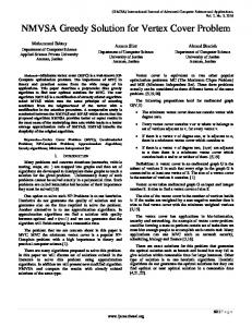
Given a planar embedding of a planar graph G = (V, E), the level of a vertex is defined as follows (see for instance [4]): the vertices on the exterior face are at level 1. Given vertices at level i, let f be an interior face of the subgraph induced by vertices at level i. If Gf denotes the subgraph induced by vertices included in f , then the vertices on the exterior face of Gf are at level i + 1. The set of vertices at level i is called the layer Li .

u2

v2

w1

x1

G f2 u1

Gf1

u3

G f3

t

v1

w2 x3

x2 u4

x4

x5

Fig. 1. Level of a planar graph

This is illustrated on Figure 1. The dashed ellipse represents an interior face on level i − 1. Depicted vertices are at level i. There are 3 interior faces (constituted respectively by the ui ’s, by {v1 , v2 , t} and {t, w1 , w2 }). Baker gave in [4] a polynomial time approximation scheme for several problems including vertex cover in planar graphs. The underlying idea is to consider k-outerplanar subgraphs of G constituted by k consecutive layers. The polynomiality of vertex cover in k-outerplanar graphs (for a fixed k) allows to achieve a (k + 1)/k approximation ratio. We adapt this technique in order to achieve an approximation scheme for MinCVC (MinCVC is NP-hard in planar graphs, see [10]). First of all, note that k-outerplanar graphs have treewidth bounded above by 3k − 1, [6]. Since MinCVC is polynomially solvable for graphs with bounded treewidth, [17], MinCVC is polynomial for k-outerplanar graphs. Theorem 4. MinCVC admits an approximation scheme in planar graphs. Proof. Given an embedding of a planar (connected) graph G, we define, as previously, the layers L1 , · · · , Lq of G. For each layer Li , we define Fi as the set of vertices of Li that are in an interior face of Li . For instance, in Figure 1, all vertices but the xi ’s are in Fi . Following the principle of the approximation scheme for vertex cover, we define an algorithm for any integer k > 0. Let Vi = Fi ∪ Li+1 ∪ Li+2 ∪ . . . ∪ Li+k , and Gi be the graph induced by Vi . Note that Gi is not necessarily connected since for example there can be several disjoint faces in Fi (there are two connected components in Figure 1). Let S ∗ be an optimum connected vertex cover on G with value opt(G), and ∗ Si = S ∗ ∩ Vi . Then of course Si∗ is a vertex cover of Gi . However, even restricted to a connected component of Gi , it is not necessarily connected. Indeed, S ∗ is connected but the path(s) connecting two vertices of S ∗ in a connected component of Gi may use vertices out of this connected component. To overcome this

problem, notice that only vertices in Fi or in Fi+k connect Vi to V \ Vi . Hence, Si∗ ∪ Fi ∪ Fi+k can be partitioned into a set of connected vertex covers on each of the connected components of Gi (since Fi and Fi+k are made of cycles). Now, take an optimum connected vertex cover on each of these connected components, and define Si as the union of these optimum solutions. Then, we have : |Si∗ ∪ Fi ∪ Fi+k | ≥ |Si |

(7)

Now, let p ∈ {1, . . . , k}. Let V0 = L1 ∪ L2 ∪ . . . ∪ Lp , G0 be the subgraph of G induced by V0 , S0∗ = S ∗ ∩ V0 , and S0 be an optimum vertex cover on G0 . With similar arguments as previously, we have: |S0∗ ∪ Fp | ≥ |S0 |

(8)

We build a solution S p on the whole graph G as follows. S p is the union of S0 and of all Si ’s for i = p mod k. Of course, S p is a vertex cover of G, since any edge of G appears in at least one Gi (or G0 ). Moreover, it is connected since: – S0 is connected, and each Si is made of connected vertex covers on the connected components of Gi ; – each of these connected vertex covers in Si is connected to Si−k (or to S0 if i = p): this is due to the fact that Fi belongs to Vi and to Vi−k (or V0 ). Hence, a level i interior face f is common to Si−k (or S0 ) and to the connected vertex cover of Si we are dealing with. Both partial solutions cover all the edges of this face f . Since f is a cycle, the two solutions are necessarily connected. In other words, each connected component of Si is connected to Si−k (or S0 ) and, by recurrence, to S0 . Consequently, the whole solution S p is connected. Summing up equation (7) for each i = p mod k and equation (8), we get: |S0∗ ∪ Fp | +

X

i=p mod k

|Si∗ ∪ Fi ∪ Fi+k | ≥ |S0 | +

X

i=p mod k

|Si |

(9)

P By definition of S p , we have |S p | ≤ |S0 | + i=p mod k |Si |. On the other hand, since only vertices in Fi (i = p mod P k) appear in two different Vi ’s (i = 0 orPi = p mod k), we get that |S0∗ ∪ Fp | + i=p mod k |Si∗ ∪ Fi ∪ Fi+k | ≤ |S ∗ | + 2 i=p mod k |Fi |. This leads to: opt(G) + 2

X

i=p mod k

|Fi | ≥ |S p |

(10)

If we consider the best solution S with value apx(G) among the S p ’s (p ∈ {1, . . . , k}), we get : opt(G) +

q 2X |Fi | ≥ apx(G) k i=1

To conclude, we observe that the following property holds:

(11)

Property 1. S ∗ takes at least one fourth of the vertices of each Fi . To see this property of S ∗ ∩ Fi , consider Fi and the set Ei of edges of G that belong to one and only one interior face of Fi (for example, in Figure 1, if there were edges {u2 , u4 } and {u3 , v1 }, they would not be in Ei ). Let ni be the number of vertices in Fi , and mi the number of edges in Ei . This graph is a collection of edge-disjoint (but not vertex-disjoint, as one can see in Figure 1) interior faces (cycles). Of course, S ∗ ∩ Fi is a vertex cover of this graph. Since this graph is a collection of interior faces (cycles), on each of these faces f S ∗ ∩ Fi cannot reject more than |f |/2 vertices. In all, |S ∗ ∩ Fi | ≥ ni −

X |f | 2

(12)

f ∈Fi

P But since faces are edge-disjoint, f ∈Fi |f | = mi . On the other hand, if Nf denotes the number of interior faces in Fi , since each face contains at least 3 P vertices, mi = f ∈Fi |f | ≥ 3Nf . Since the graph is planar, using Euler formula we get 1 + mi = ni + Nf ≤ ni + mi /3. Hence, mi ≤ 3ni /2. Finally, |S ∗ ∩ Fi | ≥ ni − mi /2 ≥ ni /4. Based on this property, we get:



8 opt(G) 1 + k



≥ apx(G)

(13)

Taking k sufficiently large leads to a 1 + ε approximation. The polynomiality of this algorithm follows from the fact that each subgraph we deal with is (at most) k + 1-outerplanar, hence for a fixed k we can find an optimum solution in polynomial time.

References 1. P. Alimonti and V. Kann. Some APX-completeness results for cubic graphs. Theor. Comput. Sci., 237(1-2):123–134, 2000. 2. E. M. Arkin, M. M. Halld´ orsson, and R. Hassin. Approximating the tree and tour covers of a graph. Inf. Process. Lett., 47(6):275–282, 1993. 3. G. Ausiello, P. Crescenzi, G. Gambosi, V. Kann, A. Marchetti-Spaccamela, and M. Protasi. Complexity and Approximation (Combinatorial Optimization Problems and Their Approximability Properties). Springer, Berlin, 1999. 4. B. S. Baker. Approximation algorithms for NP-complete problems on planar graphs. J. ACM, 41(1):153–180, 1994. 5. R. Bar-Yehuda and S. Even. On approximating a vertex cover for planar graphs. In STOC, pages 303–309, 1982. 6. H. L. Bodlaender. A partial -arboretum of graphs with bounded treewidth. Theor. Comput. Sci., 209(1-2):1–45, 1998. 7. A. Brandstadt, V. B. Le, and J. Spinrad. Graph classes : a survey. Philadelphia : Society for Industrial and Applied Mathematic, 1999.

8. H. Fernau and D. Manlove. Vertex and edge covers with clustering properties: Complexity and algorithms. In Algorithms and Complexity in Durham, pages 69– 84, 2006. 9. T. Fujito. How to trim an mst: A 2-approximation algorithm for minimum cost tree cover. In ICALP (1), pages 431–442, 2006. 10. M. R. Garey and D. S. Johnson. The rectilinear steiner tree problem in NP complete. SIAM Journal of Applied Mathematics, 32:826–834, 1977. 11. M. R. Garey and D. S. Johnson. Computer and Intractability: A Guide to the Theory of NP-Completeness. W. H. Freeman, 1979. 12. J. Guo, R. Niedermeier, and S. Wernicke. Parameterized complexity of generalized vertex cover problems. In WADS, pages 36–48, 2005. 13. S. Khot and O. Regev. Vertex cover might be hard to approximate to within 2 − ε. In IEEE Conference on Computational Complexity, pages 379–386, 2003. 14. J. K¨ onemann, G. Konjevod, O. Parekh, and A. Sinha. Improved approximations for tour and tree covers. Algorithmica, 38(3):441–449, 2003. 15. D. M¨ olle, S. Richter, and P. Rossmanith. Enumerate and expand: Improved algorithms for connected vertex cover and tree cover. In CSR, pages 270–280, 2006. 16. D. M¨ olle, S. Richter, and P. Rossmanith. Enumerate and expand: New runtime bounds for vertex cover variants. In COCOON, pages 265–273, 2006. 17. H. Moser. Exact algorithms for generalizations of vertex cover. Master’s thesis, Institut f¨ ur Informatik, Friedrich-Schiller-Universit¨ at Jena, 2005. 18. C. D. Savage. Depth-first search and the vertex cover problem. Inf. Process. Lett., 14(5):233–237, 1982. 19. S. Ueno, Y. Kajitani, and S. Gotoh. On the nonseparating independent set problem and feedback set problem for graphs with no vertex degree exceeding three. Discrete Mathematics, 72:355–360, 1988. 20. T. Wanatabe, S. Kajita, and K. Onaga. Vertex covers and connected vertex covers in 3-connected graphs. In IEEE International Sympoisum on Circuits and Systems, pages 1017–1020, 1991.