May 12, 2017 - In the Parallel Task Scheduling problem, we have given m machines and a set of jobs J. Each job j â J has a processing time p(j) â N and a ...
Complexity and Inapproximability Results for Parallel Task Scheduling and Strip Packing∗
arXiv:1705.04587v1 [cs.CC] 12 May 2017
S¨oren Henning, Klaus Jansen, Malin Rau, Lars Schmarje Institut f¨ ur Informatik, Christian-Albrechts-Universit¨at zu Kiel, Germany {stu114708,kj,mra,stu115194}@informatik.uni-kiel.de May 15, 2017
Abstract We study the Parallel Task Scheduling problem P m|sizej |Cmax with a constant number of machines. This problem is known to be strongly NP-complete for each m ≥ 5, while it is solvable in pseudo-polynomial time for each m ≤ 3. We give a positive answer to the long-standing open question whether this problem is strongly N P -complete for m = 4. As a second result, we improve the lower bound of 12 for approximating pseudo-polynomial Strip 11 Packing to 54 . Since the best known approximation algorithm for this problem has a ratio of 4 + ε, this result narrows the gap between approximation ratio and inapproximability result 3 by a significant step. Both results are proven by a reduction from the strongly N P -complete problem 3-Partition.
1
Introduction
In the Parallel Task Scheduling problem, we have given m machines and a set of jobs J. Each job j ∈ J has a processing time p(j) ∈ N and a number of required machines q(j) ∈ N. A schedule σ is a combination of two functions σ : J → N and ρ : J → {M |M ⊆ {1, . . . , m}}. The function σ maps each job to a start point in the schedule, while ρ maps each job to the set of machines it is processed on. A schedule is feasible if each machine processes at most one job at the time and each job is processed on the required number of machines. The objective is to find a feasible schedule σ minimising the makespan T := maxi∈J σ(i) + p(i). This problem is denoted with P |sizej |Cmax . If the number of machines is constant we write P m|sizej |Cmax . For a given job j ∈ J P we define its work as w(j) := p(j) · q(j). For a subset J ′ ⊆ J we define its total work as w(J ′ ) := j∈J ′ w(j). In the Strip Packing problem we have given a strip with a width W ∈ N and infinite height as well as a set of rectangular items I. Each item i ∈ I has a width wi ∈ N≤W and a height hi ∈ N. The objective is to find a feasible packing of the items I into the strip, which minimizes the packing height. A packing of the items I into the strip is a function ρ : I → Q0 × Q0 , which assigns the left bottom corner of an item to a position in the strip, such that for each item i ∈ I with ρ(i) = (xi , yi ) we have xi + wi ≤ W . An inner point of i is a point from the set inn(i) := {(x, y) ∈ R × R|xi < x < xi + wi , yi < y < yi + hi }. We say two items i, j ∈ I overlap if they share an inner point (i.e if inn(i) ∩ inn(j) 6= ∅). A packing is feasible if no two items overlap. The height of a packing is defined as H := maxi∈I yi + hi . A well known and interesting fact is that, in this setting, we can transform feasible packings to packings where all positions are integral, without enlarging the packing height [5]. This can be done by shifting all items downwards until they touch the upper border of an item or the bottom of the strip. Now all y-coordinates of the items are integral since each is given by the sum of some item heights, which are integral. The same can be done for the x-coordinate by shifting all items to the left as far as possible. Therefore we can assume that we have packings of the form ρ : I → N0 × N0 . ∗ This
work was partially supported by German Research Foundation (DFG) project JA 612 /14-2.
1
Strip packing is closely related to Parallel Task Scheduling. If we demand that jobs from the Parallel Task Scheduling are processed on contiguous machines, the resulting problem is equivalent to the Strip Packing problem. Although these problems are closely related, there are some instances that have a smaller optimal value on non-contiguous machines than on contiguous machines [30]. Related Work Parallel Task Scheduling: In 1989 Du and Leung [9] proved the problem P m|sizej |Cmax to be strongly N P -complete for all m ≥ 5, while P m|sizej |Cmax is solvable by a pseudo-polynomial algorithm for all m ≤ 3. Amoura et al. [2], as well as Jansen and Porkolab [18], presented a polynomial time approximation scheme (in short PTAS) for the case that m is a constant. A PTAS is a family of algorithms that finds a solution with an approximation ratio of (1 + ε) for any given value ε > 0. If m is polynomially bounded by the number of jobs, a PTAS still exists [21]. Nevertheless, if m is arbitrarily large, the problem gets harder. By a simple reduction from the Partition problem, one can see that there is no polynomial algorithm with approximation ratio smaller than 23 . Furthermore, there is no asymptotic algorithm with approximation ratio αOPT+β, where α < 3/2 and β polynomial in n [22]. Parallel Task Scheduling with arbitrarily large m has been widely studied [12, 30, 24, 10]. The algorithm with the best known absolute approximation ratio of 32 + ε was presented by Jansen [17]. Strip Packing: The Strip Packing problem was first studied in 1980 by Baker et al. [4]. They presented an algorithm with an absolute approximation ratio of 3. This ratio was improved by a series of papers [8, 27, 26, 28, 16]. The algorithm with the best known absolute approximation ratio by Harren, Jansen, Pr¨ adel and van Stee [15] achieves a ratio of 53 + ε. By a simple reduction from the Partition problem, one can see that it is impossible to find an algorithm with better approximation ratio than 32 , unless P = N P . However, asymptotic algorithms can achieve asymptotic approximation ratios better than 32 and have been studied in various papers [8, 14, 3]. Kenyon and R´emila [23] presented an asymptotic fully polynomial approximation scheme (in short AFPTAS) with additive term O(hmax /ε2 ), where hmax is the largest occurring item height. An approximation scheme is fully polynomial if its running time is polynomial in 1/ε as well. This algorithm was simultaneously improved by Sviridenko [29] and Bougeret et al. [6] to an algorithm with an additive term of O(log(1/ε)/ε)hmax. Furthermore, at the expense of the running time, Jansen and Soils-Oba [20] presented an asymptotic PTAS with an additive term of hmax . Recently the focus shifted to pseudo-polynomial algorithms. Jansen and Th¨ ole [21] presented an pseudo-polynomial algorithm with approximation ratio of 32 + ε. Since the partition problem is solvable in pseudo-polynomial time, the lower bound of 23 for polynomial time Strip Packing can be beaten by pseudo-polynomial algorithms. The first such algorithm with a better approximation ratio than 32 was given by Nadiradze and Wiese [25]. It has an absolute approximation ratio of 7 4 5 + ε. Its approximation ratio was independently improved to 3 + ε by Galvez, Grandoni, Ingala, and Khan [11] and by Jansen and Rau [19]. All these algorithms have a polynomial running time if the width of the strip W is bounded by a polynomial in the number of items. In contrast to Parallel Task Scheduling, Strip Packing can not be approximated arbitrarily close to 1, if we allow pseudo-polynomial running time. Adamaszek, Kociumaka, Pilipczuk and Pilipczuk [1] proved this by presenting a lower bound of 12 11 . This result also implies that Strip Packing admits no quasi-polynomial time approximation scheme, unless N P ⊆ DT IM E(2polylog(n) ). Christensen, Khan, Pokutta, and Tetali [7] list 10 major open problems related to multidimensional Bin Packing. As the 10th problem they name pseudo polynomial Strip Packing and underline the importance of finding tighter pseudo-polynomial time results for lower and upper bounds. New Results In this paper, we present two hardness results. The first result answers the longstanding open question whether the problem P 4|sizej |Cmax is strongly N P -complete. Theorem 1. The Parallel Tasks Scheduling problem on 4 machines P 4|sizej |Cmax is strongly NP-complete.
2
[1]
1
12/11
open
improvement
5/4
4/3 + ε
7/5 + ε
3/2 + ε
[19],[11]
[25]
[21]
Figure 1: The upper and lower bounds for the best possible approximation for pseudo-polynomial Strip Packing achieved so far The second result concerns pseudo-polynomial Strip Packing. We manage to adapt our reduction for P 4|sizej |Cmax to Strip Packing, by transforming the optimal schedule into a packing of rectangles interpreting the makespan as the width of the strip. This adaptation leads to the following result: Theorem 2. For each ε > 0 it is NP-Hard to approximate Strip Packing with a ratio of pseudo-polynomial time. This improves the so far best lower bound of pseudo-polynomial Strip Packing achieved so far.
12 11
to
5 4.
5 4
− ε in
In Figure 1 we display the results for
Notation For a given schedule σ we define for i ∈ J and any set of jobs J ′ ⊆ J the value #i J ′ as the number of jobs in J ′ , which finish before σ(i) (e.i. #i J ′ = |{j ∈ J ′ : σ(j) + p(j) ≤ σ(i)}|). If the job is clear from the context we write #J ′ instead of #i J ′ . Furthermore, we will use a notation defined in [9] for swapping a part of the content of two machines. Let i ∈ J be a job, that ˜ and M ˜ ′ with start point σ(i). We can swap the content is processed by at least two machines M ′ ˜ ˜ of the machines M and M after time σ(i) without violating any scheduling constraint. We define ˜,M ˜ ′ ). this swapping operation as SW AP (σ(i), M Organization of this Paper In Section 2 we will prove that P 4|sizej |Cmax is strongly NPcomplete by a reduction from the strongly NP-complete Problem 3-Partition. First, we describe the jobs to construct for this reduction. Afterward, we prove: if the 3-Partition instance is a Yes-instance, then there is a schedule with a specific makespan, and if there is a schedule with this specific makespan then the 3-Partition instance has to be a Yes-instance. While the first can be seen directly, the proof of the second is more involved. Proving the second claim, we first show that it can be w.l.o.g. supposed that each machine contains a certain set of jobs. In the next step, we prove some implications on the order in which the jobs appear on the machines which finally leads to the conclusion that the 3-Partition instance has to be a Yes-instance. In Section 3 we discuss the implications for the inapproximability of pseudo-polynomial Strip Packing.
2
Hardness of Scheduling Parallel Tasks
In the following, we will prove Theorem 1 by a reduction from the 3-Partition problem.P In the 33z Partition problem we have given a list I = (ι1 , . . . , ι3z ) of 3z positive integers, such that i=1 ιi = zD and D/4 < ιi < D/2 for each 1 ≤ i ≤ 3z. The problem is P to decide whether there exists a partition of the set I = {1, . . . , 3z} into sets I1 , . . . Iz , such that i∈Ij ιi = D for each 1 ≤ j ≤ z. P3z We define SIZE(I) = i=1 log(ιi ) as the input size of the problem. 3-Partition is strongly NPcomplete [13]. Therefore, it can not be solved in pseudo-polynomial time, unless P = N P . Construction First, we will describe how we generate an instance of P 4|sizej |Cmax from a given 3-Partition instance I in polynomial time. Let I = (ι1 , . . . , ι3z ) be a 3-Partition instance P3z with i=1 ιi = zD. If D ≤ 4z(7z + 1), we scale each number with 4z(7z + 1) such that we get a new instance I ′ := (4z(7z + 1) · ι1 , . . . , 4z(7z + 1) · ι3z ). For this instance, it holds that D′ = 4z(7z + 1)D > 4z(7z + 1) and SIZE(I ′ ) ∈ poly(SIZE(I)). Furthermore, I is a Yes-instance if and only if I ′ is a Yes-instance. Therefore, we can w.l.o.g. assume that D > 4z(7z + 1).
3
D2 D3 D4 + D6 + 3zD7 D5 + D6 + 3zD7 7 8 (z + j)D + D p(i) = D3 + D5 + 4zD7 + D8 D2 + D4 + (4z − 1)D7 + D8 D5 + (3z − j)D7 − D D4 + (3z − j)D7 D3 + zD7 + D8 2 D + 2zD7 + D8
i∈A i∈B i ∈ a, i ∈ b, i = cj ∈ c, j ∈ {0, . . . , z} i∈α i∈β i = γj ∈ γ, j ∈ {1, . . . , z} i = δj ∈ δ, j ∈ {1, . . . , z} i = λ1 i = λ2
Figure 2: Overview of the structure jobs In the following, we describe the jobs constructed for the reduction; see Figure 2 for an overview. We generate two sets A and B of 3-processor jobs. A contains z + 1 jobs with processing time pA := D2 and B contains z + 1 jobs with processing time pB := D3 . Furthermore, we generate three sets a, b and c of 2-processor jobs, such that a contains z jobs with processing time pa := D4 + D6 + 3zD7 , b contains z jobs with processing time pb := D5 + D6 + 3zD7 while c contains one job cj for each 0 ≤ j ≤ z, having processing time (z + j)D7 + D8 resulting in z + 1 jobs total in c. Last we define five sets α, β, γ, δ, and λ of 1-processor jobs, such that α contains z jobs with processing time pα := D3 + D5 + 4zD7 + D8 , β contains z jobs with processing time pβ := D2 + D4 + (4z − 1)D7 + D8 , γ contains for each 1 ≤ j ≤ z one job γj with processing time D5 + (3z − j)D7 − D resulting in |γ| = z, δ contains for each 1 ≤ j ≤ z one job δj with processing time D4 + (3z − i)D7 resulting in |δ| = z, and λ contains two jobs λ1 and λ2 with processing times p(λ1 ) := D3 + zD7 + D8 and p(λ2 ) := B + c0 = D2 + 2zD7 + D8 . We call these jobs structure jobs. Additionally, we generate for each i ∈ {1, . . . , 3z} one 1-processor job, called partition job, with processing time ιi . We name the set of partition jobs P . Last, we define W := (z + 1)(D2 + D3 + D8 ) + z(D4 + D5 + D6 ) + z(7z + 1)D7 . Note that the work of the generated jobs adds up to 4W . If we add the processing times of all generated jobs, the largest coefficient before a Di is at most 4z(7z + 1). Since 4z(7z + 1) < D, it can never happen that in the total processing time of a set of jobs the value Di , together with its coefficient, influences the coefficient of Di+1 . Furthermore, if the processing times of a set of jobs add up to a value where one of the coefficients is larger than the coefficients in W , it is not possible that in a schedule with no idle time one of the machines contains this set. In the following sections, we will prove that there is a schedule with makespan W if and only if the 3-Partition instance is a Yes-instance. Partition to Schedule Let I be a Yes-instance with partition I1 , . . . , Iz . One can easily verify that the structure jobs can be scheduled as shown in Figure 3. After each job γj , for each 1 ≤ j ≤ z, we have a gap with processing time D. We schedule the partition jobs with indices out of Ij directly after γj . Their processing times add up to D, and therefore they fit into the gap. The resulting schedule has a makespan of W . Schedule to Partition In this section, we will show that if there is a schedule with makespan W , then I is a Yes-instance. Let a schedule S with makespan W be given. We will now step by step describe why I has to be a Yes-instance. In the first step, we will show that we can transform the schedule, such that certain machines contain certain jobs. Lemma 1. We can transform the schedule S into a schedule, where M1 contains the jobs A ∪ a ∪ ˇ M3 contains the jobs A ∪ B ∪ c ∪ a α ∪ λ1 , M2 contains the jobs A ∪ B ∪ c ∪ a ˇ ∪ ˇb ∪ γˇ ∪ δ, ˆ ∪ ˆb ∪ γˆ ∪ δˆ 4
λ1
...
a1
b1 γ1
c1
δ2 A1
α1
βz−1 cz−2
β2 B1
δz−1 az−1
bz−1 γz−1
αz−1
b2 α2
βz cz−1
...
γ2
a2
Az−1
A0
Az−2
c0
δ1
Bz−1
β1 B0
Bz−2
M4 M3 M2 M1
δz az
bz
λ2 Bz
γz
cz
Az
αz
Figure 3: An optimal schedule, for a Yes-instance for ai ∈ a, bi ∈ b, Aj ∈ A, Bj ∈ B, αi ∈ α and βi ∈ β. and M4 contains the jobs B ∪ b ∪ β ∪ λ2 , with a ˇ ⊆ a, a ˆ =a\a ˇ, ˇb ⊆ b, ˆb = b \ ˇb, γˇ ⊆ γ, γˆ = γ \ γˇ , ˇ ˆ ˇ and δ ⊆ δ, δ = δ \ δ. Furthermore, if the jobs are scheduled in this way, it holds that |ˇ a| = |ˇ γ | and ˇ |ˇb| = |δ|. Proof. First, we will show that the content of the machines can be swapped without enlarging the makespan, such that M2 and M3 each contain all the jobs in A ∪ B. Let x ∈ A ∪ B be the job with the smallest starting point in this set. We can swap the complete content of the machines such that M2 and M3 contain x. Let us suppose that, after some swapping operations, M2 and ˜ ∈ {M1 , M4 } be the third machine containing the i-th M3 contain the first i jobs in A ∪ B. Let M ′ ˜ ˜ ′ ∈ {M2 , M3 }, we job xi ∈ A ∪ B. Let M be the machine not containing the (i + 1)-th job. If M transform the schedule such that M2 and M3 contain it, by performing one more swapping operation ˜,M ˜ ′ ). Therefore, we can transform the given schedule without increasing its SW AP (σ(xi ), M makespan such that M2 and M3 each contain all the jobs in A ∪ B. In the next step, we will determine the set of jobs contained by the machines M1 and M4 . The machines M2 and M3 contain besides the jobs in A ∪ B jobs with total processing time of zD4 + zD5 + zD6 + z(7z + 1)D7 + (z + 1)D8 . Hence, M2 or M3 can not contain jobs in α ∪ β ∪ λ, since their processing times contain D2 or D3 . Therefore, each job in A ∪ B ∪ α ∪ β ∪ λ is either processed on M1 or on M4 . In addition to these jobs, M1 and M4 contain further jobs with a total processing time of zD4 + zD5 + 2zD6 + 6z 2 D7 total. The only jobs with a processing time containing D6 are the jobs in the set a ∪ b. Therefore, each machine processes z jobs from the set a ∪ b. Hence, a total processing time of 3z 2 D7 is used by jobs in the set a ∪ b on each machine. This leaves a processing time of (4z 2 + z)D7 for the jobs in α ∪β ∪λ on M1 and M4 corresponding to D7 . All the 2(z + 1) jobs in α ∪ β ∪ λ contain D8 in their processing time. Therefore, each machine M1 and M4 processes z + 1 of them. We will swap the content of M1 and M4 such that λ1 is scheduled on M1 . As a consequence, M1 processes z jobs from the set α ∪ β ∪ {λ2 }, with processing times, which sum up to 4z 2 D7 in the D7 component. The jobs in α have with 4zD7 the largest amount of D7 in their processing time. Therefore, M1 processes all of them since z · 4zD7 = 4z 2 D7 , while M4 contains the jobs in β ∪ {λ2 }. Since we have p(α ∪ {λ1 }) = (z + 1)D3 + zD5 + z(4z + 1)D7 (z + 1)D8 , jobs from the set A ∪ B ∪ a ∪ b with total processing time of (z + 1)D2 + zD4 + zD6 + 3z 2D7 have to be scheduled on M1 . In this set, the jobs in A are the only jobs with processing times containing D2 , while the jobs in a are the only jobs with a processing time containing D4 . As a consequence, M1 processes the jobs A ∪ a ∪ α ∪ {λ1 }. Analogously we can deduce that M4 processes the jobs B ∪ b ∪ β ∪ {λ2 }. In the last step, we will determine which jobs are scheduled on M2 and M3 . As shown before, each of them contains the jobs A ∪ B. Furthermore, since no job in c is scheduled on M1 or M4 , and they require two machines to be processed, machines M2 and M3 both contain the set c. Additionally, each job in γ ∪ δ has to be scheduled on M2 or M3 since they are not scheduled on M1 or M4 . Each job in a ∪ b occupies one of the machines M1 and M4 . The second machine they occupy is either M2 or M3 . Let a ˇ ⊆ a be the set of jobs, which is scheduled on M2 and ˆ δ, ˇ γˆ, and a ˆ ⊆ a be the set which is scheduled on M3 . Clearly a ˇ = a\a ˆ. We define the sets ˆb, ˇb, δ, ˇ ˇ γˇ analogously. By this definition, M2 contains the jobs A ∪ B ∪ a ˇ ∪ b ∪ δ ∪ γˇ ∪ c and M3 contains 5
x2 x3 x4 x5 x6 x8
M1 #i A #i α + #i {λ1 } #i a #i α #i a #i α + #i {λ1 }
M2 #i A #i B #i a ˇ + #i δˇ ˇ #i b + #i γˇ #i a ˇ + #iˇb #i c
M3 #A #i B #i a ˆ + #i δˆ ˆ #i b + #i γˆ #i a ˆ + #iˆb #i c
M4 #i β + #i {λ2 } #i B #i β #i b #i b #i β + #i {λ2 }
Table 1: Overview of the values of the coefficients at the start point of a job i, if i is scheduled on machine Mj . the jobs A ∪ B ∪ a ˆ ∪ ˆb ∪ δˆ ∪ γˆ ∪ c. ˇ First, we notice that |ˇ We still have to show that |ˇ a| = |ˇ γ | and |ˇb| = |δ|. a| + |ˇb| = z since these 6 jobs are the only jobs with a processing time containing D . So besides the jobsP in A ∪ B ∪ c ∪ a ˇ ∪ ˇb, z 4 5 ˇ M2 contains jobs time of (z − |ˇ a|)D + (z − |b|)D + i=1 (3z − i)D7 = Pzwith total processing 4 5 7 ˇ |b|D + |ˇ a|D + i=1 (3z − i)D . Since the jobs in δ are the only jobs in δ ∪ γ having a processing ˇ = |ˇb| and analogously |ˇ time containing D4 , we have |δ| γ | = |ˇ a|. In the next steps, we will prove that it is possible to transform the order in which the jobs appear on the machines to the order in Figure 3. Notice that, since there is no idle time in the schedule, each start point of a job i is given by the sum of processing times of the jobs on the same machine scheduled before i. So the start position σ(i) of a job i has the form σ(i) = x0 + x2 D2 + x3 D3 + x4 D4 + x5 D5 + x6 D6 + x7 D7 + x8 D9 for −zD ≤ x0 ≤ zD and 0 ≤ xj ≤ 4z(7z + 1) ≤ D for each 2 ≤ j ≤ 8. This allows us to make implications about the correlation between the number of jobs scheduled on different machines when a job from the set A ∪ B ∪ a ∪ b ∪ c starts. For example, let us look at the coefficient x2 . This value is just influenced by jobs with processing times containing D2 . The only jobs with these processing times are the jobs in the set A ∪ β ∪ {λ2 }. The jobs in β ∪ {λ2 } are just processed on M4 , while the jobs in A each are processed on the three machines M1 , M2 , and M3 . Therefore, we know that at the starting point σ(i) of a job i scheduled on machines M1 , M2 or M3 we have that x2 = #i A. Furthermore, if i is scheduled on M4 we know that x2 = #i β + #i {λ2 }. In Table 1 we present which sets influences which coefficients in which way when job i is started on the corresponding machine. Let us consider the start point σ(i) of a job i, which uses more than one machine. We know that σ(i) is the same on all the used machines and therefore the coefficients are the same as well. In the following, we will study for each of the sets A, B, a, b, c what we can conclude for the starting times of these jobs. For each of the sets, we will present an equation, which holds at the start of each item in this set. These equations give us a strong set of tools for our further arguing. First, we will consider the start points of the jobs in A. Each job A′ ∈ A is scheduled on machines M1 , M2 and M3 . Therefore, we know that at s(A′ ) we have #A′ B =x3 #A′ α + #A′ {λ1 } =x8 #A′ c. ˆ ˇ + #A′ a ˆ + #A′ ˆb. Since #A′ a = #A′ a ˇ + #A′ ˇb = #A′ a Furthermore, we know that #A′ a =x6 #A′ a ˆ ˇ and #A′ b = #A′ b + #A′ b, we can deduce that #A′ a = #A′ b. Additionally, we know that #A′ α =x5 γ . Thanks to this equality, we can show that #A′ α = #A′ b. First, we show #ˇb + #ˇ γ =x5 #ˆb + #ˆ #A′ α ≥ #A′ b. Let b′ ∈ b be the last job in b scheduled before A′ if there is any. Let us w.l.o.g assume that b ∈ ˆb. It holds that #A′ b = #b′ b + 1 =x5 #b′ ˆb + #b′ γˆ + 1 ≤ #A′ ˆb + #A′ γˆ =x5 #A′ α. If there is no such b′ we have #A′ b = 0 ≤ #A′ α. Next, we show #A′ α ≤ #A′ b. Let b′′ ∈ A be the first job in b scheduled after A if there is any. Let us w.l.o.g assume that b ∈ ˇb. It holds that #A′ b = #b′′ b =x5 #b′′ ˇb + #b′′ γˇ ≥ #A′ ˇb + #A′ γˇ =x5 #A′ α. If there is no such b′′ , we have #A′ b = z ≥ #A′ α. As a consequence we have #A′ α = #A′ b. In summary, we can deduce that #A′ c − #A′ {λ1 } = #A′ B − #A′ {λ1 } = #A′ α = #A′ b = #A′ a.
(1)
Analogously, we can deduce that at the start of each B ′ ∈ B we have that #B ′ c − #B ′ {λ2 } = #B ′ A − #B ′ {λ2 } = #B ′ β = #B ′ a = #B ′ b. 6
(2)
Each item a′ ∈ a is scheduled on machine M1 and on one of the machines M2 or M3 . For each possibility, we can deduce the equation #a′ B =x3 #a′ α + #a′ {λ1 } =x8 #a′ c.
(3)
Analogously, we deduce for each b′ ∈ b that #b′ A =x2 #b′ β + #b′ {λ2 } =x8 #b′ c.
(4)
Last, each item c′ ∈ c is scheduled on M2 and M3 . Let a′ ∈ a be the job with the smallest ˆ + #c′ ˆb ≤ σ(a′ ) ≥ σ(c′ ). Let us w.l.o.g assume that a′ ∈ a ˆ. It holds that #c′ a ˇ + #c′ ˇb =x6 #c′ a ˆ ˆ ˇ. As a consequence, we have #c′ ˇb ≤ #c′ a ˆ + #c′ a ˇ = #c′ a ˆ + #a′ a ˆ + #a′ b =x6 #a′ a = #a′ a #a′ a ′ ˇ. Analogously, let b ∈ b be the job with the smallest σ(b′ ) ≥ σ(c′ ). Let us and #c′ ˆb ≤ #c′ a ˇ + #b′ ˇb =x6 #b′ b = ˇ + #c′ ˇb ≤ #b′ a ˆ + #c′ ˆb =x6 #c′ a w.l.o.g assume that b′ ∈ ˇb. It holds that #c′ a ˇ ˆ ˇ ˆ ˆ ˆ ≤ #c′ b. As a consequence, we can ˇ ≤ #c′ b and #c′ a ˇ = #c′ b + #c′ b. Therefore, #c′ a #b′ b + #b′ a deduce that (5) #c′ b = #c′ a These equations give us the tools to analyze the given schedule with makespan W . First, we will show that in this schedule the first and last jobs have to be elements from the set A∪B, (see Lemma 2). After that, we will prove that the jobs in A and jobs in B have to be scheduled alternating, (see Lemma 3). With the knowledge gathered in the proofs of Lemma 2 and Lemma 3, we can prove that the given schedule can be transformed such that all jobs are scheduled continuously, and that I has to be a Yes-instance (see Lemma 3). Lemma 2. The first and the last job on M2 and M3 are elements of A ∪ B. Proof. Let i := arg mini∈A∪B si be the job with the smallest start point in A ∪ B, (i.e. #i A = 0 = #i B). We have to consider each case i ∈ A and i ∈ B and to show that its starting time has the value si = 0. If i ∈ A it holds that 0 = #i B =(1) #i α + #i {λ1 } =(1) #i a + #i {λ1 } and therefore #i a = #i α = 0 = #i {λ1 }. The jobs a ∪ α ∪ {λ1 } ∪ A are the only jobs, which are contained on machine M1 . Since #i A = 0 as well, it has to be that si = 0 and therefore i is the first job on M2 and M3 . If i ∈ B it holds that 0 = #i A =(2) #i β + #i {λ2 } =(2) #i b + #i {λ2 } and therefore #i b = #i β = 0 = #i {λ2 }. The jobs b ∪ β ∪ {λ2 } ∪ B are the only jobs, which are contained on machine M4 . Since #i B = 0 as well, it has to be that si = 0 and therefore i is the first job on M2 and M3 . We have shown that the first job on M2 and M3 hast to be a job from the set A ∪ B. Since the schedule stays valid, if we mirror the schedule such that the new start points are s′ (i) = W − s(i) − p(i) for each job i, the last job has to be in the set A ∪ B as well. Next, we will show that the items in the sets A and B have to be scheduled alternating. Let (A0 , . . . , Az ) be the set A and (B0 , . . . , Bz ) be the set B each ordered by increasing size of the starting points. Lemma 3. If the first item on M2 is the job B0 ∈ B it holds for each item i ∈ {0, . . . , z} that #Ai B − #Ai {λ1 } = #Ai A
(6)
with #Ai {λ1 } = 1. Proof. We will prove this claim inductively and per contradiction. Assume #A0 B − #A0 {λ1 } > #A0 A = 0. Therefore, we have 1 ≤ #A0 B − #A0 {λ1 }. Let a′ ∈ a, b′ ∈ b and c′ ∈ c be the first started jobs in their sets. Since #A0 b =(1) #A0 a =(1) #A0 c − #A0 {λ1 } =(1) #A0 B − #A0 {λ1 } ≥ 1, the jobs a′ , b′ and c′ start before A0 . It holds that #b′ c =(4) #b′ A = 0. Therefore, c′ has to start after b′ resulting in #c′ b ≥ 1. Furthermore, we have #a′ c =(3) #a′ B ≥ 1. Hence, c′ has to start before a′ resulting in #c′ a = 0. In total we have 1 ≤ #c′ b =(5) #c′ a = 0 contradicting the assumption #A0 B − #A0 {λ1 } > #A0 A = 0. Therefore, we have #A0 B −#A0 {λ1 } ≤ #A0 A = 0. As a consequence, it holds that 1 ≤ #A0 B ≤ #A0 {λ1 } ≤ 1 and we can conclude #A0 B = 1 = #A0 {λ1 } as well as #A0 B − #A0 {λ1 } = #A0 A. 7
Choose i ∈ {0, . . . , z} such that #Ai′ B − #Ai′ {λ1 } = #Ai′ A for all i′ ∈ {0, . . . i}. As a consequence, we have #Bi B = i = #Ai A = #Ai B − 1. Therefore Bi has to be scheduled before Ai . Additionally, we have #Bi B − 1 = #Bi−1 B = i − 1 = #Ai−1 A = #Ai−1 B − 1, so Bi has to be scheduled after Ai−1 . Therefore, we have #Bi B = #Bi A and as a consequence i = #Bi B = #Bi A = #B ′ c = #B ′ β + #B ′ {λ2 } = #B ′ a + #B ′ {λ2 } = #B ′ b + #B ′ {λ2 }.
(7)
We will now prove our claim for Ai+1 . Claim. #Ai+1 B − #Ai+1 {λ1 } ≤ #Ai+1 A Assume for contradiction that #Ai+1 B − #Ai+1 {λ1 } > #Ai+1 A. As a consequence, we have #Ai+1 B − #Ai+1 {λ1 } − #Ai B + #Ai {λ1 } ≥ 2. Therefore, there are jobs Bi+1 , Bi+2 ∈ B, a′ , a′′ ∈ a, b′ , b′′ ∈ b and c′ , c′′ ∈ c, that are scheduled between Ai and Ai+1 since equality (1) holds. Let us suppose that σ(a′ ) ≤ σ(a′′ ), σ(b′ ) ≤ σ(b′′ ) and σ(c′ ) ≤ σ(c′′ ). Next, we will deduce in which order the jobs a′ , a′′ , b′ , b′′ , c′ , c′′ , Bi+1 , and Bi+2 appear in the schedule. It holds that #b′′ c =(4) #b′′ A = #Ai A + 1 = #Ai B =(1) = #Ai c. Therefore, b′ and b′′ have to start before c′ . Furthermore we have #c′ a =(5) #c′ b ≥ #Ai b + 2 =(1) #Ai a + 2. Hence, a′′ hast to start before c′ as well. Additionally, it holds that #Bi+2 c =(2) #Bi+2 A = #Ai A + 1 = #Ai B =(1) #Ai c. As a consequence, Bi+2 has to start before c′ . Additionally, a′′ has to start before Bi+1 , since #a′′ B =(3) #a′′ c = #Ai c =(1) #Ai B. To this point, we have deduced that the jobs have to appear in the following order in the schedule: Ai , a′ , a′′ , Bi+1 , Bi+2 , c′ , c′′ , Ai+1 . This schedule is not feasible, since we have #Ai a+2 ≤S #Bi+1 a≤(2) #Bi+1 A =S #Ai A + 1=(1) #Ai a + 1, a contradiction to the assumption #Ai+1 B − #Ai+1 {λ1 } > #Ai+1 A. Therefore, it holds that #Ai+1 B − #Ai+1 {λ1 } ≤ #Ai+1 A Claim. #Ai+1 B − #Ai+1 {λ1 } ≥ #Ai+1 A Assume for contradiction that #Ai+1 B−#Ai+1 {λ1 } < #Ai+1 A. It follows that #Ai+1 B = #Ai B since #Ai B − #Ai {λ1 } ≤ #Ai+1 B − #Ai+1 {λ1 } ≤ #Ai+1 A − 1 = #Ai A = #Ai B − #Ai {λ1 }. Furthermore, there has to be at least one job Bi+1 ∈ B that starts after Ai+1 since |A| = |B|. Therefore, we have #Bi+1 c − #Bi c = #Bi+1 A − #Bi A ≥ 2. As a consequence, there are jobs c′ , c′′ ∈ c which are scheduled between Bi and Bi+1 . Let c′ be the first job in c scheduled after Bi ans c′′ be the next. Since we do not know the value of #Bi {λ2 } or #Bi+1 {λ2 }, we can just deduce from equation (2) that #Bi+1 a − #Bi a ≥ 1. Therefore, there has to be a job a′ ∈ a that is scheduled between Bi and Bi+1 . We will now look at the order in which the jobs Ai , Ai+1 , c′ , c′′ and a′ have to be scheduled. First, we know that Ai and Ai+1 have to be scheduled between c′ and c′′ , since #Ai c =(1) #Ai B =S #Bi B + 1 =(7) #Bi A+ 1 =(2) #Bi c+ 1 and #Ai+1 c =(1) #Ai+1 B =S #Bi B + 1 =(7) #Bi A+ 1 =(2) #Bi c + 1. Furthermore, we know that a′ has to be scheduled between c′ and c′′ as well, since #a′ c =(3) #a′ B =S #Bi B + 1 =(7) #Bi A + 1 =(2) #Bi c + 1. As a consequence, we can deduce that there is a job b′ ∈ b which is scheduled between c′ and c′′ , since #c′′ b =(5) #c′′ a ≥S #c′ a + 1 =(5) #c′ b + 1. We know about this b′ that #b′ A =(4) #b′ c =S #Bi c + 1 =(2) #Bi A + 1, so b′ has to be scheduled between Ai and Ai+1 . In summary, the jobs are scheduled as follows: Bi , c′ , Ai , b′ , Ai+1 , c′′ , Bi+1 . However, this schedule is infeasible since #Ai b =(1) #Ai B − #Ai {λ1 } =S #Ai+1 B − #Ai+1 {λ1 } =(1) #Ai+1 b =S #Ai b + 1. This contradicts the assumption #Ai+1 B − #Ai+1 {λ1 } < #Ai+1 A. Altogether, we have shown that #Ai+1 B − #Ai+1 {λ1 } = #Ai+1 A. A direct consequence of Lemma 3 is that the last job on M2 is a job in A. Since the equations (1) and (2), as well as (3) and (4), are symmetric, we can deduce an analogue statement if the first job on M2 is in A. More precisely in this case we can show that #i A − #i {λ2 } = #i B and #i {λ2 } = 1 for each i ∈ B. This would imply that the last job on M2 is a job in B. Since we can mirror the schedule such that the last job is the first job, we can suppose that the first job on M2 is a job out of B. In this case a further direct consequence of Lemma 3 and equation (1) is the equation (8) i = #Ai A = #Ai B − 1 = #Ai c − 1 = #Ai α = #Ai b = #Ai a
8
Lemma 4. I is a Yes-instance and we can transform the schedule such that all jobs are scheduled on continuous machines. Proof. First, we will show that λ2 is scheduled after the last job in B. Assume there is an i ∈ {0, . . . , z} with #Bi {λ2 } > 0. Let i be the smallest of these indices. We know that i − 1 =(7) #Bi A − 1 = #Bi A − #Bi {λ2 } =(2) #Bi a. Since #Ai b =(1) #Ai a =(8) i = #Bi a + 1 =(2) #Bi b + 1 there has to be an unique a′ ∈ a and an unique b′ ∈ b scheduled between Bi and Ai . Furthermore, since #Ai c =(8) i + 1 and #Bi c =(7) i, there has to be a c′ ∈ c scheduled between Bi and Ai as well. At the start of b′ it holds that #b′ c =(4) #b′ A = #Ai−1 A + 1 =(1) #Ai−1 c, so b′ has to start before c′ . Additionally, at the start of a′ we have #a′ c =(4) #a′ B = #Bi B + 1 =(7) #Bi c + 1 and therefore a′ hast to start after c′ . In total, the jobs appear in the following order: Bi , b′ , c′ , a′ , Ai . But this can not be the case, since we have #Bi−1 a =S #c′ a =(5) #c′ b =S #Bi−1 b + 1 = #Bi−1 a + 1. Hence, we have contradicted that assumption. As a consequence, we have #Bi {λ2 } = 0 for all i ∈ {0, . . . , z} and therefore #Bi b = #Bi a = #Bi c = #Bi β = #Bi A = #Bi B = i.
(9)
In the next step, we will prove that M1 processes the jobs A ∪ a ∪ α ∪ {λ1 } in the order λ1 , A0 , a1 , α1 , A1 , a2 , α2 , A2 , . . . , az , αz , Az , where ai ∈ a and αi ∈ α for each i ∈ {1, . . . z}. Equation (8) and Lemma 3 ensure that the first job on M1 is the job λ1 and the second job is A0 . For each i ∈ {1, . . . , z} it holds that #Ai α =(8) #Ai−1 α + 1 and #Ai a =(8) #Ai−1 a + 1. Therefore, there is scheduled exactly one job ai ∈ a and one job αi ∈ α between the jobs Ai−1 and Ai . It holds that #Ai−1 a + 1 =(8) i =(9) #Bi a. Therefore, ai has to be scheduled between Ai−1 and Bi . As a consequence, we have #ai α + 1 = #ai α + #ai {λ1 } =(3) #ai B = #Bi B =(9) #Bi a = #a′ a + 1. Therefore, ai has to be scheduled before αi and the jobs appear in machine M1 in the described order. As a result, we know about the start point of Ai that σ(Ai ) = p(λ1 ) + i · pa + i · pα + i · pA = D3 + zD7 + D8 + i(D4 + D6 + 3zD7 ) + i(D3 + D5 + 4zD7 + D8 ) + iD2 = iD2 + (i + 1)D3 + iD4 + iD5 + iD6 + (7zi + z)D7 + (i + 1)D8 . Now, we will show, that the machine M4 processes the jobs B ∪ b ∪ β ∪ {λ2 } in the order B0 , β1 , b1 , B1 , β2 , b2 , B2 , . . . , βz , bz , Bz , λ2 , where bi ∈ b and βi ∈ β for each i ∈ {1, . . . z}. The first job on M4 is the job B0 . Equation (9) ensures that between the jobs Bi and Bi+1 there is scheduled exactly one job bi+1 ∈ b and exactly one job βi+1 ∈ β. It holds that #Ai b + 1 =(8) i + 1 =(9) #Bi+1 b. Therefore, bi+1 has to be scheduled between Ai and Bi+1 . As a consequence, it holds that #bi+1 β = #bi+1 β + #bi+1 {λ2 } = #bi+1 A = #Bi+1 A = #Bi+1 b = #bi+1 b + 1. Hence, bi+1 has to be scheduled after βi+1 and the jobs on machine M4 appear in the described order. As a result, we know about the start point of Bi that σ(Bi ) = ipb + ipβ + ipB = iD2 + iD3 + iD4 + iD5 + iD6 + (i(7z − 1))D7 + iD8 . Next, we can deduce, that the jobs in c are scheduled as shown in Figure 3. We have #Bi c =(9) i =(8) #Ai c−1. Therefore, there exists an c′ ∈ c for each i ∈ {0, . . . , z}, which is scheduled between Bi and Ai . The processing time between Bi and Ai is exactly σ(Ai )−σ(Bi )−p(Bi ) = (z+i)D7 +D8 . As a consequence, one can see with an inductive argument that ci ∈ c with p(ci ) = (z + i)D7 + D8 has to be positioned between Bi and Ai , since the job in c with the largest processing time cz only fits between Bz and Az . In this step, we will transform the schedule, such that all jobs are scheduled on continuous machines. To this point, this property is obviously fulfilled by the jobs in A ∪ B ∪ c. However, the jobs in a ∪ b might be scheduled on nonconsecutive machines. We know that the ai and bi are scheduled between Ai−1 and Bi . One part of ai is scheduled on M1 and one part of bi is scheduled on M4 , while each second part is scheduled either on M2 or on M3 but both parts on different machines, 9
because σ(Bi )−σ(Ai−1 )−p(Ai ) = D4 +D5 +D6 +(6z−i)D7 < D4 +D5 +2D6 +6zD7 = p(ai )+p(bi ) for each i ∈ {0, . . . , z}. Since Ai and Bi+1 both are scheduled on machines M2 and M3 , we can swap the content of the machines between these jobs such that the second part of ai is scheduled on M2 and the second part of bi is scheduled on M3 . We do this swapping step for all i ∈ {0, . . . , z −1} such that all second parts of jobs in a are scheduled on M2 and all second part of jobs in b are scheduled on M3 respectively. After this swapping step, all jobs are scheduled on continuous machines. Now, we will show that I is a yes-instance. To this point we know that M2 contains the jobs A ∪ B ∪ a ∪ c. Since a ˇ = a, it has to hold by Lemma 1, using |ˇ a| = |ˇ γ |, that γˇ = γ implying that ˇ we have δˇ = ∅ and therefore M2 contains all jobs in γ. Furthermore, since ˇb = ∅ and |ˇb| = |δ|, M2 does not contain any job in δ. Besides the jobs A ∪ B ∪ a ∪ c ∪ γ, M2 processes further jobs with total processing time zD. Therefore, all the jobs in P are processed on M2 . We will now analyse where the jobs in γ are scheduled. The only possibility where these jobs can be scheduled is the time between ai and Bi for each i ∈ {1, . . . , z} since at each other time the machine is occupied by other jobs. The processing time between the end of ai and the start of Bi is exactly σ(Bi ) − σ(Ai−1 ) − p(Ai−1 ) − p(ai ) = D5 + (3z − i)D7. The job in γ with the largest processing time is the job γ1 with p(γ1 ) = D5 + (3z − 1)D7 − D. This job only fits between ai and B1 . Inductively we can show that γi ∈ γ with p(γi ) = D5 + (3z − i)D7 − D has to be scheduled between ai and Bi on M2 . Furthermore, since p(γi ) = D5 + (3z − i)D7 − D and the processing time between the end of ai and the start of Bi is D5 + (3z − i)D7 , there is exactly D processing time left. These processing time has to be occupied by the jobs in P since this schedule has no idle times. Therefore, we have for each i ∈ {1, . . . , z} a disjunct subset Pi ⊆ P containing jobs with processing times adding up to D. As a consequence I is a Yes-instance.
3
Hardness of Strip Packing
In the transformed schedule, all jobs are scheduled on contiguous machines. As a consequence, we have proven that this problem is strongly N P -complete even if we restrict the set of feasible solutions to those where all jobs are scheduled on continuous machines. We will now describe how this insight delivers a lower bound of 54 for the best possible approximation ratio for pseudopolynomial Strip Packing and in this way prove Theorem 2. To show our hardness result for Strip Packing, let us consider the following instance. We define W := (z + 1)(D2 + D3 + D8 ) + z(D4 + D5 + D6 ) + z(7z + 1)D7 as the width of the considered strip, so it is the same as the considered makespan in the scheduling problem. For each job j defined in the reduction above, we define an item i with w(i) = p(j) and height h(i) = q(j). Now, we can show analogously that if the 3-Partition instance is a Yes-instance there is a packing of height 4 (one example is the packing in Figure 3) and if there is a packing with height 4 then the 3-Partition instance has to be a Yes-instance. If the 3-Partition instance is a No-instance, the optimal packing has a height of at least 5 since the optimal height for this instance is integral. Therefore, we can not approximate Strip Packing in pseudo-polynomial time better than 45 .
4
Conclusion
In this paper, we positively answered the long standing open question whether P 4|sizej |Cmax is strongly N P -complete. Now, for each number of machines m it is known whether the problem P m|sizej |Cmax is strongly N P -complete. Furthermore, we have improved the lower bound for pseudo-polynomial Strip Packing to 45 . Since the best known algorithm has an approximation ratio of 34 , this still leaves a gap between the lower bound and the best known algorithm. With the techniques used in this paper, a lower bound of 43 for pseudo-polynomial Strip Packing can not be proven, since P 3|sizej |Cmax is solvable in pseudo-polynomial time and in the generated solutions all jobs are scheduled contiguously. Moreover, we believe that it is possible to find an algorithm with approximation ratio 45 + ε.
10
References [1] Anna Adamaszek, Tomasz Kociumaka, Marcin Pilipczuk, and Michal Pilipczuk. ness of approximation for strip packing. CoRR, abs/1610.07766, 2016. http://arxiv.org/abs/1610.07766.
HardURL:
[2] Abdel Krim Amoura, Evripidis Bampis, Claire Kenyon, and Yannis Manoussakis. Scheduling independent multiprocessor tasks. Algorithmica, 32(2):247–261, 2002. doi:10.1007/s00453-001-0076-9. [3] Brenda S. Baker, Donna J. Brown, and Howard P. Katseff. A 5/4 algorithm for two-dimensional packing. Journal of Algorithms, 2(4):348–368, 1981. doi:10.1016/0196-6774(81)90034-1. [4] Brenda S. Baker, Edward G. Coffman Jr., and Ronald L. Rivest. Orthogonal packings in two dimensions. SIAM Journal on Computing, 9(4):846–855, 1980. doi:10.1137/0209064. [5] Nikhil Bansal, Jos´e R. Correa, Claire Kenyon, and Maxim Sviridenko. Bin packing in multiple dimensions: Inapproximability results and approximation schemes. Mathematics of Operations Research, 31(1):31–49, 2006. doi:10.1287/moor.1050.0168. [6] Marin Bougeret, Pierre-Fran¸cois Dutot, Klaus Jansen, Christina Robenek, and Denis Trystram. Approximation algorithms for multiple strip packing and scheduling parallel jobs in platforms. Discrete Mathematics, Algorithms and Applications, 3(4):553–586, 2011. doi:10.1142/S1793830911001413. [7] Henrik I. Christensen, Arindam Khan, Sebastian Pokutta, and Prasad Tetali. Approximation and online algorithms for multidimensional bin packing: A survey. Computer Science Review, 2017. doi:10.1016/j.cosrev.2016.12.001. [8] Edward G. Coffman Jr., Michael R. Garey, David S. Johnson, and Robert Endre Tarjan. Performance bounds for level-oriented two-dimensional packing algorithms. SIAM Journal on Computing, 9(4):808–826, 1980. doi:10.1137/0209062. [9] Jianzhong Du and Joseph Y.-T. Leung. Complexity of scheduling parallel task systems. SIAM Journal on Discrete Mathematics, 2(4):473–487, 1989. doi:10.1137/0402042. [10] Anja Feldmann, Jir´ı Sgall, and Shang-Hua Teng. Dynamic scheduling on parallel machines. Theoretical Computer Science, 130(1):49–72, 1994. doi:10.1016/0304-3975(94)90152-X. [11] Waldo G´ alvez, Fabrizio Grandoni, Salvatore Ingala, and Arindam Khan. Improved pseudopolynomial-time approximation for strip packing. In 36th IARCS Annual Conference on Foundations of Software Technology and Theoretical Computer Science (FSTTCS), pages 9:1–9:14, 2016. doi:10.4230/LIPIcs.FSTTCS.2016.9. [12] Michael R. Garey and Ronald L. Graham. Bounds for multiprocessor scheduling with resource constraints. SIAM Journal on Computing, 4(2):187–200, 1975. doi:10.1137/0204015. [13] Michael R. Garey and David S. Johnson. Computers and Intractability: A Guide to the Theory of NP-Completeness. W. H. Freeman, 1979. [14] Igal Golan. Performance bounds for orthogonal oriented two-dimensional packing algorithms. SIAM Journal on Computing, 10(3):571–582, 1981. doi:10.1137/0210042. [15] Rolf Harren, Klaus Jansen, Lars Pr¨adel, and Rob van Stee. A (5/3 + ǫ)approximation for strip packing. Computational Geometry, 47(2):248–267, 2014. doi:10.1016/j.comgeo.2013.08.008. [16] Rolf Harren and Rob van Stee. Improved absolute approximation ratios for two-dimensional packing problems. In Approximation, Randomization, and Combinatorial Optimization. Algorithms and Techniques,, volume 5687 of Lecture Notes in Computer Science, pages 177–189. Springer, 2009. doi:10.1007/978-3-642-03685-9_14. 11
[17] Klaus Jansen. A (3/2 + ε) approximation algorithm for scheduling moldable and non-moldable parallel tasks. In 24th ACM Symposium on Parallelism in Algorithms and Architectures, (SPAA), pages 224–235, 2012. doi:10.1145/2312005.2312048. [18] Klaus Jansen and Lorant Porkolab. Linear-time approximation schemes for scheduling malleable parallel tasks. Algorithmica, 32(3):507–520, 2002. doi:10.1007/s00453-001-0085-8. [19] Klaus Jansen and Malin Rau. Improved approximation for two dimensional strip packing with polynomial bounded width. In WALCOM: Algorithms and Computation, volume 10167 of LNCS, pages 409–420, 2017. doi:10.1007/978-3-319-53925-6_32. [20] Klaus Jansen and Roberto Solis-Oba. Rectangle packing with one-dimensional resource augmentation. Discrete Optimization, 6(3):310–323, 2009. doi:10.1016/j.disopt.2009.04.001. [21] Klaus Jansen and Ralf Th¨ ole. Approximation algorithms for scheduling parallel jobs. SIAM Journal on Computing, 39(8):3571–3615, 2010. doi:10.1137/080736491. [22] Berit Johannes. Scheduling parallel jobs to minimize the makespan. Journal of Scheduling, 9(5):433–452, 2006. doi:10.1007/s10951-006-8497-6. [23] Claire Kenyon and Eric R´emila. A near-optimal solution to a two-dimensional cutting stock problem. Mathematics of Operations Research, 25(4):645–656, 2000. doi:10.1287/moor.25.4.645.12118. [24] Walter Ludwig and Prasoon Tiwari. Scheduling malleable and nonmalleable parallel tasks. In 5th Annual ACM-SIAM Symposium on Discrete Algorithms (SODA), pages 167–176, 1994. [25] Giorgi Nadiradze and Andreas Wiese. On approximating strip packing with a better ratio than 3/2. In 27th Annual ACM-SIAM Symposium on Discrete Algorithms (SODA), pages 1491–1510, 2016. doi:10.1137/1.9781611974331.ch102. [26] Ingo Schiermeyer. Reverse-fit: A 2-optimal algorithm for packing rectangles. In 2nd Annual European Symposium on Algorithms (ESA) - Algorithms, pages 290–299, 1994. doi:10.1007/BFb0049416. [27] Daniel Dominic Sleator. A 2.5 times optimal algorithm for packing in two dimensions. Information Processing Letters, 10(1):37–40, 1980. doi:10.1016/0020-0190(80)90121-0. [28] A. Steinberg. A strip-packing algorithm with absolute performance bound 2. SIAM Journal on Computing, 26(2):401–409, 1997. doi:10.1137/S0097539793255801. [29] Maxim Sviridenko. A note on the kenyon-remila strip-packing algorithm. Information Processing Letters, 112(1-2):10–12, 2012. doi:10.1016/j.ipl.2011.10.003. [30] John Turek, Joel L. Wolf, and Philip S. Yu. Approximate algorithms scheduling parallelizable tasks. In 4th annual ACM symposium on Parallel algorithms and architectures (SPAA), pages 323–332, 1992. doi:10.1145/140901.141909.
12