Component Based Performance Prediction Xiuping Wu
David McMullan
Murray Woodside
Carleton University Ottawa, Canada K1S 5B6
Carleton University Ottawa, Canada K1S 5B6
Carleton University Ottawa, Canada K1S 5B6
[email protected]
[email protected]
[email protected]
ABSTRACT Component Based Software Engineering (CBSE) exploits re-usability of configurable components to generate software products more quickly, and with higher quality. CBSE offers potential advantages for performance engineering. If most of a new system consists of existing software components, it should be possible to predict properties like performance more easily, than if all of the software is new. The performance-sensitive properties of the components can be extracted and stored in a library, and used to build a predictive model for the performance of a proposed product. This paper describes an approach based on performance submodels for each component, and a system assembly model to describe the binding together of library components and new components into a product. In this work a component can be arbitrarily complex, including a subsystem of concurrent processes. The description pays particular attention to identifying the information that must be provided with the components, and with the bindings, and to providing for parameterization to describe different configurations and workloads.
General Terms Performance
Keywords Component Based Software Engineering(CBSE), Performance prediction, Performance submodels, Assembly model
1. INTRODUCTION Research in Component Based Software Engineering has focussed on functional aspects, with relatively little reported on design for non-functional properties such as performance. One difficulty is the need to consider many potential execution environments for a system. Sherif, Yacoub et. al. [9] proposed a way to characterize a software component, in which they mention nonfunctional attributes, without details about how to describe them and use them. Sitaraman et. al. [4] argued that performance specification of software components and assemblies is a basic problem that must be solved to enable software engineers to assemble systems from components. It would be very helpful if we can build a performance model for each component and then assemble these sub-models for prediction according to the system design, especially if there are tools or methodology that can automate these processes. Our research work has been motivated by this thought.
Performance model of the Application System
Application System Product glue code Customized Component A
glue model Customized Component B select and customize
Component Library
Infrastructure support
Building the software from a Component Library
and Model
Customized Submodels
Assembly Specifications
select with parameters Library of Component Submodels
Library of Infrastructure Submodels
Building the model from a Component Submodel Library
Figure 1 Component Based System development
The development of component based software systems can be generalized [10] as shown in Figure 1. Using the same specification as for the component-based software, our approach is to assemble performance sub-models for these components into a system-level performance model, using an automated tool for model assembly.
2. COMPONENTS IN AN LQN PERFORMANCE MODEL LQN models [5] extend the traditional queuing network models by considering both software and hardware contention, and the impact of layers on service time. An LQN model is expressed as a set of objects called “tasks” offering services (like methods) called “entries”; entries of one task make requests to entries of others at lower layers. LQN has been used for many industrial case studies and has demonstrated the power of early performance prediction. For component based software system prediction or evaluation, components are expressed as a type of LQN submodel [1], and the binding definition for the overall system is expressed as another LQN, with additional information to define parameters and bindings. Within a component submodel, the parts such as tasks, entries, processors and interactions will be called its “elements”.
2.1 Concept and definition of LQN component model A component submodel represents a sub-system that can be incorporated into a software product. An example submodel for a component called an Application Server is shown in Figure 2. The controller task interprets the request, the ReportGen task creates and edits reports on an SQL database, and the ResultsCache task stores report data for reuse, to assist the assembly of complex reports and the presentation of the same data from different points of view, or at different levels of detail. The stub portion includes a processor for each software element, which allows unconstrained allocation to different processors. There is a single incoming interface, showing that all requests come to a common point for dispatching driver Body of component
Incoming Interface
controller
ReportGen Results Cache
Outgoing Interface P
P
P
DB1
DB2 stubs
Figure 2 A component model for an application server in an E-business system The component submodel is the part inside the dashed box; the upper and lower parts are proxies for other elements which it expects or requires to be combined with. The driver part defines placeholders for the elements that provide the input requests to the component; the stub/processor part defines services that the component will require in order to function. Processors are defined to execute the tasks; services might include file systems or databases. The drivers and stubs in our approach fill an additional role: they can be optionally incorporated into the system with the component, or overridden by elements in the rest of the system. Thus, a component can be defined with a default server or database, that can be replaced where appropriate. In figure 2, the incoming interface refers to the services of the component that can be accessed from outside while the outgoing interface is a source of requests to other components.
2.2 Component Parameters The submodel has parameters defined which characterize its workload when it executes on a “standard” platform defined by the stubs section of the submodel. This includes CPU demands on some nominal processor architecture, service request parameters between elements of the component, and service request rates to stub services. It also includes default values for configuration parameters such as processor allocations and replication and threading levels. Different sets of CPU demands can be provided for
different deployment environments, such as UNIX and Windows. The calibration of these demands is done in advance, and maintained for the library, as described in [7], [8]. A component is instantiated in a slot defined in an LQN model, with some additional parameter values defined to customize it. Some of these instantiation parameters can redefine the parameters of the elements of the submodel, such as processing demands, the number of interactions, levels of replicas and multithreading, and also configuration parameters such as processor allocations. Since components behave differently on different platforms, the choice of a particular platform for one of the processors is a parameter which would select the corresponding CPU demands for the elements allocated to that processor. Some of the parameters of the submodel elements may be defined as functions of a higher-level parameter, such as the size of a database. The database server CPU demands and I/O demands would be defined, within the submodel, as functions of the database size parameters.
2.3 Creating an LQN component An LQN component that corresponds to a software component or subsystem can be derived in several ways. It can be derived from analysis of scenarios, or design specifications [2]. The execution demands can be obtained from experience, or from budgeted values [3]. The attributes of the component submodel can be verified using a testbed which provides drivers and load generator and operational stubs, which can be related to the drivers and stubs in the component definition. The stub and driver section included in the component model definition, can even be used to generate operational drivers and stubs for measurement purposes, as in the Layered System Generator (LSG) [6].
3
COMPONENT ASSEMBLY MODEL
In order to assemble these sub-models, we define a high-level assembly model which can be derived from the software architecture of the system. This is also in the form of an LQN, with some tasks representing slots for components, and others representing glue for integrating them. There is a binding section which specifies how the components will be instantiated and customized and how they are interfaced to each other. Figure 3 shows the high-level assembly model for the three-tier E-business system. It shows the instantiation and connection of three components from the library, with a set of user tasks. The connector has a square at an outgoing interface and a circle for the input interface. The two databases in the stub part of the Application Server component will be connected to the same Database Server but with two different entries in the model. This example shows that clients send requests to the web server which does some processing and then invokes the application server which executes the business logic and it may in turn invokes some database operations. After the results have been worked out, they are sent back to clients (that is, the interactions are synchronous). Each element in this model is a component which consists of several tasks. For example, the details of application server may be as shown in Figure 2. And the database server can include separate entries for separate services to separate databases. It may also include separate entries for read and write requests. This kind of high-level assembly model can also be derived for other types of systems as long as the relationships between components are clear which usually can be obtained from the software architecture. Client
WebServer
binding section
AppServer
DBServer Figure 3 A component assembly model for the E-business system
3.1 Binding Section The binding section in Figure 3 shows how a particular component is connected into a system. As shown in Figure 3, the Client, WebServer, AppServer and DBServer are placeholders for components. There will be a separate binding section for each placeholder and a new instance of a component class will be created to replace it. To instantiate a component class, in the LQN assembly model, a statement like a method call is used which includes the placeholder that is going to be replaced, the component name, and the list of parameters. An example of this would be the following B AppServer AppServerComp() In this example, AppServer is the name of the placeholder while AppServerComp is the component class whose instance is going to replace AppServer. The variable list may include the actual values that will replace the corresponding variables in the component. If a variable is defined but with no instantiation value, then a default one will be used. There are three kinds of binding types named as service binding, request binding and processor binding. Processor bindings identify an actual processor for each processor in the component interface definition. A service binding identifies one of the placeholder’s entries with one of the component’s incoming interfaces (which is an entry). A request binding connects one of the outgoing interfaces of the component to an outgoing request from the placeholders. This directs the request from the component to a service outside of the component.
3.2 Binding Compatibility In order to make sure that the bindings of a component are compatible with the single task which is the placeholder in the assembly model, some checking must be performed before the component is actually plugged into the model. This includes the type mapping checking such as a processor can only be bound to a processor and an entry can only be bound to an entry. In addition, the component must have the same number of incoming interfaces as the placeholder. And the component must also have the same number of outgoing interfaces as the outgoing requests of the placeholder.
3.3 Model Assembly The system performance model is created from the component assembly model and the component submodels , by a software tool called the “component assembler” which generates the task instances and their parameters, guided by the binding section of the assembly model. This is an automated process. After running the component assembler, the interfaces of each component submodel will disappear in the system model. And the connections of components will be overwritten by the actual interactions that are specified by parameterization or by the submodel definition itself.
4
INDUSTRIAL CASE STUDY
This component-based approach has been applied to modeling an enterprise information system; the description here is loosely based on the real product, in a somewhat simplified form. We use the component assembly model shown in Figure 4 below which is similar to Figure 3 but is an LQN model. The rectangles in the diagram are placeholders taking the form of tasks in LQN model. The left sides of each task are entries. These placeholders will be replaced by the concrete instantiated components. The details of the binding sections have not been listed. In this case, the DBServer is specified as being able to satisfy two different types of requests coming from Application Server. This is modeled by using one task with two separate entries called DB1 and DB2. In the binding sections, the entries of these placeholders are bounded to the corresponding components’ interfaces. For instance, the two different entries in one Database Server task are now being bound to the two databases in the stubs of AppServer component shown in Figure 2. And the two processors that respectively host tasks of controller and ReportGen are now being replaced by one processor ConP which means these two tasks are now sharing one processor. But the processor hosting ResultsCache is still the same. The final performance model after assembly is shown in Figure 5. In this final model, we only show some details about the AppServer component yet with the rest shown as single tasks. However, the WebServer component is a library submodel including disks storing static pages. The database servers in this instance were represented very simply as pure delays, describing the response time of a database system without modeling its details.
Client request
Client
Client request
Serve request Serve request
Client
AppServer
WebServer
WebServer execRequest
Controller
Con P generate ReportGen
App AppServer operation
Cac P
getResults Results Cache DB1
DB2
DBServer Database DB1
Figure 4. LQN Assembly Model
DB2 DBServer
Figure 5. The final LQN model of the E-business system
This system could run under different configurations. For instance, the business logic could be executed on several identical nodes or on one more powerful node. In order to see how the system behaves in these different situations, we can use the component assembler to instantiate a system model with a certain number of replicas of application nodes. And we can also instantiate a system model with the application node running on one node which has the same number of processors. Solving the system models that are generated by the component assembler, we can obtain a variety of results. For example, the results in Figure 6 show that replication does better than a single more powerful node. With replications the utilization of the processor has been improved, while the improvement is limited in the single node case by a different software bottleneck. Replication impact on system response time
180 160
response time (sec)
140 120 100 80 60 40 20 0 10
40
70
100
130
160
number of users
response time for system with replicas response time for system with single node
Figure 6 Impact of replication of the ReportGen element on the system response time
5
CONCLUSIONS
In this paper, we have introduced an assembler tool and a methodology to automatically generate performance models for component-based systems. The advantage of this appraoch is its parameterization which reflects the software component
performance attributes under different environments. Component submodel are reusable, just as components themselves. The interface and stub sections that are defined in the component submodel can be used to define calibration tests. The goals of current work with the model assembler are to improve the description of interfaces and bindings, to develop practical libraries of component submodels, and to model product lines. Although the component assembler is successful in building performance models for component based systems, it still has some limitations. Ideally the model assembly should be specified by the software assembly specification, as indicated in Figure 1. In the assembler, the binding section is the key for plugging submodels into a model. At present the interface of the submodel is not fully identified, and the binding section must reference some details about its internals.
Acknowledgements This research was supported by Nortel Networks through a postgraduate scholarship, and by NSERC (the Natural Sciences and Engineering Research Council of Canada). David McMullan designed and wrote the software to build composed LQN models while he was employed as a research engineer at Carleton University.
REFERENCES [1] D. McMullan, “Components In Layered Queuing Networks”, http://www.sce.carleton.ca/rads/lqn/lqndocumentation/component3.pdf [2] Dorin Petriu, Murray Woodside, "Software Performance Models from System Scenarios in Use Case Maps", Proc. 12 Int. Conf. on Modelling Tools and Techniques for Computer and Communication System Performance Evaluation (Performance TOOLS 2002), London, April 2002. [3] Khalid H. Siddiqui, C.M. Woodside “Performance aware software development (PASD) using resource demand budgets” In the Proceedings of the third international workshop on Software and performance, pp. 275 – 285, July 2003 [4] Murali Sitaraman, Greg Kulczycki, Joan Krone, William F. Ogden, A.L.N. Reddy “Performance Specification of Software Components”, Proceedings of SSR '01, pp. 3-10. ACM/SIGSOFT, May 2001 [5] C.M. Woodside, J.E. Neilson, D.C. Petriu, S. Majumdar, "The Stochastic Rendezvous Network Model for Performance of Synchronous Client-Server-like Distributed Software", IEEE Transactions on Computers, Vol.44, Nb.1, pp 20-34, January 1995 [6] C.M. Woodside, C. Schramm "Scalability and Performance Experiments using Synthetic Distributed Server Systems", Distributed Systems Engineering, vol. 3, pp. 2-8, 1996. [7] M. Woodside, C. Hrischuk, B. Selic, S. Bayarov, Automated performance modeling of software generated by a design environment", Performance Evaluation, v 45, pp 107 - 124, July 2001 [8] M. Woodside, V. Vetland, M. Courtois, S. Bayarov, "Resource Functions for Performance Aspects of Software Components and Sub-Systems", pp 339-256 in "Performance Engineering", eds R. Dumke, C. Rautenstrauch, A. Schmeitendorf, A. Scholz, Lecture Notes in Computer Science no. 2047, Springer-Verlag, Mar. 2001. [9] Sherif Yacoub, Hany Ammar, and Ali Mili “Characterizing a Software Component”, http://www.sei.cmu.edu/cbs/icse99/papers/34/34.htm [10] Sherif Yacoub “Performance Analysis of Component-Based Applications”, Proceedings of the Second Software Product Line Conference, pp.299-315