Nov 8, 2014 - turning point the computation by these methods become time ... find turning points for the equations of the form (F) it has been suggested.
arXiv:1404.2810v2 [math.AP] 8 Nov 2014
Computation of maximal turning points by a variational approach Yavdat Il’yasov Institute of Mathematics RAS, Ufa, Russia Alexsandr Ivanov Bashkir State University, Ufa, Russia
Abstract We develop a new approach for finding bifurcations of solutions of nonlinear problems, which is based on the detection of extreme values of a new type of variational functional associated with the considered problems. The variational functional is obtained constructively by the extended functional method which can be applied to a wide class of parametric problems including nonlinear partial differential equations. Sufficient and necessary conditions for the existence of a maximal turning point by the approach are proved. Based on these, an algorithm of the quasi-direction of steepest ascent is introduced. Simulation experiments are used to illustrate the behaviour of the method and to discuss its advantages and disadvantages in comparison with the alternatives.
Key words: bifurcation; nonlinear PDE; turning point; steepest ascent direction; nonlinear system; variational methods; quadratic programming problem.
1
Introduction
The present paper is devoted to determining and computation of turning point type bifurcations of solutions branches uλ ∈ Rn , λ ∈ (a, b) to systems 1
of nonlinear equations of the form F (u, λ) := T (u) − λG(u) = 0,
(F)
where T, G : Rn → Rn are continuously differentiable functions of u ∈ Rn . The generation of the branch of solutions and drawing the associated bifurcation diagram is important in the investigation of various mathematical models arising in physics, control theory, biology, ecology, economics and many other areas of science and technology and has always attracted attention of researchers see e.g. [14, 23, 24, 31]. In the modern literature on the numerical analysis, to compute the solution curves and their turning points are commonly used continuation methods (see e.g. [13, 23, 31]). In general, the continuation algorithm consists of (i) selecting the starting point (u0 , λ0 ) which belongs to (a priori unknown) solution curve of (F); (ii) starting from that point computation the solution curve (u(s), λ(s)) ∈ F −1 (0) where s is the arc length; (iii) recognition and detection of the turning point (u∗ , λ∗ ). To implement (ii) commonly used the following arguments. If (u(si ), λ(si )) is a regular point (that is Rank [Du F |Dλ F ](u(si ), λ(si )) = n) then the curve (u(s), λ(s)) exists at least locally on some open interval around si by the Implicit Function Theorem. On this local interval along the curve the following differential equation ˙ Du F (u(s), λ(s))u(s) ˙ + Dλ F (u(s), λ(s))λ(s) =0
(1.1)
has to be satisfied. In most of continuation methods see e.g. [13, 23, 31, 34] ˙ i ), where α is (1.1) is used to find the predictor u˜(s0i+1 ) = u(si ) + α · u(s chosen in such a way that it allows then to apply Newton like iterations to find the correction u(si+1 ). Although this method is successfully applied to a various classes of problems and is an active area of researches one can not be said that it has no disadvantage see e.g. [31]. There are certain difficulties in applying this method to large dimensional non-linear systems arising in the spatial discretization of partial differential equations. These methods require a suitable choice of the initial point u(s0 ) in the neighborhood of the unknown solution curve (u(s), λ(s)), as in the indirect method, or sufficiently close to (a priori unknown) turning point in the direct methods see e.g. [31]. In practice, the initial point actually guessed or selected from an a priori analysis. In the case where initial point is chosen far from the unknown turning point the computation by these methods become time consuming. There are some difficulties with the step length control problem. To our 2
knowledge, there is no general strategy or the geometrical understanding in choosing of the length of the predictor step, i.e. the length of α. In paper [18], it has been proposed a method where the existence of turning points of nonlinear partial differential equations is established by finding critical values of the so-called extended functional. In particular, to find turning points for the equations of the form (F) it has been suggested the minimax principle of the following type hT (u), ψi u∈S ψ∈Σ hG(u), ψi
λ∗ = sup inf
(P)
where S and Σ some subsets in the corresponding space of solutions of (F). This minimax principle has been used to solve various theoretical problems from the theory of nonlinear partial differential equations see e.g. [17, 20, 27] including problems which are not related with finding turning points see e.g. [2, 19, 20]. Furthermore, when G(u) = u and T (u) = Au, where A is a nonnegative matrix, (P) coincides with well-known the Collatz-Wielandt formula for the finding the Perron-Frobenius eigenvalue see e.g. [4]. It is our goal in the current work to develop investigations beginning in [21], where it has been shown that the minimax formula (P) allows, in principle, to find numerically the critical value λ∗ and the corresponding turning point. First, we prove some new general results justifying the use of (P) for the finding turning point. The main results in this part are Lemma 4.2 and Theorems 3.1 5.1 where sufficient and necessary conditions for the existence of maximal turning point of (F) in a given domain S ⊂ Rn are obtained. The second part of the work is devoted to a construction of numerical algorithm for the finding turning points by (P). It should be noted that (P) belongs to a class of nonsmooth optimization problems. Namely, we are dealing with the maximization of the following piecewise smooth function hT (u), ψi . ψ∈Σ hG(u), ψi
λ(u) := inf
(1.2)
Nonsmooth optimization problems have been extensively investigated in the literature over the past several decades and there are various numerical methods for such problems (see e.g., [3, 8, 10, 11, 25, 26, 29, 32, 35] and the references quoted in them). Our numerical approach to (P) (see also [21]) is based on the development of the steepest ascent method for piecewise smooth 3
function introducing by Demyanov [10]. By this method (see also below and [21]) the steepest ascent direction d(u) of λ(u) at u ∈ S is determined by a quadratic programming problem. The main feature of the presented work is that instead of steepest ascent direction we introduce the so-called quasi-direction of steepest ascent y(u) of λ(u). In this way, the direction y(u) is determined by solving a system of linear equations which has the same structure as (1.1) but in general has a smaller dimension. First of all, such a replacement enables us to simplify in a certain sense the algorithm. However, the main goal of this approach lies in the fact that this allows us to more precisely perform a comparative analysis of our approach with the continuation methods. The paper is organized as follows. In Section 2, we recall some preliminary facts about turning point type bifurcations. In Section 3, we shortly introduce the extended functional method. Section 4 is devoted to the steepest ascent direction of λ(u). In Section 5, we prove the main theoretical result on sufficient conditions providing the existence of maximal turning point of (F). In Section 6, we introduce a general algorithm for the finding maximizing point of λ(u) in S which is based on steepest ascent direction method. In Section 7, we introduce a quasi-direction of steepest ascent and a corresponding algorithm. Section 8 deals with numerical experiments. Finally, Section 9 is devoted to the conclusion remarks and comparative analysis.
2
Preliminaries
We call (u∗ , λ∗ ) the turning point of (F) if there is a C 1 -map (−a, a) 3 s 7−→ (u(s), λ(s)) ∈ Rn × R, for some a > 0 such that (1) (u(s), λ(s)) satisfies to (F) for all s ∈ (−a, a), and (u(0), λ(0)) = (u∗ , λ∗ ) (2)
d λ(0) ds
= 0,
(3) one of the following λ(s) ∈ (−∞, λ∗ ] or λ(s) ∈ [λ∗ , +∞) ∀s ∈ (−a, a), is satisfied. 4
(2.1)
We will use the notation turning point in a wide sense for the point (u∗ , λ∗ ) which satisfies (1)-(2) with a C 1 -map (2.1). Denote du(0)/ds = φ∗ . (1.1) yields that Du F (u∗ , λ∗ )φ∗ = 0, i.e. φ∗ ∈ Ker(Du F (u∗ , λ∗ )). In the literature on numerical methods see e.g. [23, 24, 31], commonly a point (u∗ , λ∗ ) is said to be turning point (fold bifurcation point, simple limit point) if a) F (u∗ , λ∗ ) = 0, b) dim Ker(Du F(u∗ , λ∗ )) = 1, c) Dλ F (u∗ , λ∗ ) ∈ / Range (Du F (u∗ , λ∗ )), d) d2 λ(0)/ds2 6= 0. The following statement is well known see e.g. [23, 24, 31] Lemma 2.1 Assume a)-d) are satisfied. Then (u∗ , λ∗ ) is a turning point of (F), i.e. it satisfies (1)-(3). Observe that b) holds if and only if dim Ker(Du F T (u∗ , λ∗ )) = 1. Therefore b) can be replace by: b’) ∃ ψ ∗ ∈ Rn such that Ker(Du F T (u∗ , λ∗ )) = span {ψ ∗ }. Furthermore, assumption c) can be rewritten in the following equivalent form c’) hDλ F(u∗ , λ∗ ), ψ ∗ i = 6 0 that is hG(u∗ ), ψ ∗ i = 6 0.
(2.2)
Here and subsequently, hx, yi denotes the scalar product in Rn , and ||x|| = hx, xi1/2 for x, y ∈ Rn . In the future, in the case Ker(Du F T (u∗ , λ∗ )) = span {ψ ∗ }, we shall sometimes denote the turning point of (F) by the triple (u∗ , ψ ∗ , λ∗ ). Remark 2.1 In the literature, condition d) sometime replaced by the others that prevent (u∗ , λ∗ ) from being a hysteresis point see e.g. [31]. In our approach we also replace it (see below Lemma 3.1).
3
Extended functional method
In this section, we shortly introduce the extended functional method [18] in its finite dimensional setting and prove some preliminary results. By extended functional corresponding to (F) we mean the following map Q(u, ψ, λ) := hF (u, λ), ψi , (u, ψ, λ) ∈ Rn × Rn × R. 5
The general idea of the extended functional method [18] consists in searching of points (u∗ , ψ ∗ , λ∗ ) ∈ Rn × Rn × R such that (u∗ , ψ ∗ ) is a critical point of Q(u, ψ, λ∗ ), i.e. ( Dψ Q(u∗ , ψ ∗ , λ∗ ) = 0, (3.1) Du Q(u∗ , ψ ∗ , λ∗ ) = 0, where λ∗ is called a critical value. Note that this system is nothing more than the system ( F (u∗ , λ∗ ) = 0, (3.2) Du F T (u∗ , λ∗ )(ψ ∗ ) = 0. Thus, if the critical value λ∗ is known then (u∗ , ψ ∗ ) can be found as a critical point of Q(u, ψ, λ∗ ) or as a solution of (3.1) ((3.2)). Remark 3.1 It turns out that almost the same idea is used in practice but under assumption that the value λ∗ is known approximately. Indeed, let us replace the second equation in system (3.2) by Du F (u∗ , λ∗ )(φ∗ ) = 0 and add, for instance, equation hφ∗ , ri = 1, with some r ∈ Rn . Then we obtain the so-called Seydel’s or branching system [30, 31] ∗ ∗ F (u , λ ) = 0, (3.3) Du F (u∗ , λ∗ )(φ∗ ) = 0, ∗ hφ , ri = 1, which contains 2n + 1 equations for 2n + 1 unknown variables (u, φ, λ) ∈ Rn × Rn × R. This system can be solved, for example by Newton methods provided that an initial point (u0 , ψ0 , λ0 ) of the iteration process is chosen approximately close to (a priori unknown) point (u∗ , ψ ∗ , λ∗ ). In literature see e.g. [22, 28, 30, 31], this is called a direct method of calculating bifurcation points. In the case when the so called zero level surface Q(u, ψ, λ) = 0 is solvable with respect to λ (see [18]), i.e. it is defined by a mapping λ = Λ(u, ψ), the searching of points (u∗ , ψ ∗ , λ∗ ) can be carried by finding critical points of function Q(u, ψ, Λ(u, ψ)). + Let Σ = R \ 0, where R+ is an open orthant of the Euclidean space Rn , i.e. n X R+ = {ψ = χi ei ∈ Rn : χi > 0, i = 1, ..., n}, i=1
6
+
and R is the closure of R+ in Rn . Let S be an open subset of Rn such that hG(u), ψi > 0 for any u ∈ S and ψ ∈ Σ.
(3.4)
In this case we are able to introduce Λ(u, ψ) :=
hT (u), ψi , u ∈ S, ψ ∈ Σ, hG(u), ψi
(3.5)
that is under assumption (3.4) the zero level surface Q(u, ψ, λ) = 0 is solvable with respect to λ. Definition 3.1 We call (u∗ , λ∗ ) a maximal (minimal) turning point of (F) in S if it is a turning point of (F) and • u∗ ∈ S • λ∗ ≥ λ0 (λ∗ ≤ λ0 ) for any turning point (u0 , λ0 ) of (F) such that u0 ∈ S. In [18], to find turning point of equations of the form (F) the following variational principles have been introduced hT (u), ψi , u∈S ψ∈Σ hG(u), ψi
(3.6)
hT (u), ψi . u∈S ψ∈Σ hG(u), ψi
(3.7)
λ∗ = sup inf
λ∗ = inf sup
Henceforward, we restrict our investigation only on the maximin formula (3.6); the minimax formula (3.7) can be treated in a similar fashion. Note that λ∗ > −∞ if S 6= ∅, Σ 6= ∅. Furthermore, it is not hard to prove (see [18]) Proposition 3.1 Assume λ∗ < +∞. Then equation (F) has no solutions in S for any λ > λ∗ . We say that (u∗ , ψ ∗ ) ∈ S × Σ is a stationary point of Λ(u, ψ) if ( Dψ Λ(u∗ , ψ ∗ ) = 0, Du Λ(u∗ , ψ ∗ ) = 0. 7
(3.8)
Note that (3.8) is equivalent to (3.1) with λ∗ = Λ(u∗ , ψ ∗ ) since Dψ Λ(u∗ , ψ ∗ ) = Du Λ(u∗ , ψ ∗ ) =
1 hG(u∗ ), ψ ∗ i
F (u∗ , λ∗ ),
1 Du F (u∗ , λ∗ )(ψ ∗ ). hG(u∗ ), ψ ∗ i
Hence, if (u∗ , ψ ∗ ) ∈ S × Σ satisfies to (3.8), then Duψ Λ(u∗ , ψ ∗ ) =
1 hG(u∗ ), ψ ∗ i
Du F (u∗ , λ∗ ),
and, therefore dim KerDu F (u∗ , λ∗ ) = dim KerDuψ Λ(u∗ , ψ ∗ ). Definition 3.2 A point (u∗ , ψ ∗ ) ∈ S × Σ is said to be a solution of (3.6) if it is a stationary point of Λ(u, ψ) and λ∗ = Λ(u∗ , ψ ∗ ). If, in addition, dim KerDuψ Λ(u∗ , ψ ∗ ) = 1 then we call it a simple solution of (3.6). Theorem 3.1 Assume λ∗ < +∞ and there exists a simple solution (u∗ , ψ ∗ ) of (3.6). Then (u∗ , λ∗ ) is a maximal turning point of (F) in S and Ker(Du F T (u∗ , λ∗ ))= span {ψ ∗ }. Proof. Since (u∗ , ψ ∗ ) is a simple stationary point of Λ(u, ψ), then F (u∗ , λ∗ ) = 0, Du F T (u∗ , λ∗ )(ψ ∗ ) = 0 and Ker(Du F T (u∗ , λ∗ ))= span {ψ ∗ }. Thus conditions a), b’) are satisfied. By (3.4) we have hG(u∗ ), ψ ∗ i 6= 0. This implies (see above) that Dλ F (u∗ , λ∗ ) ∈ / Range (Du F (u∗ , λ∗ )). Thus c) satisfies also. From here and since F (u∗ , λ∗ ) = 0, the Implicit Function Theorem yields that there exists map (2.1) which satisfies (1)-(2). Thus we have hT (u(s)), ψi − λ(s) hG(u(s)), ψi = 0, ψ ∈ Rn , s ∈ (−a, a). In particular, this implies that for any s ∈ (−a, a): hT (u(s)), ψi ψ∈Σ hG(u(s)), ψi
λ(s) = inf
This and (3.6) yield that λ(s) ≤ λ∗ for all s ∈ (−a, a). Thus (3) satisfies and therefore (u∗ , λ∗ ) is a turning point of (F). Proposition 3.1 yields that this is a maximal turning point of (F) in S. Using similar arguments we have 8
Corollary 3.1 Let (u∗ , ψ ∗ ) be a stationary point of Λ(u, ψ) in S × Σ such that dim KerDuψ Λ(u∗ , ψ ∗ ) = 1. Then (u∗ , λ∗ ) is a turning point of (F) in a wide sense. Let u ∈ S. Introduce hT (u), ψi . ψ∈Σ hG(u), ψi
λ(u) := inf Λ(u, ψ) ≡ inf ψ∈Σ
(3.9)
Then −∞ ≤ λ(u) < +∞ on S. Since Λ(u, ψ) is a zero homogeneous with respect to ψ, then inf ψ∈Σ Λ(u, ψ) = inf ψ∈Σ∩∂B1 Λ(u, ψ), where ∂B1 = {x ∈ Rn : ||x|| = 1}. Since Σ ∩ ∂B1 is a compact and T, G : Rn → Rn are continuous functions, then λ(u) is a continuous function on S. From now on we make the assumptions: (H) For any u0 ∈ S S(u0 ) := {u ∈ S : λ(u) ≥ λ(u0 )} is bounded and S(u0 ) ⊂ S. Here S(u0 ) is the closure of S(u0 ). Lemma 3.1 Suppose that hypothesis (H) is satisfied. Then 1) −∞ < λ∗ < +∞ 2) there exists u∗ ∈ S such that λ(u∗ ) = λ∗ . Proof. The problem (3.6) can be rewritten in the following form λ∗ = sup{λ(u) : u ∈ S}.
(3.10)
Let (um ) ⊂ S be a maximizer sequence of (3.10), i.e. λ(um ) → λ∗ as m → ∞. Then (H) yields that um ∈ S(u1 ) for m = 1, 2, .... Note that S(u1 ) is compact in Rn since it is bounded. Hence, there is a subsequence umi , i = 1, 2, ... such that umi → u∗ as i → ∞. Then u∗ ∈ S since by (H) we have S(u1 ) ⊂ S. The continuity of λ(u) implies that λ(umi ) → λ(u∗ ) as i → ∞. Hence, since λ(um ) → λ∗ as m → ∞ we get that λ∗ = λ(u∗ ) and λ∗ < ∞.
9
4
The steepest ascent direction
Observe that minimization problem (3.9) can be rewritten as the following linear programming problem minimize hT (u), ψi , subject to hG(u), ψi = 1, ψ ∈ Σ.
(4.1) (4.2)
From this we see that λ(u) is bounded and the minimum in (4.1)-(4.2) is achieved at one of the vertices of polygon (4.2). Thus (3.9) is equivalent to λ(u) = min i
hT (u), ei i ≡ min fi (u), u ∈ S, i hG(u), ei i
(4.3)
where fi (u) = hT (u), ei i / hG(u), ei i, i = 1, 2, ..., n. Thus, minimax problem (3.6) can be replaced by the following λ∗ = max min fi (u). u∈S
i
(4.4)
By the assumption, T, G : Rn → Rn are continuously differentiable functions. Therefore fi ∈ C 1 (S), i = 1, 2, ..., n since by (3.4) one has hG(u), ei i > 0 in S. This implies that λ(u) is a piecewise continuously differentiable function on S. Furthermore, (see e.g. [10] and [21]) λ(u) is directionally differentiable in S with respect to any vector d ∈ Rn and the directional derivative is defined by λ0 (u; d) = min{h∇fi (u), di : i ∈ N (u)}, (4.5) i
where ∇fi (u) =
, ..., ∂f∂ui (u) )T ( ∂f∂ui (u) n 1
and
N (u) = {i ∈ [1 : n] : fi (u) = λ(u)}. Hereinafter, N := |N (u)| denotes the number of elements in N (u), and the series i1 , ..., iN ∈ N (u) denotes the arrangement of the set N (u) in ascending sequence i1 < i2 < . . . < iN . Note that u satisfies (F) if and only if the equalities fi (u) = λ(u) hold for all i = 1, 2, ..., n or the same when |N (u)| = n. ˆ ∈ Rn of Following [10] we call a maximizer d(u) ˆ σ ˆ (u) := λ0 (u; d(u)) = max{λ0 (u; d) : ||d|| = 1}.
(4.6)
a direction of steepest ascent of λ(u) at u ∈ S if σ ˆ (u) > 0. In this case we denote ˆ ˆ ≡σ ˆ ∇λ(u) := λ0 (u; d(u)) · d(u) ˆ (u) · d(u) 10
Consider the subdifferential of λ(u) at u ∈ S ∂λ(u) : = conv{∇fi (u) : i ∈ N (u)}
(4.7)
where for any set C, convC denotes the convex hull of C. In the sequel, Nr C denotes the point of smallest Euclidean norm in the convC, i.e. NrC is a nearest point from the origin 0n to convC. By Demyanov-Malozemov’s Theorem (see Theorem 3.3 in [10], see also [11], [21]) one has ∇λ(u) = Nr ∂λ(u),
(4.8)
and ˆ = ∇λ(u)/||∇λ(u)||, d(u)
σ ˆ (u) = ||∇λ(u)||.
(4.9)
Observe that ∇fi (u) =
1 [∇Ti (u) − λ(u)∇Gi (u)] , i = 1, 2, ..., n. Gi (u)
(4.10)
Let M be an arbitrary subset of {[1 : n]}, M := |M| and i1 , ..., iM ∈ M is an arrangement of the set M in ascending sequence i1 < i2 < . . . < iM . Introduce matrices A(u) = (Gi (u) · ∇fi (u))T1≤i≤n , AM = (Gik (u) · ∇fik (u))T1≤k≤M , A(u) = (∇fi (u))T1≤i≤n , AM = (∇fik (u))T1≤k≤M ,
(4.11) (4.12)
and ΓM := ATM AM . Then by (4.8), (4.9) maximization problem (4.6) is equivalent to the following quadratic programming problem σ ˆ 2 (u) = min{αT ΓN (u) α : α ∈ RN , α
N X
(4.13)
αi = 1, αi ≥ 0, i = 1, ..., N },
i=1
so that if α ˆ (u) is a minimizer of (4.13), then ∇λ(u) =
N X
α ˆ k ∇fik (u) ≡ AN (u) α ˆ (u),
k=1
11
(4.14)
and
AN (u) α ˆ (u) ˆ = ∇λ(u)/ˆ d(u) σ (u) ≡ ||AN (u) α ˆ (u)||
(4.15)
is a maximizer of (4.6) (see also [21]). Note that the minimizer α ˆ (u) of (4.13) always exists. Denote N ΣN (u) = {ψ = ΣN i=1 αki ei ∈ R : αi > 0, i = 1, ..., N } \ 0.
Corollary 4.1 σ ˆ (u) = 0 if and only if there exists ψ ∈ ΣN (u) such that AN (u) ψ = 0, i.e. ψ ∈ Ker(Du F T (u, λ)) with λ = Λ(u, ψ). Proof. Assume σ ˆ (u) = 0. Then there exists a minimizer ψ ∈ ΣN (u) of (4.13) such that
�
� 0 = ΓN (u) ψ, ψ = AN (u) ψ, AN (u) ψ ≡ ||AN (u) ψ||2 . But this is possible only if AN (u) ψ = 0. The proof of the inverse statement is trivial. By [10] (see Theorem 2.1 in [10]) for any u ∈ S and d ∈ Rn , ||d|| = 1 one has λ(u + τ d) = λ(u) + τ λ0 (u; d) + o¯(d; τ )
(4.16)
for sufficiently small τ ∈ R, where o¯(d; τ )/τ → 0 as τ → 0. From this and by (4.5), (4.14), (4.15) we have Corollary 4.2 Assume that σ ˆ (u) > 0. Then there exist τ0 > 0 such that ˆ λ(u + τ d(u)) > λ(u) ˆ for any τ ∈ (0, τ0 ), where d(u) is given by (4.15) Lemma 4.1 Let u∗ ∈ S be a maximizer of λ(u), i.e. λ(u∗ ) = maxu∈S λ(u). Then σ ˆ (u∗ ) = 0 and there exists ψ ∗ ∈ ΣN (u∗ ) such that AN (u∗ ) (u∗ )ψ ∗ = 0, i.e. ψ ∈ Ker(Du F T (u∗ , λ∗ )) with λ∗ = Λ(u∗ , ψ ∗ ). Proof. Suppose, contrary to our claim, that σ ˆ (u∗ ) > 0. Then by Corollary ˆ ∗ ) such that λ(u∗ +τ d(u ˆ ∗ )) > λ(u∗ ) 4.2 there is a steepest ascent direction d(u ˆ ∗ ) ∈ S for small τ > 0 since for sufficiently small τ > 0. Evidently, u∗ + τ d(u S is an open set. Thus we get a contradiction and consequently σ ˆ (u∗ ) = 0. The proof of the last part of the lemma follows from Corollary 4.1.
12
Remark 4.1 The condition σ ˆ (u) > 0 does not imply that the matrix AN (u) (u) is nonsingular. Indeed, it is possible that there is ψ0 6∈ ΣN (u) such that AN (u) ψ0 = 0 while AN (u) ψ 6= 0 for any ψ ∈ ΣN (u) . From the above, we have also the following necessary condition for a maximal (minimal) turning point of (F) in a given S ⊂ Rn Lemma 4.2 Let S ⊂ Rn be a given open subset of Rn such that (3.4) holds. Assume (u∗ , λ∗ ) is a maximal (minimal) turning point of (F) in S. Then σ ˆ (u∗ ) = 0 and there exists ψ ∗ ∈ Ker(Du F T (u∗ , λ∗ )) such that ψi∗ ≥ 0, i = 1, ..., n. Proof. Since (3.4) holds we are able to introduce the function hT (u), ψi , ψ∈Σ hG(u), ψi
λ(u) = inf
and consider the minimization problem (4.13). Suppose, contrary to our claim, that σ ˆ (u∗ ) > 0. Then arguing as above in the proof of Lemma 4.1 we see that this is impossible. Thus σ ˆ (u∗ ) = 0 and the proof follows from Corollary 4.1.
5
Existence of the maximal turning point
In this section, we derive some sufficient conditions when minimax problem (4.4) gives a turning point of (F). From now on we make, in addition, the following assumption: (R) Rank A(u) ≥ n − 1 for any u ∈ S. Theorem 5.1 Assume T, G : Rn → Rn are continuously differentiable functions. Suppose that hypothesis (3.4), (H), (R) are satisfied. Then there exists a solution (u∗ , ψ ∗ ) of (3.6) such that (u∗ , λ∗ ) is a maximal turning point of (F) in S. Furthermore, ψ ∗ ∈ Ker(Du F T (u∗ , λ∗ )) such that ψi∗ > 0, i = 1, ..., n.
13
Proof. By Lemma 3.1 there exists u∗ ∈ S such that λ∗ = λ(u∗ ). Consequently Lemma 4.1 yields σ ˆ (u∗ ) = 0, and therefore there is ψ ∗ ∈ ΣN (u∗ ) such that AN (u∗ ) ψ ∗ = 0. By assumption (R) this is possible only if |N (u∗ )| = n. This yields that λ∗ = fi (u∗ ) for all i = 1, ..., n, that is u∗ satisfies (F). Furthermore, the vector ψ ∗ ∈ Ker(A(u∗ )) is defined uniquely up to scalar multiplication since Rank A(u∗ ) ≥ n − 1. Thus, (u∗ , ψ ∗ ) is a simple solution of (4.4). This implies by Theorem 3.1 that (u∗ , λ∗ ) is a maximal turning point of (F) in S.
Remark 5.1 Assumption (R) is not so restrictive. For instance, it is commonly satisfied for systems arising in the spatial discretization of partial differential equations (see below). Remark 5.2 From the proof of Theorem 5.1 it can be seen that the existence of solution (u∗ , ψ ∗ ) of (4.4) will be still hold if we replace (R) by the following (RW) dim Ker(A(u)) ∩ Σ ≤ 1 for u ∈ S. Under assumption (R) we can strengthen Corollary 3.1 as follows Corollary 5.1 Assume (R) holds. Let (u∗ , ψ ∗ ) be a stationary point of Λ(u, ψ) in S × Σ. Then (u∗ , λ∗ ) is a turning point of (F) in a wide sense.
6
A general algorithm
In this section, we discuss how to construct an algorithm for the finding turning point of (F) based on the above theory. Henceforth we always assume that hypothesis (H) and (R) are satisfied. We say u∗ε is a solution of (F) with accuracy ε > 0, if |fi (u∗ε ) − λ(u∗ε )| < ε for all i = 1, 2, ..., n.
(6.1)
Let us denote Nε (u) = {i ∈ [1 : n] : fi (u) − λ(u) < ε} for u ∈ S. Thus u is a solution of (F) with accuracy ε > 0 if and only if |Nε (u)| = n. From above we know that σ ˆ (u∗ ) = 0 is the necessary condition for (u∗ , λ∗ ) to be a maximal turning point of (F). We will detect this condition up to accuracy σ > 0. 14
∗ Definition 6.1 Let ε > 0, σ > 0. We call (u∗(ε,σ) , ψ(ε,σ) , λ∗(ε,σ) ) the (ε, σ)maximal turning point of (F) (or shortly call the (ε, σ)-m.turning point) if
(i) λ∗(ε,σ) = λ(u∗(ε,σ) ), |Nε (u∗(ε,σ) )| = n, ∗ (ii) ψ(ε,σ) is a minimizer of 2 σN ∗ ε (u
(ε,σ)
)
= min{ψ T ΓN (u∗(ε,σ) ) ψ : ψ ∈ RN , ψ
N X
(6.2)
ψi = 1, ψi ≥ 0, i = 1, ..., N },
i=1
(ii) σNε (u∗(ε,σ) ) < σ. With respect to the above it can be proposed the following general algorithm for the finding turning point of (F). ALGORITHM 1 (Algorithm of the steepest ascent direction). Choose an initial point u0 ∈ S and accuracies ε > 0, σ > 0. ∗ ) is found For k := 0, 1, 2, ... until (ε, σ)-m.turning point (u∗(ε,σ) , ψ(ε,σ) 1) Find λ(uk ) = min fi (uk ), 1≤i≤n
input Nε (uk ) = {i ∈ [1 : n] : |fi (uk ) − λ(uk )| < ε}, N = |Nε (uk )| 2) Find ψ k by minimization 2 σN k ε (u )
T
= min{ψ ΓNε (uk ) ψ : ψ
N X
ψi = 1, ψi ≥ 0, i = 1, ..., N }. (6.3)
i=1
3) If σNε (uk ) < σ and |Nε (uk )| = n, then go to Step 4), else 3.1) introduce the steepest ascent direction dk =
15
A(uk )ψ k ||A(uk )ψ k ||
3.2) find step length τ k by golden section search rule applying to κ(τ ) := λ(uk + τ dk ) := min {fi (uk + τ dk )}, τ ≥ 0, uk + τ dk ∈ S. 1≤i≤n
3.3) introduce uk+1 := uk + τ k dk and return to Step 1). ∗ := ψ k , λ∗(ε,σ) := 4) Output the (ε, σ)-m.turning point: u∗(ε,σ) := uk , ψ(ε,σ) λ(uk ).
This algorithm has been implemented in [21]. A justification of the applicability of the algorithm for the finding turning point follows from the next lemmas Lemma 6.1 Assume that (H), (R) are satisfied. Then for any given ε > 0, σ > 0 there exists k = k(ε, σ) > 0 such that |Nε (uk )| = n and σNε (uk ) < σ. Lemma 6.2 Assume that conditions (H), (R) are satisfied. ∗ , λ∗(ε,σ) )ε>0,σ>0 be a set of (ε, σ)-m.turning points of (F). Let (u∗(ε,σ) , ψ(ε,σ) ∗ , λ(u∗(ε,σ) )) Then there exists a limit point (u∗ , ψ ∗ , λ∗ ) of (u∗(ε,σ) , ψ(ε,σ) as ε, σ → 0 such that (u∗ , λ∗ ) is a turning point of (F) in a wide sense and Ker(Du F T (u∗ , λ∗ )) = span {ψ ∗ }. The proofs of these lemmas is similar to given below proofs of Lemmas 7.3, 7.4, respectively.
7
A quasi-direction of steepest ascent
Analysis of Algorithm 1 shows that the most costly step is 2), i.e. the finding the steepest ascent direction. To implement this step it is necessary to find minimizer of (6.3). Note that (6.3) is a quadratic programming problem. The theory of the numerical solution of such problems is well developed see e.g. [16, 33] and to solve (6.3) one of the method from this theory can be used. In our paper [21], the numerical implementation of Algorithm 1 was based precisely on this idea, i.e. on the iterative finding the minimizer of quadratic programming problem (6.3). In this section, instead of the steepest ascent direction we introduce its approximation, the so-called quasi-direction of steepest ascent. This direction can be found by solving a system of linear equations that is less costly than 16
minimization of quadratic programming problem. However, the main goal of such a replacement consists in the fact that the system of linear equations of the quasi-direction of steepest ascent method are similar to that used in the continuation methods [13], [23], [31]. Thus, we will be able to compare more precisely the two approaches, the extended functional and continuation methods. Let u ∈ S and α ˆ := α ˆ (u) ∈ RN be a corresponding minimizer of (4.13). Then by Karush-Kuhn-Tucker conditions there exist constants µ0 , µi , i = 1, ..., N ≡ |N (u)| such that PN Γ α ˆ − µ 1 − 0 N N (u) i=1 µki ei = 0 P (7.1) ˆi = 1 h1N , α ˆi ≡ N i=1 α α ˆ i ≥ 0, µi ≥ 0, µi α ˆ i = 0, i = 1, 2, ..., N. Here ΓN (u) := ATN (u) AN (u) , 1N = (1, ..., 1)T ∈ RN . Thus, the minimizer α ˆ (u) can be obtained by solving (7.1). Note that the dimension of this problem is 2N (u) + 1 with unknown variables αi , µi ∈ R, i = 1, ...N and µ0 ∈ R . In our approach instead of this we will use the following less dimensional system Γ α = δ · 1N , N (u) (7.2) N P αi = 1. i=1
where α = (α1 , ..., αN )T and δ ∈ R. Remark 7.1 In the case N (u) = n, δ = 1 if one put v = AN (u) α, the first equation in (7.2) is easily converted see [21] to the Davidenko-Abbott system see [1, 9] Du F (u, λ)v = −Dλ F (u, λ), (7.3) which lies at the core of the continuation methods see e.g. [13, 23, 31]. Observe that by (7.2) we have
N X � ΓN (u) α, α = || ∇fik (u)αk ||2 = δ ≥ 0. k=1
17
(7.4)
Furthermore, hypothesis (R) implies that for any u ∈ S system (7.2) has a unique solution (α(u), δ). Assume that |N (u)| > 1. Let i1 , ..., iN ∈ N (u) be an arrangement of the set N (u) such that i1 < i2 < . . . < iN . Consider the following affine space X X LN (u) = {v = βi ∇fi (u) : βi = 1}. i∈N (u)
Introduce Y (u) =
N X
i∈N (u)
∇fik (u)αk (u),
k=1
where α(u) satisfies (7.2). Assume that δ > 0. Then by (7.2) we have hY (u), ∇fi (u)i = hAN (u) α, ∇fi (u)i = hΓN (u) α, ei i ≡ δ,
(7.5)
∀i ∈ N (u). Hence hY (u), ∇fi (u) − ∇fj (u)i = 0, ∀i, j ∈ N (u). From (R) and since δ > 0 it is easy to infer that ∇fi (u) 6= ∇fi (u) for all i, j ∈ N (u), i 6= j. This shows that Y (u) is an orthogonal vector to LN (u) . In other words, Y (u) is a nearest point from the origin 0n to the affine space LN (u) . Note that the subdifferential ∂λ(u) lies on LN (u) . Introduce y(u) = Y (u)/||Y (u)||. We call vector y(u) the quasi-direction of steepest ascent. Recall that ∇λ(u) is a nearest point from the origin 0n to the subdifferential ∂λ(u). Lemma 7.1 Suppose that hypothesis (R) is satisfied. Let u ∈ S and (α, δ) be a solution of (7.2) such that δ > 0. Then a) Y (u) = ∇λ(u) if and only if αk > 0, ∀k = 1, ..., |N (u)|. Furthermore, if 2 αk > 0, ∀k = 1, ..., |N (u)|, then δ = σN (u) . b) If there are subsets N1 (u), N2 (u) such that N1 (u) ∪ N2 (u) = N (u) and αk > 0, ∀k ∈ N1 (u), whereas αk ≤ 0, ∀k ∈ N2 (u), then ∇λ(u) lies on the boundary X X ∂N1 (u) λ(u) := { ∇fi (u)ζi : ζi = 1, ζi ≥ 0, i ∈ N1 (u)}. i∈N1 (u)
i∈N1 (u)
of ∂λ(u), i.e. ∇λ(u) ∈ ∂N1 (u) λ(u).
18
∂λ(u) ∇fN (u)
LN (u) ∇λ(u)
∇f1 (u)
Y (u)
O
Figure 1: Quasi-direction of steepest ascent Y (u) and direction of steepest ascent ∇λ(u) Proof. The proof of a) is evident. Assume α satisfies b). Then Y (u) belongs to the set X X C := {w = βi ∇fi (u) : βi = 1, i∈N (u)
i∈N (u)
βi > 0,
∀i ∈ N1 (u), βj ≤ 0, ∀j ∈ N2 (u)}.
The intersection of C with ∂λ(u) coincides with ∂N1 (u) λ(u). Hence, the nearest point Z 0 from Y (u) to ∂λ(u) belongs to ∂N1 (u) λ(u). But evidently Z 0 = ∇λ(u) (see Fig. 1).
Lemma 7.2 Suppose that hypothesis (R) is satisfied. Let u ∈ S and (α, δ) be a solution of (7.2). a) If δ = 0, then |N (u)| = n and αk 6= 0, ∀k = 1, ..., n. b) If δ = 0 and αk > 0, ∀k = 1, ..., n, then σ ˆ (u) = 0, and there exists ψ ∈ Σ such that Aψ = 0, i.e. ψ ∈ Ker(Du F T (u, λ)) with λ = Λ(u, ψ). c) If δ = 0 and there are subsets N1 (u), N2 (u) such that N1 (u) ∪ N2 (u) = N (u) and αk > 0, ∀k ∈ N1 (u), whereas αk ≤ 0, ∀k ∈ N2 (u), then ∇λ(u) lies on the boundary ∂N1 (u) λ(u) of ∂λ(u), i.e. ∇λ(u) ∈ ∂N1 (u) λ(u). Proof. Statement a) is a direct consequence of the assumption (R). The proof of b) follows from (4.13), (7.4) and Corollary 4.1. To prove c) consider
19
the set Q := {w =
X
βi wi |
i∈N (u)
X
βi = 1, βi ≥ 0, wi = ∇fi (u),
i∈N (u)
∀i ∈ N1 (u), wi = −∇fi (u), ∀i ∈ N2 (u)}. Then 0n ∈ Q and Q ∩ ∂N (u) = ∂N1 (u) . This implies that the nearest point ∇λ(u) from 0n to ∂λ(u) lies on ∂N1 (u) λ(u). Lemmas 7.1, 7.2 allow us to build an algorithm for the finding of the steepest ascent direction of λ(u) by solving (7.2). However, in present paper we are not going to use the steepest ascent direction d(u), since we use the quasi-direction of steepest ascent y(u) of λ(u). Let u ∈ S. Introduce the following bordered matrix cf. [23] � � ΓN (u) −1N (u) . (7.6) MN (u) = 1TN (u) 0 Denote � t := t(u) =
α(u) δ(u)
�
∈ RN +1 ,
α := α(u) ∈ RN , δ := δ(u) ∈ R, � � 0N qN = ∈ RN +1 , 1 Then (7.2) is equivalent to MN (u) t = qN (u) .
(7.7)
∗ Definition 7.1 Let ε > 0, δ > 0. We call (u∗(ε,δ) , ψ(ε,δ) , λ∗(ε,δ) ) the (ε, δ)turning point of (F) if
(i) λ∗(ε,δ) = λ(u∗(ε,δ) ), |Nε (u∗(ε,δ) )| = n, ∗ (ii) (ψ(ε,δ) , δNε (u∗(ε,δ) ) ) satisfies
MN (u∗(ε,δ) )
∗ ψ(ε,δ)
δNε (u∗(ε,δ) 20
! = qN (u∗(ε,δ) )
(7.8)
(ii) δNε (u∗(ε,δ) ) < δ. We propose the following algorithm of the quasi-direction of steepest as∗ cent for the finding the (ε, δ)-turning point (u∗(ε,δ) , ψ(ε,δ) , λ∗(ε,δ) ) of (F) ALGORITHM 2. (AQDSA). Choose an initial point u0 ∈ S and accuracies ε > 0, δ > 0. ∗ , λ∗(ε,δ) ) is found: For k := 0, 1, 2, ... until (ε, δ)-turning point (u∗(ε,δ) , ψ(ε,δ) 1) Find λ(uk ) = min fi (uk ), 1≤i≤n
and input Nε (uk ) = {i ∈ [1 : n] : |fi (uk ) − λ(uk )| < ε}, N = |Nε (uk )|. 2) Find δ k and αk by solving k
�
k
MNε (uk ) t = qN where t =
αk δk
�
� , qN =
0 1
�
∈ RN +1 .
3) If δ k < δ and N = n, then go to Step 4), otherwise 3.1) Introduce the quasi-direction of steepest ascent y k = Y k /||Y k || where Y k :=
N X
∇fij (uk )αj .
j=1
3.2) find step length τ k by golden section search rule applying to κ(τ ) := λ(uk + τ y k ) := min {fi (uk + τ y k )}, τ ≥ 0, uk + τ dk ∈ S. 1≤i≤n
3.3) introduce uk+1 := uk + τ k y k and return to Step 1). ∗ 4) Output the (ε, δ)-turning point: u∗(ε,δ) := uk , ψ(ε,δ) := αk , λ∗(ε,δ) := λ(uk ).
Let us show that this algorithm gives indeed the (ε, δ)-turning point. First we prove
21
Proposition 7.1 Let u ∈ S and ε > 0. Then there is r := r(u, ε) > 0 such that Nε (u) = Nε (v)
for any
v ∈ Br (u) := {v : ||u − v|| < r}.
(7.9)
Proof. By definition fi (u) − λ(u) < ε for any i ∈ Nε (u). Since the functions fi (u) and λ(u) are continuous then there is a neighborhood Br0 (u) of u with some r0 > 0 such that the inequalities fi (v) − λ(v) < ε will hold for any v ∈ Br0 (u). Hence Nε (u) ⊆ Nε (v) for v ∈ Br0 (u). Clear that Nε (u) = Nε0 (u) for some ε0 > ε. Let Br1 (u) such that |fi (u) − fi (v)| < (1/2)(ε0 − ε), i = 1, 2, ..., n and |λ(u) − λ(v)| < (1/2)(ε0 − ε) for any v ∈ Br1 (u). Then |fi (u) − λ(u)| 6 |fi (u) − fi (v)| + |fi (v) − λ(v)| + |λ(v) − λ(u)| < ε0 for any v ∈ Br1 (u) and i ∈ Nε (v). Thus Nε (v) ⊆ Nε0 (u) = Nε (u). Hence Nε (u) = Nε (v) for v ∈ Br (u), where r = min{r0 , r1 }. Proposition 7.2 Let (uk ) be a iteration sequence defined by Algorithm 2. Suppose that δ k > 0. Then λ(uk+1 ) > λ(uk ).
(7.10)
Proof. By Proposition 7.1 one has Nε (uk + τ y k ) = Nε (uk ) for sufficiently small τ > 0. Furthermore, evidently N (uk + τ y k ) ⊆ Nε (uk + τ y k ). Thus, for sufficiently small τ we have λ(uk+1 ) = max λ(uk + τ y k ) ≥ λ(uk + τ y k ) = τ ≥0
� min [fi (uk ) + τ ∇fi (uk ), y k + φi (τ, uk )] ≥ i∈N (uk +τ y k )
� min [fi (uk ) + τ ∇fi (uk ), y k + φi (τ, uk )] ≥ i∈Nε (uk +τ y k )
� λ(uk ) + τ min ∇fi (uk ), y k + min φi (τ, uk ) i∈Nε (uk )
(7.11)
i∈Nε (uk )
where φi (τ, uk ) = o(τ ), i = 1, 2, ..., n as τ → 0. By (7.2) (see also (7.5)) we have h∇fi (uk ), y k i = h∇fi (uk ), Y k i/||Y (uk )|| = δ k /||Y (uk )||. This implies that min
i∈Nε (uk )
� ∇fi (uk ), y k = δ k /||Y (uk )|| > 0. 22
(7.12)
Therefore the sum of the last two terms in (7.11) is positive for sufficiently small τ . This yields (7.10).
Lemma 7.3 Assume that (3.4), (H), (R) are satisfied. Let ε > 0, δ > 0 are given. Then for any starting point u0 ∈ S there exists a finite number k = k(ε, δ) > 0 such that |Nε (uk )| = n and δ k < δ for the iteration sequence (uk , δ k ) defined by Algorithm 2. Proof. Let (uk ) be the iteration sequence defined by Algorithm 2. Then Lemma 3.1 and Proposition 7.2 imply that there is a unique limit value ˆ = limk→∞ λ(uk ) such that λ(uk ) ≤ λ ˆ ≤ λ(u∗ ), k = 1, 2, ...,. λ Suppose, contrary to our claim, that for any k = 0, 1, ..., it holds one of the following: |Nε (uk )| < n or/and δ k ≡ δ(uk ) > δ. By (H) uk ∈ S(u0 ) for k = 1, 2, .... Then the compactness of S(u0 ) implies the existence of a subsequence of uk (we denote it again by uk ) such that uk → uˆ as k → ∞. Then uˆ ∈ S since S(u0 ) ⊂ S. Using Proposition 7.1 it is not hard to see from (7.7) that δ(u) is a continuous function on S. Therefore δ(uk ) → δ(ˆ u) as k → ∞. By Proposition 7.1 it follows that |Nε (uk )| = |Nε (ˆ u)| for sufficiently large k. From these and our assumption there are only two possibilities a) |Nε (ˆ u)| ≤ n, δ(ˆ u) > δ, b) |Nε (ˆ u)| < n, δ(ˆ u) ≤ δ. Assume that a) holds. By Proposition 7.1 there is r := r(u∗ , ε) > 0 such that |Nε (u)| = |Nε (ˆ u)| for any u ∈ Br := Br (ˆ u). Obviously, there is τ0 > 0 such that u+τ h ∈ Br for any u ∈ Br/2 (ˆ u), h ∈ Rn : ||h|| = 1 and τ ∈ (0, τ0 ). Then |Nε (u + τ h)| = |Nε (ˆ u)| for these u, h, τ . Since uk → uˆ and δ(uk ) → δ(ˆ u) as k → ∞, then we can find a number K > 0 such that uk ∈ Br/2 and δ(uk ) > δ for every k > K. However, as in (7.11) for k > K we have
� λ(uk+1 ) ≥ λ(uk ) + τ min ∇fi (uk ), y k + (7.13) i∈Nε (uk )
ˆ + ω k + τ δ + min φi (τ, uk ) min φi (τ, uk ) > λ
i∈N (uk )
i∈N (uk )
ˆ The continuously differentiability of functions fi where ω k = (λ(uk ) − λ). yields that supu∈Br/2 |φi (τ, u)|/τ → 0 as τ → 0. Consequently there exists 23
τ1 ∈ (0, τ0 ) such that 1 τ δ + min φi (τ, uk ) > τ δ k 2 i∈N (u ) for any τ ∈ (0, τ1 ) and k > K. Now taking into account that ω k → 0 as ˆ for sufficiently large k. k → ∞ we obtain from (7.13) that λ(uk+1 ) > λ ˆ k = 1, 2, .... Thus a) However this contradicts to the inequalities λ(uk ) ≤ λ, can not to be satisfied. Suppose that b) holds. Then δ(ˆ u) = 0. Indeed, if it is not hold then we can repeat the above arguments that has been used in the case a) and obtain again the contradiction. However, δ(ˆ u) = 0 implies by (7.7) that A(u) is a singular matrix. But this is impossible under assumptions (R) and |Nε (ˆ u)| < n. This completes the proof. From this we have Corollary 7.1 Assume that (3.4), (H), (R) are satisfied. Let ε > 0, δ > 0 are given. Then for any starting point u0 ∈ S Algorithm 2 gives the (ε, δ)∗ turning point (u∗(ε,δ) , ψ(ε,δ) , λ∗(ε,δ) ) in finite steps. Let us now prove Lemma 7.4 Assume that conditions (H), (R) are satisfied. ∗ Let (u∗(ε,δ) , α(ε,δ) , λ(u∗(ε,δ) ))ε>0,δ>0 be a set of (ε, δ)-turning points of (F). Then ∗ there exists a limit point (u∗ , α∗ , λ∗ ) of (u∗(ε,δ) , α(ε,δ) , λ(u∗(ε,δ) )) as ε, δ → 0 such that (u∗ , λ∗ ) is a turning point of (F) in a wide sense and Ker(Du F T (u∗ , λ∗ )) = span {α∗ }. Proof. From assumption (H) using the same arguments as in the proof of Lemma 3.1 it can be shown that there is a subsequence u∗i := u∗(εi ,δi ) with εi , δi → 0 such that u∗i → u∗ as i → ∞. Then the continuity of λ(u) implies that there is a limit value λ∗ = limi→∞ λ(u∗i ). Since |Nε (u∗(ε,δ) )| = n, then evidently |N (u∗ )| = n. This yields that u∗ satisfies (F). Furthermore, we have δ(u∗i ) → δ(u∗ ) as i → ∞ and δ(u∗i ) < δi for i = 1, 2, .... This implies that δ(u∗ ) = 0 since δi → 0. By (7.7) this is possible only if A(u) is a sin∗ gular matrix. Furthermore, evidently there is a limit α(ε → α∗ as i → ∞. i ,δi ) ∗ Therefore passing to the limit in the equality Γ(u∗i )α(ε = δ(u∗i )1n one get i ,δi )
24
Γ(u∗ )α∗ = 0. Thus α∗ ∈ Ker(Du F T (u∗ , λ∗ )). Now, taking into account assumption (R) we obtain the proof. One should keep in mind that the point (u∗ , α∗ ) obtained by Lemma 7.4 ∗ ) does not necessary as a limit of the set of (ε, δ)-turning points (u∗(ε,δ) , α(ε,δ) ∗ satisfy to the condition σ(u ) = 0, since it is possible αi∗ < 0 for some i ∈ [1 : n] (see Lemma 7.2, c)). However, if σ(u∗ ) > 0 then by Lemma 4.1 (u∗ , α∗ ) can not be maximal turning point of (F) in S and will not be detected by Algorithm 1. On the other hand, (u∗ , α∗ ) may indeed be a turning point, since δ = 0 and consequently Ker(Du F T (u∗ , λ∗ )) 6= ∅. Summarizing, one can say that, in general, Algorithm 1 is more efficient in the finding of the maximal turning point of (F) in S, while Algorithm 2 may be useful in searching for all type of turning points of (F). Below in numerical experiments, we are dealing with problems where the corresponding matrices A(u) have a sparse structure, namely they are tridiagonal. In this case, the direct application of Algorithm 2 is time consuming. The situation can be improved if we take the value of ε in Step 1 initially big enough and then iteratively reduced it to the required accuracy. This allows us to increase the set Nε (uk ) in the initial steps, and thereby increase the number of involved variables (ukj ) varying function λ(u). Thus we use the following modified algorithm of the quasi-direction of steepest ascent ALGORITHM 3. (MAQDSA). Choose an initial point u0 ∈ S and accuracies ε > 0, δ > 0. ∗ For k := 0, 1, 2, ... until (ε, δ)-turning point (u∗(ε,δ) , ψ(ε,δ) , λ∗(ε,δ) ) is found: 1) Find λ(uk ) : = min fi (uk ), 1≤i≤n
k
µ(u ) : = max fi (uk ), 1≤i≤n
input �k := (µ(uk ) − λ(uk ))/2 2) If �k < ε, then �k := ε. 3) Input N (uk ) = {i ∈ [1 : n] : |fi (uk ) − λ(uk )| < �k }, N = |N (uk )|. 25
4) Find δ k and αk by solving k
�
k
MNε (uk ) t = qN where t =
αk δk
�
� , qN =
0 1
�
∈ RN +1 .
5) If δ k < δ and N = n, then go to Step 6). 5.1) Introduce the quasi-direction of steepest ascent k
k
k
k
y = Y /||Y || where Y :=
N X
∇fij (uk )αj .
j=1
5.2) find step length τ k by golden section search rule applying to κ(τ ) := λ(uk + τ y k ) := min {fi (uk + τ y k )}, τ ≥ 0, uk + τ dk ∈ S. 1≤i≤n
5.3) introduce uk+1 := uk + τ k y k , λ(uk+1 ) := κ(τ k ), �k+1 := �k and return to Step 2). 6) If �k > ε, then �k := �k /2 and go to Step 2), ∗ else output the (ε, δ)-turning point: u∗(ε,δ) := uk , ψ(ε,δ) := αk , λ∗(ε,δ) := λ(uk ).
8
Numerical implementations
In this section the results of numerical experiments performed with the modified algorithm quasi-direction of steepest ascent (MAQDSA) are presented. The algorithm was implemented in MATLAB and run on a PC AMD Athlon II X2 of 2.71 GHz CPU and 1.75 GB of RAM. The algorithm was tested on several examples and the results for two cases: Bratu-Gelfand problem and elliptic equation with convex-concave nonlinearity are given below. In both these examples we consider branches of positive solutions and as a set of S in (3.6) we take an open positive orthant of the Euclidean space Rn : S={
n X
ui ei : ui > 0, i = 1, ..., n}.
i=1
26
The number of iterations (ItN) and computing time (CPU) are reported as a measure of the performance. To test the performance of MAQDSA, we compare it with the performance of the numerical continuation packages cl_matcont see e.g. [12]. In order to provide a fair comparison, we unplugged part of the functions in the cl_matcont so that it sought only limit points. To apply the cl_matcont the specification of the initial point (uλ0 , λ0 ) on the solution path is required. An approximate of uλ0 at an arbitrary fixed value λ0 was obtained by the standard routine from MATLAB. Subsequently, index M C stands for cl_matcont, e.g. (uM C , λM C ) denotes turning point found by cl_matcont. We report computations performed for n = 100. For the stopping criterion we used ε = 10−6 and test different values δ = 10−9 , δ = 10−10 , δ = 10−11 , δ = 10−12 . Furthermore, we tested the MAQDSA for different initial points: u0 = 0.1 · 1n , u0 = 1n , u0 = 10 · 1n , where 1n := (1, ..., 1)T ∈ Rn . Example 1. (convex-concave problem) Consider the boundary value problem with convex-concave nonlinearity −∆u = λuq + uγ , x ∈ Ω, u|∂Ω = 0,
(8.1)
where Ω = (0, 1) and ∂Ω denotes the boundary of Ω and 0 < q < 1 < γ. We discretized Ω by a uniform grid with grid points xi = i · h, 1 6 i 6 n, where h = 1/(n + 1). For the second derivatives at n mesh points we used a standard second-order finite difference approximation. This yields the system of n nonlinear algebraic equations i +ui−1 = λuqi + uγi , 1 6 i 6 n, − ui+1 −2u h2 u0 = un+1 = 0.
(8.2)
Then the functions fi : Rn → R are given by −ui+1 + 2ui − ui−1 − h2 uγi , i = 2, ..., n − 1, h2 uqi −u2 + 2u1 − h2 uγ1 , f1 (u) = h2 uq1 2un − un−1 − h2 uγn fn (u) = . h2 uqn fi (u) =
By direct calculation of the corresponding matrix A(u) it can be seen that it is a tridiagonal. This implies that the matrix A(u) satisfies to condition 27
(R). In [21] it has been justified that condition (H) is also satisfied. Thus we may apply Theorem 5.1 and therefore there exists a maximal turning point of discretized convex-concave problem (8.2). Furthermore, the turning point (u∗ , ψ ∗ , λ∗ ) can be found as a solution of the corresponding maximin problem (4.4) applying the steepest ascent direction or quasi-direction of steepest ascent (MAQDSA) algorithm. As we know by Lemmas 7.3, 7.4 for any given ε > 0, δ > 0 and any starting point u0 ∈ S MAQDSA gives in finit steps the (ε, δ)-turning points of (8.2). The value λ∗ of the turning point (u∗ , λ∗ ) depends from the parameters q and γ, where 0 < q < 1 < γ. As examples, we present two different (in a certain sense) cases: q = 0.5, γ = 2 (λM C = 11.643872), and q = 0.1, γ = 1.5 (λM C = 93.140742 is bigger). In order to select the appropriate stop criterion (comparable by accuracy with the cl_matcont), MAQDSA was tested at different δ = 10−9 , δ = −12 10−10 , δ = 10−11 (see Table 1). Distances are measured in the r ,nδ = 10 P 2 xi , kxk∞ = max16i6n |xi |, (u∗ , λ∗ ) denotes (ε, δ)-turning norms kxk = i=1
point obtained by MAQDSA. From Table 1 we see that the appropriate stop criterion for δ can be taken δ = 10−11 or δ = 10−12 . Similar results appear for other cases including below the Bratu-Gelfand problem. The test results for the performances of cl_matcont (first colum) and MAQDSA (the last three columns) with δ = 10−9 and different q, γ are reported in Tables 2 - 3. Example 2. (Bratu-Gelfand problem) Consider the Bratu-Gelfand problem −∆u = λeu , x ∈ Ω, (8.3) u|∂Ω = 0, where Ω and ∂Ω are the same as in (8.1). As above in Example 1, we consider the following discretization of (8.3) i +ui−1 = λeui , 1 6 i 6 n, − ui+1 −2u h2 u0 = un+1 = 0.
In this case the functions fi : Rn → R are given by −ui+1 + 2ui − ui−1 , i = 2, ..., n − 1, h2 eui −u2 + 2u1 2un − un−1 f1 (u) = , fn (u) = . 2 u 1 he h2 eun fi (u) =
28
(8.4)
Table 1: Problem with convex-concave nonlinearity in case q = 0.5, γ = 2, u0 = 1n , λM C = 11.643872 δ = 10−9 δ = 10−10 δ = 10−11 ItN 107 109 115 ∗ −8 −8 |λM C − λ | 3.1 · 10 3.1 · 10 3.1 · 10−8 ∗ −3 −4 kuM C − u k 1.75 · 10 8.30 · 10 1.04 · 10−4 kuM C − u∗ k∞ 2.49 · 10−4 1.18 · 10−4 1.50 · 10−5
δ = 10−12 118 3.1 · 10−8 6.09 · 10−5 9.05 · 10−6
Table 2: Problem with convex-concave nonlinearity in case q = 0.5, γ = 2 (λ0 = 1, λ∗ = 11.643872) cl_matcont MAQDSA u0 = uλ0 u0 = 0.1 · 1n u0 = 1n u0 = 10 · 1n ItN 320 111 107 106 CPU 1.2 0.73 0.75 0.75 Arguing as above see also [21], it can be conclude that MAQDSA gives a (ε, δ)-turning points of discretized Bratu-Gelfand problem (8.4). The test results for the performances of cl_matcont and MAQDSA with δ = 10−9 are reported in Table 4. The examples illustrate that the performance of MAQDSA generally comparable with cl_matcont (and sometimes even surpasses) and can be used for the finding turning points of the problems type (F). We remark that our algorithm has not (yet) been tuned for efficiency, and we expect that the computational effort required by carefully designed algorithm, to be smaller.
Table 3: Problem with convex-concave nonlinearity in case q = 0.1, γ = 1.5 (λ0 = 1, λ∗ = 93.140742) cl_matcont MAQDSA u0 = uλ0 u0 = 0.1 · 1n u0 = 1n u0 = 10 · 1n ItN 3600 269 191 142 CPU 14.7 2.16 1.64 1.31
29
ItN CPU
9
Table 4: Bratu-Gelfand problem (λ0 = 1, λ∗ = 3.513652) cl_matcont MAQDSA u0 = uλ0 u0 = 0.1 · 1n u0 = 1n u0 = 10 · 1n 88 121 101 136 0.5 0.70 0.70 0.83
Conclusion Remarks
In this paper, we continued the elaboration of new paradigm of the finding bifurcations turning point type launched in [21]. The main distinguishing feature of this approach is that it allows us to consider the problem of the finding turning points by a new geometric point of view, namely using function λ(u). In particular, from this point of view the solution curve of (F) corresponds to a trough of −λ(u) such that the continuation methods tend to tracing along it, while the geometry of the extended functional method dictates to avoid doing so. Schematically, the geometrical difference between these approaches can be seen in Figures 2 and 3 (see [12] for Fig. 3). Another advantage of the new approach is its conceptual generality and simplicity. This allows us to expect that it can be developed in finding other types of bifurcations such as Hopf bifurcations, singularities of multidimensional parametric and nonstationary problems (see e.g. in [5], [6], [19] for some theoretical framework). It should be noted that to solve maxmin problem (3.6) (minmax problem (3.7)) we used only one of the approaches which is based on steepest ascent direction method for piecewise smooth functions. However, there are other methods for solving such kind of problems that can be also useful (see e.g. [3, 11, 25, 26, 15, 29, 32, 35]). Although our algorithm is not yet configured to work effectively certain advantages of this approach can be seen. The method does not depend on the choice of the initial point (u0 , λ0 ). Construction of the iterative sequence (uk ) by MAQDSA consists of only one step and it does not require additionally to implement the correction step. The similar systems of linear equations of the form (1.1) are solved both by MAQDSA and by continuation methods (see Remarks 3.1, 7.1). However, by MAQDSA this system of equations (see (7.2)) has the dimension Nε (uk ) = {i ∈ [1 : n] : |fi (uk ) − λ(uk )| < ε} which is, in general, less then n. Implementation of a more detailed step-size control of ε is likely to reduce the dimensions of systems (7.2) using in the algorithm. We are currently investigating this issue to develop algorithms (based on an 30
λ
u∗
λ(u∗ ) u(s ˙ i+1 )
u(si+2 )
λ(u2 ) u ˜(s0i+1 ) λ(u1 )
u(si+1 ) λ(uλ ) = f1 (uλ ) = . . . = fn (uλ ) u(s ˙ i)
λ(u0 )
u∗
u(si )
u
Figure 3: Schematic representation of the iterative procedure by the continuation method.
Figure 2: Schematic representation of the iterative procedure by the extended functional method.
extended functional method) applicable to large-scale problems. As mentioned above, the investigations presented in the current paper were not directed to the recognition of whether the found point (u∗ , λ∗ ) by MAQDSA is really a turning point or/and a maximal turning point. However, we believe that this issue can be solved in the framework of the extended functional method and we are presently developing it in this direction. Acknowledgment Y. Il’yasov was partially supported by grant RFBR 14-01-00736-p-a. A. Ivanov was partially supported by grant RFBR 13-01-00294-p-a.
References [1] J.P. Abbott, Numerical continuation methods for nonlinear equations and bifurcation problems, Ph.D. Thesis, Australian National University, Canberra, 1977. [2] N. Ackermann, Long-time dynamics in semi linear parabolic problems with autocatalysis, Recent Progress on Reaction-diffusion Systems and Viscosity Solutions, 2009: 1. [3] A. Bagirov, N. Karmitsa and M. M. Mäkelä, Introduction to Nonsmooth Optimization: Theory, Practice and Software. Springer, 2014. 31
[4] A. Berman and R.J. Plemmons, Nonnegative Matrices in the Mathematical Sciences, SIAM, 1994. [5] V. Bobkov and Y. Il’yasov, Asymptotic behaviour of branches for ground states of elliptic systems, Electron. J. Differential Equations, 212 (2013), pp. 1–21. [6] V. Bobkov and Y. Il’yasov, Maximal domains of existence of positive solutions of two-parametric systems of elliptic equations, to appear in Ufa Mathematical Journal, 2014. [7] D. Calvetti and L. Reichel, Iterative methods for large continuation problems, J. Comput. Appl. Math., 123 (2000), pp. 217–240. [8] F. H. Clarke, Introduction to minimax, Optimization and nonsmooth analysis Vol. 5, SIAM, 1990. [9] D.F. Davidenko, On a new method of numerical solution of systems of nonlinear equations, Dokl. Akad. Nauk SSSR, 88 (1953), pp. 601–602. [10] V.F. Demyanov and V.N. Malozemov, Introduction to Minimax, John Wiley & Sons, New York, 1974. [11] V.F. Demyanov, G. Stavroulakis, L.N. Polyakova and P.D. Panagiotopoulos, Quasidifferentiability and nonsmooth modelling in mechanics, engineering and economics, Kluwer Academic, Dordrecht, 1996. [12] A. Dhooge, W. Govaerts, Y.A. Kuznetsov, W. Mestrom, A.M. Riet and B. Sautois, MATCONT and CL_MATCONT: Continuation Toolboxes in MATLAB, 2006; software available at http://www.matcont.ugent.be [13] E.J. Doedel, A.R. Champneys, T.F. Fairgrieve, Y.A. Kuznetsov, B. Sandstede and X. Wang, Auto97: Continuation and bifurcation software for ordinary differential equations, 1998. [14] E. Doedel, H.B. Keller and J.P. Kernevez, Numerical analysis and control of bifurcation problems II: Bifurcation in infinite dimensions, Int. J. Bifurcation Chaos, 1 (1991), pp. 745–772. [15] V.V. Fedorov, Numerical Methods of Maximin, Nauka, Moscow, 1979.
32
[16] R. Fletcher, Practical Methods of Optimization, John Wiley & Sons, Chichester, 2000. [17] Y. Il’yasov, On positive solutions of indefinite elliptic equations, Comptes Rendus de l’Academie des Sciences-Series I, 333(6) (2001), pp. 533–538. [18] Ya.Sh. Il’yasov, Bifurcation calculus by the extended functional method, Funct. Anal. Appl., 41(1) (2007), pp. 18–30. [19] Y. Il’yasov, A duality principle corresponding to the parabolic equations, Physica D, 237(5) (2008), pp. 692–698. [20] Y.Sh. Il’yasov and T. Runst, Positive solutions of indefinite equations with p-Laplacian and supercritical nonlinearity, Complex Var. Elliptic Equ., 56(10-11) (2011), pp. 945–954. [21] A.A. Ivanov and Y.S. Il’yasov, Finding bifurcations for solutions of nonlinear equations by quadratic programming methods, Computational Mathematics and Mathematical Physics, 53(3) (2013), pp. 350–364. [22] J.P. Keener and H.B. Keller, Perturbed bifurcation theory, Archive for rational mechanics and analysis, 50(3) (1973), pp. 159–175. [23] H.B. Keller, Numerical solution of bifurcation and nonlinear eigenvalue problems, in Application of bifurcation theory, P. Rabinowitz, ed., Academic Press, New York, 1977, pp. 359–384. [24] H.B. Keller, Lectures on numerical methods in bifurcation problems, Published for the Tata Institute of Fundamental Research, SpringerVerlag, New York, 1987. [25] K.C. Kiwiel, Methods of descent for nondifferentiable optimization, Springer, 1985. [26] C. Lemaréchal, Nondifferentiable optimization, in Optimization. Handbooks in Operations Research and Management Science, G.L. Nemhauser, A.H.G. Rinnooy Kan and M.J. Todd, eds., 1989, pp. 529572.
33
[27] V. Lubyshev, Precise range of the existence of positive solutions of a nonlinear, indefinite in sign Neumann problem, Commun. Pure Appl. Anal., 8 (3) (2009), pp. 999–1018. [28] G. Moore and A. Spence, The calculation of turning points of nonlinear equations, SIAM J. Numer. Anal., 17(4) (1980), pp. 567–576. [29] R. T. Rockafellar, Convex analysis, Princeton University Press, 1997. [30] R. Seydel, Numerische Berechnung von Verzweigungen bei gewohnlichen Differentialgleichungen, Ph.D. Thesis, Technische Univ., Munchen, 1977. [31] R. Seydel, Practical Bifurcation and Stability Analysis, Interdisciplinary Applied Mathematics Vol. 5, Springer, 2010. [32] N.Z. Shor, Methods of minimization of nondifferentiable functions and their applications, Naukova Dumka, Kiev, 1979. [33] F.P. Vasil’ev, Metody Optimizatsii (Optimization Methods), Faktorial, Moscow, 2002. [34] L.T. Watson, Numerical linear algebra aspects of globally convergent homotopy methods, SIAM review, 28 (4) (1986), pp. 529–545. [35] Philip Wolfe, A method of conjugate subgradients for minimizing nondifferentiable functions, in Nondifferentiable optimization, M.L. Balinski, Philip Wolfe, eds., 1975, pp. 145–173.
34