The straight line belongs to man, the curve to God. - Antonio Gaudi. Page 14. Page 15. Chapter 1. Introduction. 1.1 Background. At the outset, the research ...
Computation with Curved Shapes: Towards Freeform Shape Generation in Design
Iestyn Jowers
A thesis submitted in accordance with the requirements for the degree of Doctor of Philosophy
The Open University Department of Design and Innovation
c Iestyn Jowers
September, 2006
Computation with Curved Shapes: Towards Freeform Shape Generation in Design by Iestyn Jowers
Abstract Shape computations are a formal representation that specify particular aspects of the design process with reference to form. They are defined according to shape grammars, where manipulations of pictorial representations of designs are formalised by shapes and rules applied to those shapes. They have frequently been applied in architecture in order to formalise the stylistic properties of a given corpus of designs, and also to generate new designs within those styles. However, applications in more general design fields have been limited. This is largely due to the initial definitions of the shape grammar formalism which are restricted to rectilinear shapes composed of lines, planes or solids. In architecture such shapes are common but in many design fields, for example industrial design, shapes of a more freeform nature are prevalent. Accordingly, the research described in this thesis is concerned with extending the applicability of the shape grammar formalism such that it enables computation with freeform shapes. Shape computations utilise rules in order to manipulate subshapes of a design within formal algebras. These algebras are specified according to embedding properties and have previously been defined for rectilinear shapes. In this thesis the embedding properties of freeform shapes are explored and the algebras are extended in order to formalise computations with such shapes. Based on these algebras, shape operations are specified and algorithms are introduced that enable the application of rules to shapes composed of freeform B´ezier curves. Implementation of the algorithms enables the application of shape grammars to shapes of a more freeform nature than was previously possible. Within this thesis shape grammar implementations are introduced in order to explore both theoretical issues that arise when considering computation with freeform shapes and practical issues concerning the application of shape computation as a model for design and as a mode for generating freeform shapes.
Acknowledgements This thesis has been made possible thanks to the many people who have been an influential part of my life over the last four years. In particular I would like to express my sincere gratitude to my supervisors, Chris Earl and Steve Garner, for introducing me to the world of shape grammars, and for their constant support and guidance as I explored this world. I would also like to thank Miquel Prats who has accompanied me during this exploration and been a helpful source of designerly knowledge and artistic criticism. Thanks are also due for the encouragement I have received from various members of the shape grammar community, especially George Stiny whose inspirational discussions helped direct this work. To Scott Chase, Kristina Shea, Alex Starling, Hau Hing Chau, Michelle Chen, Mei Choo, Ramesh Krishnamurti and Jos´e Duarte, who have all offered their support and influenced this work in one way or another. On a social note I would like to acknowledge all the people who have, against all odds, made Milton Keynes a wonderful place to be. Unfortunately there is not enough room to list them all, but I would especially like to thank Mark, Joachim, Jos´e, Dave, Simon, Shaun, Niall, Ziggy, Pejman, Jonathan, Katerina, Joan, Jo˜ao, Monica, Sumit, Jeffrey, Charlie, Sarah, Maria, Enrico and James. The residents of the Cellar Bar also deserve my thanks, for always being there to provide distraction from the tedium of thesis writing. Thank you Jason, Mark, Natasha and co. and I hope the Cellar Bar will always be open for you to inhabit. Also, on a personal note I would like to express my gratitude to my family for their love and support, especially my parents who may not understand the things I do, but support me nonetheless. Finally, I thank Lani, my soon-to-be wife, who has literally been by my side throughout this whole process, offering me love and laughs in abundance. I dedicate this work to you.
Iestyn Jowers September, 2006 v
Contents 1 Introduction 1.1 Background . . . . . . . . . . . . . . . . . . . . . . . . . . . . . . . . . . . . 1.2 Thesis Overview . . . . . . . . . . . . . . . . . . . . . . . . . . . . . . . . . 2 Shape Computation in Design 2.1 Introduction . . . . . . . . . . . . . . . . . 2.2 Design . . . . . . . . . . . . . . . . . . . . 2.3 Computational Models of Design . . . . . 2.4 Generative Design . . . . . . . . . . . . . 2.5 Design Generation with Shape Grammars 2.6 Summary . . . . . . . . . . . . . . . . . .
1 1 3
. . . . . .
. . . . . .
. . . . . .
. . . . . .
. . . . . .
. . . . . .
. . . . . .
. . . . . .
. . . . . .
. . . . . .
. . . . . .
. . . . . .
. . . . . .
. . . . . .
. . . . . .
. . . . . .
. . . . . .
9 9 10 14 19 22 30
3 Algebras of Freeform Shapes 3.1 Introduction . . . . . . . . . . . . . . . . . . . . 3.2 Algebras of Shape . . . . . . . . . . . . . . . . 3.3 An Algebra of Planar Freeform Shapes . . . . . 3.4 A Discussion on type . . . . . . . . . . . . . . . 3.5 Algebras of Shapes in One-Dimensional Space . 3.6 Algebras of Shapes in Two-Dimensional Space . 3.7 Algebras of Shapes in Three-Dimensional Space 3.8 A Note on Composite Algebras . . . . . . . . . 3.9 Summary . . . . . . . . . . . . . . . . . . . . .
. . . . . . . . .
. . . . . . . . .
. . . . . . . . .
. . . . . . . . .
. . . . . . . . .
. . . . . . . . .
. . . . . . . . .
. . . . . . . . .
. . . . . . . . .
. . . . . . . . .
. . . . . . . . .
. . . . . . . . .
. . . . . . . . .
. . . . . . . . .
. . . . . . . . .
. . . . . . . . .
32 32 33 36 38 40 44 48 51 53
4 Arithmetic of Curved Shapes 4.1 Introduction . . . . . . . . . . . . . . 4.2 Implementation of Shape Grammars 4.3 The Geometry of Curves . . . . . . . 4.4 Computation with Curved Shapes . 4.5 Summary . . . . . . . . . . . . . . .
. . . . . .
. . . . . .
. . . . .
. . . . .
. . . . .
. . . . .
. . . . .
. . . . .
. . . . .
. . . . .
. . . . .
. . . . .
. . . . .
. . . . .
. . . . .
. . . . .
. . . . .
. . . . .
. . . . .
. . . . .
55 55 56 65 76 88
5 Implementation of Curved Shape Grammars 5.1 Introduction . . . . . . . . . . . . . . . . . . . 5.2 An Introduction to B´ezier Curves . . . . . . . 5.3 Computation with Quadratic B´ezier Curves . 5.4 Applications of Curved Shape Grammars . . 5.5 Summary . . . . . . . . . . . . . . . . . . . . vii
. . . . .
. . . . .
. . . . .
. . . . .
. . . . .
. . . . .
. . . . .
. . . . .
. . . . .
. . . . .
. . . . .
. . . . .
. . . . .
. . . . .
. . . . .
. . . . .
. . . . .
91 91 93 99 108 121
. . . . .
. . . . .
. . . . .
. . . . .
6 Types of Curved Shapes 6.1 Introduction . . . . . . . . . . . . . . . . . . 6.2 Type Defined by Euclidean Transformations 6.3 Type Defined by Affine Transformations . . 6.4 Summary . . . . . . . . . . . . . . . . . . .
. . . .
. . . .
. . . .
. . . .
. . . .
. . . .
. . . .
. . . .
. . . .
. . . .
. . . .
123 . 123 . 125 . 138 . 151
7 Curved Shape Computation in Design 7.1 Introduction . . . . . . . . . . . . . . . . . . . . . . . . . 7.2 Freeform Design with Shape Grammars . . . . . . . . . 7.3 Further Development of the Shape Grammar Formalism 7.4 Summary . . . . . . . . . . . . . . . . . . . . . . . . . .
. . . .
. . . .
. . . .
. . . .
. . . .
. . . .
. . . .
. . . .
. . . .
. . . .
. . . .
8 Conclusions
. . . .
. . . .
. . . .
. . . .
. . . .
. . . .
153 153 154 172 178 180
viii
List of Figures 2.1 2.2 2.3 2.4 2.5 2.6 2.7 2.8
Two squares or two L’s? . . . . . . . . . . . . . . . Representations of the shape in Figure 2.1 . . . . . Some subshapes of the shape in Figure 2.1 . . . . . All subshapes of a shape composed of three points An example shape rule . . . . . . . . . . . . . . . . Results of rule application . . . . . . . . . . . . . . A second shape rule . . . . . . . . . . . . . . . . . A shape composed of quadrilaterals . . . . . . . . .
. . . . . . . .
. . . . . . . .
. . . . . . . .
. . . . . . . .
. . . . . . . .
. . . . . . . .
. . . . . . . .
. . . . . . . .
. . . . . . . .
. . . . . . . .
. . . . . . . .
19 22 24 24 25 25 27 27
3.1 3.2 3.3 3.4 3.5 3.6 3.7 3.8 3.9 3.10 3.11 3.12 3.13 3.14 3.15 3.16 3.17 3.18
Distributive lattice of a shape composed of three points . . . . . Algebras of shapes . . . . . . . . . . . . . . . . . . . . . . . . . . A planar shape composed of circular arcs . . . . . . . . . . . . . A planar shape composed of lines and arcs . . . . . . . . . . . . . Two curves, equivalent under a shear transformation . . . . . . . Arc segments in a circular one-dimensional space . . . . . . . . . Boolean algebra of a shape C in circular space . . . . . . . . . . “Translation” in a non-Euclidean one-dimensional space . . . . . Abbott’s Lineland . . . . . . . . . . . . . . . . . . . . . . . . . . A design on a cylindrical surface . . . . . . . . . . . . . . . . . . Three planar shapes . . . . . . . . . . . . . . . . . . . . . . . . . “Rotation” in a conic space . . . . . . . . . . . . . . . . . . . . . Straight lines in a cylindrical space . . . . . . . . . . . . . . . . . A shape in a spherical two-dimensional space . . . . . . . . . . . A sketch in Euclidean three-dimensional space . . . . . . . . . . Algebras of free-form shapes . . . . . . . . . . . . . . . . . . . . . A second instance of the composite algebra U01 (line) × U11 (line) A shape composed of planar lines and arcs . . . . . . . . . . . . .
. . . . . . . . . . . . . . . . . .
. . . . . . . . . . . . . . . . . .
. . . . . . . . . . . . . . . . . .
. . . . . . . . . . . . . . . . . .
. . . . . . . . . . . . . . . . . .
. . . . . . . . . . . . . . . . . .
34 35 36 37 39 41 42 43 43 44 45 47 47 48 49 50 51 52
4.1 4.2 4.3 4.4 4.5 4.6 4.7 4.8 4.9 4.10
A curved ‘triangle’ and its corresponding distinct shape A curved shape and its corresponding distinct shape . . A space curve defined by the intersection of two surfaces A curve segment that lies on two carriers . . . . . . . . A curve defined as the locus of a point . . . . . . . . . . A non-regular curve . . . . . . . . . . . . . . . . . . . . Examples of smooth and non-smooth curves . . . . . . . Frenet frame of a curve . . . . . . . . . . . . . . . . . . Approximating polygons of a curve . . . . . . . . . . . . Curvature of a planar curve . . . . . . . . . . . . . . . . ix
. . . . . . . . . .
. . . . . . . . . .
. . . . . . . . . .
. . . . . . . . . .
. . . . . . . . . .
. . . . . . . . . .
59 60 61 62 63 66 67 67 68 70
. . . . . . . . . .
. . . . . . . .
. . . . . . . . . .
. . . . . . . .
. . . . . . . . . .
. . . . . . . .
. . . . . . . . . .
. . . . . . . . . .
4.11 4.12 4.13 4.14 4.15 4.16 4.17 4.18 4.19 4.20 4.21
A right-handed helix . . . . . . . . . Osculating plane of a space curve . . A curved shape S . . . . . . . . . . . Carrier of S1 , S3 and S5 . . . . . . . Non-maximal curve segments . . . . Maximal representation of S . . . . . A shape rule α → β . . . . . . . . . α≤S . . . . . . . . . . . . . . . . . Shape difference operation applied to S − T (α) . . . . . . . . . . . . . . . [S − T (α)] + T (β) . . . . . . . . . .
. . . . . . . . . . . . . . . . . . . . . . . . . . . . . . . . . . . . . . . . . . . . . . . . . . . . . . . . . . . . . . . . . . . . . . . . curve segments . . . . . . . . . . . . . . . . . .
. . . . . . . . . . .
. . . . . . . . . . .
. . . . . . . . . . .
. . . . . . . . . . .
. . . . . . . . . . .
. . . . . . . . . . .
. . . . . . . . . . .
. . . . . . . . . . .
. . . . . . . . . . .
. . . . . . . . . . .
. . . . . . . . . . .
. . . . . . . . . . .
. . . . . . . . . . .
70 71 77 78 79 79 81 81 85 86 86
5.1 5.2 5.3 5.4 5.5 5.6 5.7 5.8 5.9 5.10 5.11 5.12 5.13 5.14 5.15 5.16 5.17 5.18 5.19 5.20 5.21 5.22 5.23 5.24 5.25 5.26 5.27
Shape difference applied to quadratic B´ezier curves . . . . . . A quadratic B´ezier curve . . . . . . . . . . . . . . . . . . . . . The de Casteljau algorithm with t = 1/3 . . . . . . . . . . . . Sub-division of a quadratic B´ezier curve at t = 1/3 . . . . . . Extension of a quadratic B´ezier curve to t = 4/3 . . . . . . . One quadratic B´ezier curve embedded in a second . . . . . . Merging two quadratic B´ezier curves to form a third . . . . . GUI of quadratic B´ezier curve implementation . . . . . . . . A curved shape grammar . . . . . . . . . . . . . . . . . . . . Possible applications of the rule in Figure 5.9 . . . . . . . . . A shape rule for shapes composed of lines . . . . . . . . . . . Results of computing with the shape rule in Figure 5.11 . . . More results of computing with the shape rule in Figure 5.11 Result of application of the rule in Figure 5.9 . . . . . . . . . Results of repeated rule application of the rule in Figure 5.9 . A shape composed of four parabolas . . . . . . . . . . . . . . An identity rule for petal shapes . . . . . . . . . . . . . . . . Result of applying the petal identity rule . . . . . . . . . . . . Curved ‘square’ rule . . . . . . . . . . . . . . . . . . . . . . . Two overlapping squares . . . . . . . . . . . . . . . . . . . . . Result of applying the curved ‘square’ rule . . . . . . . . . . . Result of further application of the curved ‘square’ rule . . . Cross rule . . . . . . . . . . . . . . . . . . . . . . . . . . . . . Result of applying the cross rule . . . . . . . . . . . . . . . . Two more shape rule examples . . . . . . . . . . . . . . . . . Result of further computation . . . . . . . . . . . . . . . . . . The New York Attraction Hotel . . . . . . . . . . . . . . . . .
. . . . . . . . . . . . . . . . . . . . . . . . . . .
. . . . . . . . . . . . . . . . . . . . . . . . . . .
. . . . . . . . . . . . . . . . . . . . . . . . . . .
. . . . . . . . . . . . . . . . . . . . . . . . . . .
. . . . . . . . . . . . . . . . . . . . . . . . . . .
. . . . . . . . . . . . . . . . . . . . . . . . . . .
. . . . . . . . . . . . . . . . . . . . . . . . . . .
. . . . . . . . . . . . . . . . . . . . . . . . . . .
92 95 97 97 98 99 108 109 110 111 112 112 113 113 114 115 115 116 117 117 118 118 119 119 120 120 120
6.1 6.2 6.3 6.4 6.5 6.6 6.7 6.8
A design composed of lines and arcs . . . . . . . . . . . . . . A cubic B´ezier curve . . . . . . . . . . . . . . . . . . . . . . . Visualisation of φ and η . . . . . . . . . . . . . . . . . . . . . A curved ‘square’ . . . . . . . . . . . . . . . . . . . . . . . . . A curved ‘square’ shape rule and the result of application . . An ‘S’ shape rule and the result of application . . . . . . . . Visually similar cubic B´ezier curves that are of different types A curved ‘parallelogram’ . . . . . .x. . . . . . . . . . . . . . .
. . . . . . . .
. . . . . . . .
. . . . . . . .
. . . . . . . .
. . . . . . . .
. . . . . . . .
. . . . . . . .
. . . . . . . .
124 126 132 135 136 136 137 138
6.9 6.10 6.11 6.12 6.13 6.14
Classifications of cubic B´ezier curve . . . . . . . . . . . . . . A characterisation diagram for cubic B´ezier curves . . . . . . Result of repeated application of the ‘square’ shape rule . . . Result of repeated application of the ‘square’ shape rule . . . Visually similar cubic B´ezier curves that are of different types Visually similar shapes that are not the same . . . . . . . . .
7.1 7.2 7.3 7.4 7.5 7.6 7.7 7.8 7.9 7.10 7.11 7.12 7.13 7.14 7.15 7.16 7.17
The initial shape of the Celtic grammar . . . . . . . . . . . Shape rules of the Celtic grammar . . . . . . . . . . . . . . Example designs generated by the Celtic grammar . . . . . Additional shape rule and example designs generated by the An example shape rule from the coffee maker grammar . . . The components of a Buick front-end design . . . . . . . . . The components of a bottle design . . . . . . . . . . . . . . A design generated by the Buick grammar . . . . . . . . . . An example synthetic grammar . . . . . . . . . . . . . . . . Computation with the synthetic grammar . . . . . . . . . . Example of parametric shape matching . . . . . . . . . . . . Shapes that result from regularised Boolean operations . . . Shapes in the algebra U22 (plane) . . . . . . . . . . . . . . . Non-combinatorial shape rule and example Celtic designs . Results of application of curved rule to a Celtic design . . . External influences on the design of a detergent bottle . . . A range of detergent bottles . . . . . . . . . . . . . . . . . .
xi
. . . . . .
. . . . . .
. . . . . .
. . . . . .
. . . . . .
. . . . . .
. . . . . .
. . . . . .
140 141 149 149 150 150
. . . . . . . . . 156 . . . . . . . . . 157 . . . . . . . . . 157 Celtic grammar158 . . . . . . . . . 159 . . . . . . . . . 160 . . . . . . . . . 160 . . . . . . . . . 161 . . . . . . . . . 163 . . . . . . . . . 163 . . . . . . . . . 164 . . . . . . . . . 167 . . . . . . . . . 167 . . . . . . . . . 168 . . . . . . . . . 169 . . . . . . . . . 171 . . . . . . . . . 171
The straight line belongs to man, the curve to God - Antonio Gaudi
Chapter 1
Introduction 1.1
Background
At the outset, the research described in this thesis was intended to be an investigation into the application of shape grammars in industrial design. However, after some preliminary studies it was found that the formal structures that are necessary in order to facilitate such an investigation were not in place. As a result, the research concentrated instead on developing these structures and extending the shape grammar formalism in order to enable future investigations concerning their application to freeform shapes. Shape grammars are a formal production system, where particular aspects of the design process are represented by form and are defined according to shapes and rules applied to those shapes, (Stiny, 1980). Although simplistic this is not an unrealistic model of design. Indeed, a large proportion of the activities that are commonly associated with design, such as sketching or model building, involve the definition and manipulation of spatial forms. This was recognised by Simon who suggested that “the representation of space and of things in space will necessarily be a central topic in a science of design”, (Simon, 1969, page 153). Accordingly, shape grammars provide a formal approach to addressing pictorial representations of design, but not by reducing shapes to abstract numbers or algebraic equations in the analytic or algebraic geometrical sense. Traditionally, geometry has little concern for the manipulation of pictorial forms in the same sense that they are manipulated in design. To a geometer the notion of spatial elements such as points, lines or planes are defined as solutions to simultaneous equations, and the recognition and manipulation
2 of shapes in order to produce new shapes is not important, (Gr¨ unbaum and Shephard, 1987). However, shape recognition and manipulation is fundamental in the interaction of designers with their pictorial representations. For example, when sketching designers often discover unexpected patterns or geometric relations which are then recognised and manipulated in further sketches with the aim to develop a design concept. Accordingly, it is desirable to define formal representations of designs that are compatible with the flexible modes of shape recognition and manipulation utilised by designers. Geometric modelers such as computer-aided design (CAD) systems are commonly utilised in the design process and provide formal definitions of the forms utilised by designers, (McMahon and Browne, 1993). However, the set-based representations upon which these forms are constructed restrict the components of a shape according to those initially defined. In shape grammars, pictorial representations are instead expressed according to subshapes and spatial elements within well-defined algebras of design, (Stiny, 1991). In these algebras, shape manipulation reflects the flexible modes that are utilised by designers with their pictorial representations. The maximal representation of shape that is used in shape grammars does not constrain the components of a shape to those initially defined, as is common in geometric modelers. Instead, the components of a shape are defined according to the perception of the designer and are free to change continuously, via application of shape rules, (Stiny, 1994). Accordingly, a shape computation is defined by the application of shape rules in a grammar. At a philosophical level shape grammars provide a formal representation that allows designers to manipulate pictorial representations in a natural and intuitive way, without reference to symbolic representations. Indeed, they begin to address the question “what would arithmetic have been like if shape, not number, had been of greatest interest to us?”, (Wittgenstein, 1991, part VII page 61). The shape grammar formalism was first introduced over thirty years ago, and was used in order to formalise the aesthetic qualities of paintings and sculpture, (Stiny and Gips, 1972). Since then, the formalism has developed considerably and has been utilised as a generative design tool in order to address a range of design problems, including the formal capture of style. The formal developments are summarised in Stiny’s recent book
1.2 Thesis Overview
3
and have largely been concerned with shapes composed of points, lines and planes with little discussion concerning more freeform shapes, (Stiny, 2006). As a result, the majority of shape grammar applications have been in the field of architecture, where rectilinear shapes are commonly utilised. Recently there have been some developments concerning the application of shape grammars in design fields where more freeform shapes are required, such as industrial design. However, the majority of this work has been concerned with practical issues, such as the definition of brand identity (McCormack et al.,
2004b),
and there has been little emphasis on developing the underlying theory. Conversely, the research described in this thesis is primarily concerned with extending the shape grammar formalism in order to include freeform shapes. Given a theoretical basis on which to build, the practical implications of computation with freeform shapes will then be addressed.
1.2
Thesis Overview
The goal of the research described in this thesis is to develop a formal definition of freeform shapes that is appropriate for shape computation. Such a definition will enable the extension of the shape grammar formalism to include shapes of a freeform nature, and will enhance the applicability of shape computation in a wider range of design fields than is currently possible. In this context, a shape is defined as a finite arrangement of spatial elements, such as points, lines or planes, each with a definite boundary and limited but non-zero extent. Accordingly, freeform shapes are defined to be characterised by flowing forms resulting from spatial elements with varying intrinsic properties. They are defined in contrast to regular shapes, such as polygons or circles, which are composed of spatial elements with constant intrinsic properties. A shape computation utilises rules in order to recognise and manipulate subshapes of a shape within formal algebras. These algebras are specified according to the embedding properties of spatial elements and provide a formal representation of shapes. They have been explored in the shape grammar literature for shapes composed of rectilinear spatial elements, such as points, lines and planes, and have been utilised in order to formalise computations with such shapes, e.g. Chase (1996). However, shape algebras have not
4 been explored for shapes composed of freeform spatial elements, such as curve segments, and the embedding properties of such shapes are rarely discussed. Accordingly, this research extends the formal definitions of shape algebras such that they are applicable to shapes of a freeform nature. Similarly, the shape operations that are utilised in the application of shape rules, such as subshape recognition, shape subtraction and shape addition, have also been explored in the shape grammar literature for shapes composed of regular spatial elements. For example, Krishnamurti (1980) explores shape operations for shapes composed of straight lines, and Chau et al. (2004) explore shape operations for shapes composed of circular arcs. However, there has been little investigation concerning the application of shape operations to shapes of a more freeform nature. Accordingly, this research presents a discussion concerning the application of shape operations on shapes composed of freeform curves. In this discussion issues concerning the maximal representation of shapes composed of curve segments and the embedding properties of such curves are addressed. Also, algorithms are presented that enable the implementation of shape operations on shapes composed of freeform curves. When discussing the implementation of shape grammars it is important to note a discrepancy between the philosophical and practical implications of shape computation. Philosophically, shape computation is presented as an alternative approach to shape manipulation where shapes are not represented symbolically, but instead are represented according to subshapes and spatial elements within formal algebras. Contrarily, practical implementation of shape grammars requires some symbolic representation of shapes in order to satisfy the requirements of computational systems. For example, in the shape algorithms introduced by Krishnamurti shapes composed of straight lines are represented symbolically according to end point coordinates and slope and intercept values of maximal lines. This discrepancy can be addressed by ensuring that a shape grammar implementation enables a designer to manipulate shapes via shape rules without the need for a detailed knowledge of the symbolic representation of the shapes. Accordingly, shapes composed of freeform curves can be represented symbolically according to methods commonly utilised in geometric design, (Faux and Pratt, 1981). In geometric modelers such as CAD systems freeform curves, such as B´ezier curves or B-splines, are represented by parametric
1.2 Thesis Overview
5
functions which are specified according to the coordinates of a finite set of control points. The properties of these representations mean that they are efficient to render and are intuitive to manipulate via their control points. As a result, designers utilising such parametric curves need not have a detailed knowledge of the symbolic representation on which they are based. Instead, they need only an intuitive insight into how manipulation of the coordinates of control points relates to the form of a curve. Three shape grammar implementations were developed as part of this research. The first implements computations with shapes composed of quadratic B´ezier curves and provides a validation of the shape algorithms for shapes composed of freeform parametric curves. It is used in order to implement a variety of curved shape grammars and to explore the applicability of shape grammars as a generative tool in the design process. The other two implementations apply computations to shapes composed of cubic B´ezier curves and serve to illustrate the extendability of the shape algorithms. These two implementations are utilised in order to explore practical issues concerning the representation of curved shapes according to formal shape algebras. It is assessed whether computation with curved shapes within these algebras reflects the modes of interaction that designers exhibit with their pictorial representations. The thesis is presented in eight chapters, six of which explore a particular area of research in which issues concerning the formal representation of freeform shapes and issues concerning computation with curved shapes are addressed. A synopsis of each of these chapters follows:
Chapter 2 - Shape Computation in Design In this chapter, a discussion is presented of the developments that have led to the current state in design research. Design has been of academic interest for nearly forty years and the literature produced over this period is extensive. However, this chapter is not intended as a review of all the various strands of research that have been developed. Instead, the discussion aims to explore specific strands that have lead to the introduction of shape grammars as a formal representation of the design process. Shape grammars serve as a computational model of design whilst also providing a tool for design generation and
6 design space exploration. Accordingly, the development of computational models in the design literature is explored, with an emphasis on generative models. The shape grammar formalism is introduced, both as a computational model of design and as a tool for design generation. Examples of shape grammar applications are discussed and fundamental issues concerning the shape grammar formalism are explored, including the need to extend the formalism to include shapes composed of a freeform nature.
Chapter 3 - Algebras of Freeform Shapes Shape algebras formalise the shapes, shape operations and spatial transformations utilised in shape computations. They have previously been explored for shapes composed of rectilinear spatial elements such as points, lines and planes, that are arranged in Euclidean spaces of different dimensions. However, there has been little research concerning algebras of shapes composed of spatial elements of a freeform nature, arranged in spaces of a freeform nature. In this chapter, algebras of freeform shapes will be explored. In these algebras shapes are distinguished according to the embedding properties of their composite spatial elements, and according to the embedding properties of the space in which they are arranged. The algebras provide a formal representation of freeform shapes that reflects the modes of interaction that designers exhibit with their pictorial representations and they provide a theoretical framework for the shape computations discussed in the remainder of the thesis.
Chapter 4 - Arithmetic of Curved Shapes Application of a shape grammar involves the repetitive task of recognising and manipulating subshapes under a specified set of transformations. In such applications shape recognition is defined according to the subshape relation, and manipulation is defined according to the Boolean operations of sum and difference. In this chapter, these relations and operations are explored for shapes composed of freeform curves. A review of shape grammar implementations is presented, and issues concerning the implementation of shape grammars on curved shapes are discussed. Following this discussion an approach to implementing the subshape relation and Boolean operations on shapes composed of parametric
1.2 Thesis Overview
7
curve segments is presented. The approach is based on the mathematical theory of differential geometry and applies a comparison of the intrinsic properties of curve segments under Euclidean transformations. This intrinsic comparison is incorporated into shape algorithms that are introduced in order to enable the implementation of shape grammars on shapes composed of freeform curves.
Chapter 5 - Implementation of Curved Shape Grammars In this chapter an implementation of curved shape grammars is presented. This implementation enables computation in an algebra where shapes are composed of quadratic B´ezier curves arranged in a plane. The properties of B´ezier curves are discussed and are utilised in order to further develop the shape algorithms introduced in the previous chapter such that the subshape relation and Boolean operations are defined for shapes composed of B´ezier curves. The implementation allows a user to define a shape grammar in order to generate designs and explore a design space. Two distinct shape grammar applications are discussed, and are used in order to explore issues concerning computation with curved shapes in design.
Chapter 6 - Types of Curved Shapes In the algebras of freeform shapes introduced in Chapter 3, shapes are distinguished from each other according to the embedding properties of their composite spatial elements. In this chapter, the practical implications of these algebras are explored by considering computation with shapes composed of cubic B´ezier curves. Cubic curves contain points of inflection and as a result their embedding properties are more varied than those of quadratic curves or regular spatial elements such as straight lines. These embedding properties are explored by considering two implementations that enable the application of shape grammars to shapes composed of cubic B´ezier curves arranged in a plane. The first implementation enables computation in an algebra that is closed under Euclidean transformations, while the second enables computation in an algebra that is closed under affine transformations. Exploration of these implementations enables an analysis of the extent to which the embedding properties of formal algebraic representations of shapes reflect the
8 embedding properties that designers utilise when manipulating pictorial representations.
Chapter 7 - Curved Shape Computation in Design Shape grammars can be utilised in order to implement a range of approaches to design generation. Towards one extreme of this range design generation is a purely combinatorial process and involves recognition and manipulation of symbolic representations of shapes. Towards the other extreme design generation is driven by the emergent features of shapes, and is akin to the interaction of designers with pictorial representations. In this chapter, a discussion is presented concerning the possible applications of curved shape computation in design. In the first part of this discussion the range of approaches to design generation is explored and it is proposed that in order to take full advantage of the shape grammar formalism in the design process it is necessary to take advantages of the strengths of the different approaches. Two shape grammar applications are introduced that are utilised to aid this discussion. The first of these applications is a Celtic grammar that generates knotwork designs and illustrates a combinatorial approach to design generation. The second is a grammar that manipulates abstract curved shapes and illustrates the ability of shape grammars to recognise and manipulate emergent and embedded shapes in a design. In the second part of the discussion further issues are presented that need to be addressed in order for curved shape computation to achieve its potential in design.
Chapter 2
Shape Computation in Design 2.1
Introduction
The development of computers and the computer sciences has had a considerable impact on design research. The early notion of computers as thinking machines that can reproduce the cognitive activities of mankind led to the belief that the process of design, as a cognitive act of problem solving, can also be reproduced and automated by computers. Indeed, according to Spillers, the very fact that there is a discussion of design theory almost implies that a high degree of automation is possible in design, (Spillers, 1977). Early developments in areas such as artificial intelligence produced some promising results in terms of cognitive modelling but forty years on the dream of automated design remains a distant goal. However, research in computational design has continued and has had a positive impact on the modern design process, both in terms of computational models that have made the process more intelligible and in terms of computational tools, such as draughting systems, that have become an integral part of the process. In this chapter, a discussion is presented of the research that has lead to the current state in computational design. This review is divided into four sections. The first section provides an overview of design research in general and highlights the key issues concerning formalising the design process. The second section is concerned with developments in computational models of design and maps the development from early models of design to more recent stochastic models. The third section is a discussion concerning the generative aspect of design and the computational models used to aid this generation. Finally, the
10 fourth section introduces the shape grammar formalism of generative design, discusses some applications of shape grammars and highlights some key difficulties in the field that are yet to be explored. These issues will provide the background for the research described in this thesis.
2.2
Design
Design is an activity that most people participate in to some extent. In the words of Simon, “everyone designs who devises courses of action aimed at changing existing situations into preferred ones”, (Simon, 1969, page 129). As a result nearly everybody designs in some form or other and even simple everyday tasks such as preparing a meal, decorating a house, and composing a letter, contain elements of design. In such a context design is more than the process of producing a description of an artifact that is to be made. According to Papanek, design consists of “the planning and patterning of any act towards a desired foreseeable end”, (Papanek, 1971, page 3). This broad definition of design includes many of the activities undertaken by humans since they first developed the ability to use tools, indeed Simon argues that a proper study of man is achieved through a study of his design activities. However, such studies are more likely to be fruitful if they are based on professional designers who develop an expertise in solving, often ill-defined, design problems. The distinction between everyday design tasks such as meal preparation, letter composition or craft-work and the activities of a professional designer is often quite subtle. For example, when does a furniture maker stop being considered a craftsman and start being considered a designer? Cross argues that the distinction arises from the separation of the design process from the process of making, (Cross, 1994). Indeed, in terms of professional designers, the purpose of design is, as mentioned above, to produce a description of an artifact to be made. In this context, the furniture maker is a craftsman when furniture is created based on skill and inherited experience. On the other hand he is a designer when the intended creation is captured in some abstract or pictorial representation, e.g. a sketch or a computer-aided design (CAD) model, which can then be used by himself, or
2.2 Design
11
some other manufacturer, to realise the intent. Therefore, the process of producing a description or representation of an artifact is central to professional design activity. Indeed, Baynes suggests that the emergence of engineering drawing as a recognisable graphic form at the end of the eighteenth century was a key ingredient for the development of design as a separate discipline, (Baynes, 1992). Although the activity of design has been undertaken by people for thousands of years, design research is a relatively young discipline. Apart from a few rare examples such as Palladio’s Four Books of Architecture, the task of formalising the design process was not seriously considered until the middle of the last century, indeed the first conference on systematic design methods took place in 1962, (Jones and Thornley, 1963). Alexander argues that this recent need to understand the design process has emerged due to the increasing complexity of design problems, (Alexander, 1968). The technical difficulties involved in these problems are beyond the understanding of a single individual and intuitive design rarely produces optimal solutions for a given problem. In the past designers could build on the work of traditional methods, developed over generations however, in modern design, this is rarely possible since design problems have increased in quantity and they change faster than before due to the fluctuating nature of modern culture. Slow development of design is now rarely permitted, and the luxury of trial and error over long periods of time no longer exists. Instead systematic methods of design are necessary to gain insight into design problems and make them more manageable. Wallace agrees and argues that a systematic approach is necessary in order to efficiently carry out engineering design, and that such an approach will make the design process more visible and comprehensible, (Wallace, 1989). One of the aims of design research has been to understand and improve the design process. However, design is a term that describes a wide range of activities and outputs and as such the design process is difficult to define. This point is illustrated with reference to a comparison that Lawson makes between the activities of a fashion designer concerned with producing one-off collections of clothes and the activities of an architect concerned with designing fast food retail outlets, (Lawson, 2004). The former achieves success through originality and novelty, while the latter achieves success through designs that
12 conform to the accepted identity of the retailer, with little scope for originality or novelty. Both activities are design, but they have opposing goals and as a result would seek to meet those goals through application of design processes that at face value seem to have little in common. However, there are likely to be common features between the processes applied in different design fields otherwise, as Lawson states, “we would never have the concept of design in the first place”. The first generation of design research introduced a logical approach to solving design problems in the form of the analysis-synthesis-evaluation model, (Cross, 1994). This model assumed that design problems could be solved by applying methods of general problem solving. Problems are first analysed in order to formulate a general hypothesis, a solution is created and then evaluated with regards to the original analysis and the formulated hypothesis. Such a problem-focused approach to problem solving is commonly utilised by scientists however, it is now commonly accepted that this model is ill-suited with regards to the design process. Empirical studies, such as those conducted by Akin (1984), Darke (1979), and Lawson (1979) showed that designers commonly have a solution-focused approach to problem solving, where problems are tackled by first generating conjecture. Such an approach allows designers to discover both the problem and solution simultaneously, and is better represented by Simon’s generate-test model, (Simon, 1969). Defining and framing the problem is a key aspect to the design process. Dorst and Cross observed that designers do not treat a design problem as a given objective entity, but interpret a problem in awareness of their own environment, resources and capabilities, (Dorst and Cross, 2001). They argue that creativity in design stems not from fixing the problem and searching for satisfactory solutions but rather from a co-evolution of the problem and a solution, with constant iteration between the problem space and the solution space. The creative event in design can then be thought of as the building of a ‘bridge’ between the problem space and the solution space by the identification of a key concept. Sch¨on argues that when tackling a design problem a designer must make sense of an uncertain situation that initially makes no sense, (Sch¨on, 1988). The boundaries of the problem must be set, and a coherence must be imposed, and this is achieved through
2.2 Design
13
generating possible solutions - “problem solving triggers problem setting”. Similarly, Simon argues that problem solving is merely a matter of representing the problem so that the solution becomes apparent, (Simon, 1969). If such a view is applied to design then understanding the functions of representations becomes essential to understanding the design process. It becomes necessary to understand how representations are created and how they contribute to the resolution of design problems. According to Simon, most problem solving can be represented as a search through the space of possible solutions, (Simon, 1975). For real world problems this space is infinitely large and an exhaustive search for a solution is not possible. However, the space can be explored through cycles of generating candidate solutions and testing them against known constraints. Such an exploration may not produce the best solution to a problem, but it will produce a good solution that satisfies the known constraints. Design problems can similarly be represented and designers explore a problem space by generating partial design solutions and testing them. These tests weed out unsatisfactory designs and identify promising classes of designs for further development. Throughout the design process, in many fields of professional practice, designers explore a problem space by generating and evaluating pictorial representations of design ideas. For example, sketches are commonly employed by architects, engineers, product designers, fashion designers, etc. Such sketches are not usually produced in isolation but instead scores of sketches are produced in rapid succession. As a designer sketches he discovers associations that develop a fuller understanding of the problem space in which he is working. Sketching involves a process of interpretation and reinterpretation that Sch¨ on and Wiggins describe with the seeing-moving-seeing model, (Sch¨on and Wiggins, 1992). The designer discovers patterns in a sketch which suggest features and relations of the problem, (seeing). This discovery stimulates additional sketching in which transformations of these features yield an understanding of the relationships, (moving). In these new sketches more unanticipated patterns emerge which further facilitate exploration of the problem, (seeing). Similarly, Goldschmidt describes sketching as an interactive process, where a sketch is not merely an externalisation of an idea that already exist in the designers mind but rather is an essential part of the creative designing process, (Goldschmidt,
14 1994). The ambiguous nature of sketches can suggest, in the form of emergent shapes, combinations and relations previously unanticipated or planned for and early sketching activity gives rise to potentially meaningful clues which can be used to form and inform developing design concepts. Prats and Earl argue that this progression of pictorial representation from idea to design follows a logical path which can be formalised according to shape manipulation, (Prats and Earl, 2006).
2.3
Computational Models of Design
The discipline of computational design is concerned with the application of formal methods in order to understand and improve the design process. Theoretical developments in areas such as artificial intelligence (AI) have provided computational models that contribute to the understanding of the cognitive processes utilised in design, for example Simon’s generate-test model. These models provide a theoretical basis for computational design tools, such as computer-aided design (CAD) systems, which in turn serve a dual purpose. From a practical point of view they serve as useful design aids that can be integrated into the design process not only in order to represent the geometry of a design, but also as a means for analysing a design. From a theoretical point of view they serve as practical tests of the theoretical models of design, the results of which serve to further contribute to the understanding of the design process. Computational methods emerged due to the inadequacy of traditional design-by-drawing methods which were not suitable for modern design practice. According to Jones designers utilising design-by-drawing had to rely on their own memory and imagination in order to determine what will or will not work and what can or cannot be designed, (Jones, 1970). He suggests that such a method of design is inappropriate in novel situations, such as are common in modern design, where the experiences of more than a single designer are needed. Jones also notes that while drawings are useful for resolving the internal compatibilities of a design, such as the relative locations or dimensions of components of the design, they provide little help for resolving the external compatibilities, such as the relationship between product and user or the relationship between different products.
2.3 Computational Models of Design
15
With design problems becoming more complex new methods of design were looked for and Jones suggested a method of systematic design, where design is treated not as an experience based intuitive activity nor as a mathematical based logical activity but rather as something in between. The method looked very much like a procedure for design, where logical activities were externalised into charts, diagrams, lists, etc., so that the designer could be free to be creative. Similarly, Alexander argues that design by intuition is unreliable, (Alexander, 1968). He notes that traditionally a designer works from “the picture in his mind” and the picture is almost always wrong. Instead he suggests that a computational method of design whereby the problem, and ultimately the solution, could be expressed in formal notation would externalise the problem and avoid the bias in the designer’s mind. According to Honavar design problems can be computationally regarded as search problems, (Honavar, 1997). Search problems were the basis for much of the early research in AI, and two distinct methods of approaching the problems have been developed. The first approach models the design process as a path through the design space from the initial state to the goal state, via application of a set of operators. In many search problems the goal state is not explicitly known, but rather is described implicitly via test. For example, the packing problem is concerned with searching for a layout of a set of objects that allows them to fit within a container and the final state is defined implicitly by a test that determines whether or not the objects fit without interference, (Yin and Cagan, 2000). The second approach models the design process as an exploration of the design space in order to identify a state that meets the design objectives. These problems can be defined in terms of a set of variables, a set of possible values for each variable and constraints on the variables. In such an approach the aim of the design task is to select suitable values so that the constraints on each variable are satisfied. For example, Alexander introduced a hierarchical representation of design problems in terms of sub-problems in which variables are assigned to conflicting requirements, (Alexander, 1968). A solution of the design problem is satisfied by resolving these conflicts in order to find a fit between form and context. A variety of models have been utilised as strategies for computationally navigating
16 design spaces. The generate-test model previously discussed is the most general and probably the weakest of these strategies. It involves generating possible solutions and testing them in order to determine whether or not they meet specified design criteria. If satisfactory solutions exist then they are guaranteed to be found, for example the strategy was applied by Grason in order to enumerate all solutions for a floor plan design problem, (Grason, 1970). However, in real design problems of any magnitude or complexity the procedure is likely to be highly inefficient since a huge number of iterations will have to take place. As a result stronger strategies have been developed that build on the generate-test model such as improvement (or hill climbing) procedures and heuristic search procedures, (Mitchell, 1977). Both of these strategies involve incrementally improving designs by applying a sequence of small modifications. In an improvement strategy, a design is modified at each stage of the process and compared to the current optimal design. If there is an improvement then the current design replaces the optimal design, if not a new design is generated for comparison. In heuristic search strategies knowledge is applied concerning the structure of the problem at each stage of the process in order to determine the modifications that should be applied. These classical search strategies have proven to be powerful techniques when applied to specific problems, for example Newell and Simon applied heuristic search strategies in order to solve a variety of problems ranging from playing chess to cryptarithmetic, (Newell and Simon, 1972). Problems that involve searching in large spaces, such as design problems, are generally computationally hard to solve, however a search can be guided by specific knowledge about the problem at hand. This knowledge can be specified explicitly such as in knowledge based systems, or expert systems, (Davis et al., 1993), or can be collected computationally such as in machine-learning methods, (Mitchell, 1997). Use of knowledge in search problems can simplify the problems by, for example, constraining the search in order to narrow the search space, or by ordering alternatives according to their suitability at any given stage of the design process. Honavar notes that while use of knowledge can help in constraining a search it can also prevent exploration of the unknown and hence reduce creativity in a design process, (Honavar, 1997). Stochastic methods can be applied to the search process in order to ensure a design
2.3 Computational Models of Design
17
space is fully explored. Adaptive search methods such as genetic algorithms and simulated annealing incorporate a certain amount of randomness into the search process. A review of these methods is given by Lee et al. (2001). These adaptive search methods have the added advantage that they avoid stagnation at local optimum solutions, as is possible with the more classical search methods. For example, Shea applied a method of shape annealing, based on the method of simulated annealing, in order to search spaces of structural designs which are generated via shape rules, (Shea, 1997). The computational models and search strategies developed in AI have been implemented in a variety of design tools, a review of which is given by Stahovich (2001). Stahovich notes that these applications are restricted to design examples whereby devices are composed of idealised single-function components connected at well defined points. He notes that many real-world design problems cannot be solved according to such a combinatorial approach. Stahovich also expresses concerns that these tools have a very limited ability for geometric reasoning and as a result are unable to address the geometric problems that are an essential ingredient of many design processes. This incompatibility between computational models of design and actual design practice can be illustrated by examining more closely an example of a computational tool based on a combinatorial approach to design, namely CAD systems. CAD systems are the most commonly utilised computational tools in modern design studios, and they are used to apply computers to both the modelling and communication of designs. Their use has primarily been due to the desire to automate the repetitive aspects of the design process and to improve the precision of design representations. McMahon and Browne note that there have been two different approaches to the development of CAD, which are often used in combination, (McMahon and Browne, 1993). The first approach is at a basic level where computers are used to automate or assist in producing representations of designs such as drawings, diagrams or lists of parts. The second approach is at a more advanced level where new tools or techniques are produced that give designers enhanced facilities to assist in the design process. For example, a combination of these two approaches is apparent in what is considered to be the first CAD system, Sutherland’s Sketchpad system, (Sutherland, 1963). Sketchpad was the first computa-
18 tional system that allowed designers to interact graphically with digital representations of their designs. It also allowed designs to be analysed in terms of their performances. For example, the stresses in the members of a bridge structure could be calculated and displayed, or the responses of an electrical circuit to the introduction of voltages and current could be simulated. Although CAD systems are now generally accepted as design tools there are still concerns about their role in the design process. As late as the 1980’s Tovey presented a review of the application of CAD in industrial design and came to the conclusion that CAD systems do not support innovative design and inhibit fluid design thinking, (Tovey, 1989). Although this review was published over fifteen years ago these conclusions have still not been satisfactorily addressed in modern CAD systems, (Dickinson et al., 2005). As previously discussed, innovative design and fluid design thinking require a rapid series of design ideas that are ambiguous and open to re-interpretation, such as those produced when sketching. Compared to sketching, the process of generating a CAD model is incredibly slow and although the resulting models are mathematically precise they are not easily reinterpreted. As a result, CAD systems are not well suited to the early exploratory stages of design and are more commonly used in the later stages, where precise representations are desirable. Design tools have been developed that facilitate the interactive nature of the early stages of design however, these tools are not commonly integrated into commercial CAD systems. For example, Gross developed the ‘Back of an Envelope’ system that allows designers to computationally explore designs via digital sketching, (Gross, 2001). This system supports and recognises emergent shapes in the sketching process, allowing for ambiguous sketches to be naturally reinterpreted and developed. Mitchell notes that the design methods generally imposed by CAD systems are analogous to the classical methods of design advocated by the French architects Durand and Guadet, (Mitchell, 2001). Designs arranged on an organising grid are gradually built up from definite discrete elements, which at their lowest level are represented by point sets. Subshapes of the designs are simply represented by subsets of points, and designs can be unambiguously decomposed into their parts. This combinatorial approach to design which, as previously mentioned, is also common in many design tools, is comparable to
2.4 Generative Design
19
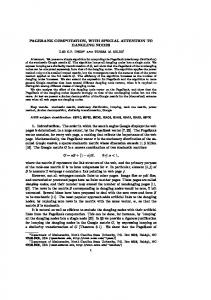
the syntactic theory of linguistics where prose is built up from well-defined vocabularies of discrete elements that are arranged according to syntactical rules, and can be unambiguously parsed into phrases, (Chomsky, 2002). Stiny argues that this approach has little in common with how designers actually perceive shapes and argues that a shape is not a fixed set of elements but that a dynamic reinterpretation of shapes is vital, (Stiny, 2006). Under a linguistic approach to design this is not possible and emergent shapes cannot be recognised or manipulated in a design. For example, the shape in Figure 2.1 is a familiar and widely used example of the ambiguity of emergent shapes and can be interpreted in a number of different ways, e.g. it can be considered to be composed of two squares or alternatively two L’s. However, if a linguistic model is applied and the shape is initially
Figure 2.1: Two squares or two L’s?
composed of two squares then the subshapes that emerge as a result of the interaction between the two squares are not recognised and, in fact, do not exist. Stiny argues that a shape is composed of whatever elements the designer cares to see, be they squares, L’s or indeed any other subshapes embedded in the shape. This approach to shape representation is more suited to the interactive sketching process and suggests a more natural model for computational design.
2.4
Generative Design
In the previous section it was stated that design problems can be computationally regarded as search problems. However, Earl notes that although standard CAD systems allow for simulation and visualisation of designs, and provide pictures of instances of objects in a design space that can be individually analysed, they do not provide a means to explore freely the design space, (Earl, 1999). Alternatively, generative methods of design
20 are explicitly concerned with defining and exploring the space in which search takes place. McCormack et al. note that although a generative approach to design requires that designers reconsider their approach to designing, it also provides certain advantages over more traditional approaches, (McCormack et al., 2004a). In a generative approach, designers are no longer manipulating a static representation of a design directly, but rather are manipulating, via rules or systems, the dynamic process that generates the representation. In return, unexpected design solutions can be generated that fall outside of a designer’s expectations. This was illustrated by March who generated a range of unexpected designs via the application of a simple shape rule that manipulates equilateral triangles, (March, 1996). Similarly, Woodbury and Burrow note that designers often utilise successful design decisions from the past in future projects, and that generative methods provide an explicit means of encoding these decisions in terms of design spaces that record alternatives that were rejected, (Woodbury and Burrow, 2004). For example, the SEED (Software Environment to Support Early Phases in Building Design) project is concerned with developing a software environment that supports the rapid generation of design representations, (Flemming and Woodbury, 1995). Unlike traditional CAD programs SEED provides conceptual design alternatives and variations for evaluation, and provides systematic support for the storing and retrieval of past solutions and their adaptation to similar problems. In general, generative systems of design are based on the combinatorial models of design discussed in the previous section and while a certain amount of success has been achieved in generating restricted classes of design, such as very large scale integrated (VLSI) circuit designs, the extension of this success to more general classes of design has proven to be a difficult problem. VLSI design lends itself to generative methods because, as Whitney illustrates, the design of a VLSI circuit can be considered a modular process, (Whitney, 1996). A VLSI design is composed of individual device elements that are connected according to specified design rules that impose limits on their geometry. The device elements are designed at a component level, where they are verified to ensure they behave as required, and are stored in a device library. Each device element performs a single logical function and its behaviour essentially remains unchanged when it is incorporated into a system. There is no unwanted interaction between elements such
2.4 Generative Design
21
as back loading because information or control is passed in one direction only, and the design rules eliminate unwanted side effects such as crosstalk. As a result the design of a specific product at a system level can be built up bit-by-bit in building-block fashion, where elements are added as functions are required and the functional specification of the final product can be verified via consideration of the function of the components, (Barrow, 1984). This modular approach to design is well suited to combinatorial models which have been successfully applied to automate the generation of VLSI designs, (Gerez, 1999). The effectiveness of synthesis methods in VLSI design has inspired the application of similar approaches in mechanical design. According to Whitney these approaches will not be successful since mechanical design is inherently different from VLSI design. Components of a mechanical design are usually multi-functional and designers often rely on this multi-functional nature in order to obtain efficient designs, for example rotating elements transmit shear loads whilst also storing rotational energy. However, multi-functional behaviour can induce side effects, such as fatigue, that can have unwanted consequences with regards to other components of the system. These side effects can result in components behaving differently in a system to how they behave in isolation. As a result, components cannot be designed independently of each other or indeed independently of the system, and reuse of components in different systems is complicated. Thus a modular approach to mechanical design is inappropriate, and combinatorial models of design are insufficient for mechanical design compilation. Indeed, following Whitney’s argument, it seems that combinatorial models are insufficient to model any design processes that cannot be considered modular. Although Whitney’s conclusions concerning the future of generative systems in design are not encouraging this view is not generally shared by the research community at large. For example, Antonsson responded to Whitney’s negative remarks by claiming that “significant potential exists for the development of approaches to compilation of mechanical design systems”, (Antonsson, 1997a). He argues that certain sub-domains of mechanical design can be considered to be modular processes and as a result are suitable for combinatorial modelling. As an example he cites Ward’s mechanical compiler of hydraulic systems and suggests that similar methods can be applied to areas of mechanical design
22 that are dominated by assembly of components, (Ward, 1989). Antonsson also suggests that while early developments in generative design have largely generated modular designs future work will produce more integral designs, (Antonsson, 1997b). However, the combinatorial models on which generative systems are generally based pose intrinsic difficulties for the generation of non-modular designs. Instead, the shape grammar formalism on which this thesis is based provides an alternative, non-modular, approach to design generation.
2.5
Design Generation with Shape Grammars
Shape Representation Shape grammars are a formal production system, equivalent to a Turing machine, whereby languages of shapes or designs are generated according to shape replacement rules, (Stiny, 1980). In this context, a shape is an arrangement of a finite number of spatial elements, each with a definite boundary and limited but non-zero extent, such as points, lines or planes. These spatial elements are said to be embedded in the shape. Shape grammars differ from most other computational systems of design in that the components of a shape are not fixed but change dynamically throughout a computation. Any shape, with the exception of shapes composed of isolated points, can be decomposed into spatial elements in an unlimited number of ways and each decomposition provides a representation of the shape. For example, in Figure 2.2 three representations of the shape from Figure 2.1 are illustrated, although uncountably more exist.
Figure 2.2: Representations of the shape in Figure 2.1
This liberal nature in which shapes can be represented leads to difficulties when it is necessary to describe a shape uniquely, for example in shape computations. Difficulties
2.5 Design Generation with Shape Grammars
23
arise because the task of determining whether or not two representations refer to the same shape can be computationally expensive, if not impossible. As a result it is desirable to avoid this ambiguity by providing a consistent representation of shapes that describes all visually similar shapes in a unique, canonical way. This is achieved by representing a shape according to its maximal spatial elements. Two spatial elements can be merged to form a single spatial element if they are co-equal and they overlap or share a boundary. For example, two co-linear lines that overlap or share an end point can be merged to form a single line, or two co-planar planes that overlap or share a boundary can be merged to form a single plane. Otherwise, the spatial elements are said to be maximal with respect to each other. The representation of a shape in which all spatial elements are respectively maximal, called the maximal representation, provides a unique, canonical representation of the shape. For example, consider the shape representations in Figure 2.2. The second and third representations are clearly not maximal since they contain co-linear lines that share end points. Conversely, all the lines that compose the first representation are maximal with respect to each other and as a result, this is the maximal representation, and it provides a unique canonical representation of the shape. Arrangements of spatial elements embedded in a shape are said to be subshapes of the shape and, since there is no restriction on how a shape can be decomposed into spatial elements there is similarly no restriction on how a shape can be decomposed into subshapes. As a result, in a shape grammar formalism, shapes are not represented by components enforced by the system. Instead a shape is defined within an algebra, according to the subshapes and spatial elements embedded in the shape, Stiny (1991). A shape is said to be a subshape of a second shape if all of the maximal elements of the first can be embedded in the maximal elements of the second. For example, a square is a subshape of the shape from Figure 2.1 since there are three examples of squares embedded in the shape, as illustrated in Figure 2.3. A subshape that is common to all shapes is the empty shape which is defined as the shape in which there are no spatial elements. When describing shapes in terms of spatial elements shapes composed of isolated points stand out as an exception. Whereas all other types of spatial element can always be decomposed into multiple elements of the same type, points are by definition atomic and
24
Figure 2.3: Some subshapes of the shape in Figure 2.1
cannot be further decomposed. That is, a line can always be decomposed into multiple lines, or a plane can always be decomposed into multiple planes, but a point cannot be decomposed. As a result, whereas shapes composed of lines or planes can be decomposed into subshapes in an unlimited number of ways shapes composed of a finite number of isolated points only have a finite number of decompositions. For example, in Figure 2.4 the subshapes of a shape composed of three isolated points are enumerated, and in total there are eight subshapes, including the original shape and the empty shape. Shape grammars
Figure 2.4: All subshapes of a shape composed of three points
involving shapes composed of isolated points are analogous to the combinatorial models of design previously discussed, where designs are composed of individual modules. On the other hand, shapes grammars involving shapes composed of any other type of spatial element (possibly in combination with isolated points) avoid this combinatorial representation, and allow a more natural approach to design, where shapes can be decomposed according to the perception of the designer.
Shape Grammars A shape grammar consists of an initial shape and a set of rules of the form α → β, where α and β are both shapes, as illustrated in Figure 2.5. A rule is applicable to a
2.5 Design Generation with Shape Grammars
25
Figure 2.5: An example shape rule
shape γ if some similarity transformation of the shape α on the left hand side of the rule is a subshape of γ, denoted α ≤ γ, where ≤ is the subshape relation. Application of the rule removes the instance of the subshape α and replaces it with a similarly transformed instance of the shape β on the right hand side of the rule. For example, the shape rule in Figure 2.5 removes a square and replaces it with a rotated square. This rule can be applied to the shape in Figure 2.1 by first recognising any of the three squares embedded in the shape. The embedded square is then removed and replaced with a rotated square. Repeated application of the rule produces the shapes in Figure 2.6.
Figure 2.6: Results of rule application
Shape grammars are based on Post production systems, where replacement rules are used to generate a language of strings, (Post, 1943). These production systems are also the basis for phase structure grammars from which modern linguistic theory has been developed, (Chomsky, 2002), and as a result shape grammars are often criticised for applying a linguistic analogy to design, (Flemming, 1994). However, this is not true and it is important to note the difference between shape grammars and linguistics. Linguistic theory is concerned with languages of objects (words) that are composed of a finite number of discrete elements (symbols). Shape grammars on the other hand are concerned with languages of objects (shapes) that are composed of a finite number of discrete elements
26 (maximal spatial elements) that, with the exception of points, can always be further decomposed into constituent elements. This distinction means that whereas in linguistics it is possible to decompose an object into its primitive atoms, in shape grammars there are no fixed primitives and there is no limit on how an object can be decomposed. As a result, any shape can be decomposed into subshapes in an unlimited number of ways, and any subshape can be operated on through application of shape rules. This gives rise to one of the main strengths of shape grammars, namely their ability to generate, recognise and operate on emergent shapes. Emergent shapes are not explicitly defined in an initial shape or in the shape rules of a grammar, instead they materialise during a computation as a result of rule application. They are often unexpected and recognition of such shapes can suggest new directions in which to explore a design space. Emergent behaviour is not unique to shape grammars and is exhibited by many other computational systems. For example, Conway’s Game of Life is a cellular automaton whereby simple rules applied to single cells arranged in a grid result in surprising emergent patterns, (Gardner, 1983). However, Knight points out that emergence in shape grammars is inherently different from the emergence seen in most other computational systems, (Knight, 2003). Emergence in systems such as the Game of Life occurs at a global level as a result of the behaviour of atomic elements at a local level. While emergence in these systems can be generated and observed the emergent phenomena are generally the output of the system and are not usually recognised and utilised in further computations. Conversely, emergence in shape grammars occurs at a local level where shapes are formed that are not explicitly represented in the initial shape or in the rules that are applied during computation. For example, the second and fourth shapes in Figure 2.6 both contain a triangle that is not identified in the initial shape in Figure 2.1, or in the rule that is applied to it, Figure 2.5. Such emergent shapes are a foundational feature of computation with shape grammars and enhance shape exploration. For example the shape rule in Figure 2.7 will recognise the triangles in the shapes in Figure 2.6 and can be applied to further explore the shapes. This reflects the flexible modes that are utilised by designers when manipulating pictorial representations such as sketches. Some extensions of the basic shape grammar formalism have also been defined including
2.5 Design Generation with Shape Grammars
27
Figure 2.7: A second shape rule
labelled shape grammars and parametric shape grammars, (Stiny, 1980). With labelled shape grammars aspects of a shape are distinguished by labels which are utilised to direct the generation of designs and reduce the extent of a design space. On the other hand, parametric shape grammars expand the design space since they are composed of rules that can be applied to a family of shapes which are defined by a parameterised shape. For example, a square, when considered as a parametric shape, can define the family of quadrilaterals, and under a parametric shape grammar formalism the shape rule in Figure 2.5 can be applied to rotate any of the three quadrilaterals embedded in the shape in Figure 2.8.
Figure 2.8: A shape composed of quadrilaterals
Applications of Shape Grammars The initial application of shape grammars was as a system for formalising aesthetic qualities and they were used to generate geometric paintings and sculptures, (Stiny and Gips,
1972). Since then however they have generally been adopted as a system for
generative designs in a range of design fields. As previously discussed, design can be viewed as a problem solving activity involving the formulation of a space of possible solutions and a search through the space. Shape grammars provide a formal description of the design space in terms of shapes, and provide a means of exploring design possibilities. The majority of published work on shape grammars has been concerned with formal-
28 ising established styles of architectural design in order to generate original designs in the same style. The earliest of these works is Stiny and Mitchell’s shape grammar inspired by Palladio’s rules of architecture, which generates villa ground plans in the Palladian style, (Stiny and Mitchell, 1978). March and Stiny point out that this grammar characterises stylistic similarities by clarifying the underlying structure and appearance of known instances of the style, by supplying the conventions and criteria necessary to recognise whether any other design is an instance of the style, and by providing the compositional machinery needed to generate new instances of the style, (March and Stiny, 1985). Indeed, the Palladian grammar has been utilised to generate original designs, which have been accepted by expert architects as true instances of the Palladian style. Similarly, Koning and Eisenberg developed a shape grammar that incorporates design principles specified by Frank Lloyd Wright in order to generate prairie-style houses (Koning and Eizenberg, 1981). The architecture of Wright’s prairie-style houses have long been considered mysterious and difficult to decipher and this grammar is able to provide a formal interpretation of the style in terms of shape. The Wright grammar also meets the three conditions characterising the definition of style outlined by Stiny and March. Other examples include grammars that capture the landscape architecture of Mughul gardens, (Stiny and Mitchell, 1980), and the architectural styles of Giuseppe Terragni, (Flemming, 1981), the bungalows of Buffalo, (Downing and Flemming, 1981), Japanese tea rooms, (Knight, 1981), Glenn Murcutt, (Hanson and Radford, 1986), Queen Anne houses, (Flemming, 1987b), Christopher Wren, (Buelinckx, 1993), Taiwanese traditional houses (Chiou and Krishnamurti, 1995), Chinese hall sections, (Li, 2004), Alvaro Siza, (Duarte, 2005), and Chinese bracket systems, (Wu, 2005). As illustrated, shape grammars have proved to be a successful system for generating the rectilinear forms so often seen in architecture but applications outside of architecture are relatively few. Dumont and Wallace suggest that this is because the shape grammar formalism does not readily support freeform design, (Dumont and Wallace, 2003). However, some notable examples of shape grammar applications in design fields such as engineering design have been developed, a review of which is given by Cagan (2001). These applications include Brown’s parametric lathe grammar which uses the method of shape
2.5 Design Generation with Shape Grammars
29
annealing in conjunction with shape rules that specify the language of shapes manufacturable on a simplified axisymmetric lathe in order to produce cost efficient manufacturing process plans, (Brown and Cagan, 1997). Similarly, Shea’s space truss grammar utilises shape annealing to produce manufacturable structural designs that meet specified stress and boundary requirements, (Shea, 1997). Also of note is Agarwal and Cagan’s parametric coffee maker grammar, which is one of the few applications in the field of consumer product design, (Agarwal and Cagan, 1998). The coffee maker grammar meets the three conditions characterising the definition of style outlined by Stiny and March and applies them in order to define brand identity. These three examples illustrate the potential for the application of shape grammars in engineering design. However, Cagan notes that the majority of engineering design grammars are not driven by the emergent properties of shape, but instead are driven by labels. They are examples of set grammars which are defined by Stiny as a combinatorial approach to the shape grammar formalism, (Stiny, 1982). This approach allows the functional subsystems of a design to be developed individually within a design, for example in the coffee maker grammar the coffee pot, filter and water storage are each generated as individual subsystems. In architecture, functional subsystems such as rooms can be developed in a more holistic manner in terms of overlapping and emergent shapes, and Cagan suggests that engineering design will also benefit from such an approach. Recently, some developments have been made in terms of engineering design grammars that take advantage of emergent curvilinear shapes. Chau et al. developed parametric shape grammars that define the brand identity of consumer packaging, namely coca-cola bottles and shampoo bottles, (Chau et al., 2004), and similarly McCormack et al. developed a parametric shape grammar that defines the brand identity of Buick cars, (McCormack et al., 2004b). Both of these works utilise shape grammars in order to generate curvilinear designs. However, both works treat shape grammars with curves as a direct extension of shape grammars with straight lines. No consideration is given of the formal structures that are necessary to provide a framework for computation with curved shapes. Also, the packaging grammars, while allowing for recognition of emergent shapes, are restricted to working with regular circular arcs and do not appear to support more
30 freeform curves. The Buick grammar on the other hand does support shape generation with freeform curves, but does not utilise the emergent properties of shapes. The grammar supports shape matching by considering an underlying structure composed of straight lines, and issues concerning curve embedding have not been considered, (McCormack and Cagan, 2003). Curves are of an intrinsically different nature to straight lines and consequently shape grammars applied to curved shapes need not necessarily be a simple extension of shape grammars applied to straight lines. A general discussion concerning the maximal representation of curved shapes and the issues concerning curve embedding was presented by Jowers et al. (2004). However, in order for shape grammars to take advantage of the embedding properties of freeform shapes further work is needed. In the remainder of this thesis issues regarding the implementation of shape grammars on curved shapes will be addressed. In Chapter 3, the formal structures of shapes composed of freeform shape are developed by considering algebras of shapes composed of freeform spatial elements. In Chapter 4, implementation issues for shape grammars are considered, and algorithms are developed that enable the implementation of shape grammars on shapes composed of parametric curve segments. In Chapter 5 and Chapter 6, these algorithms are applied in order to implement shape grammars on shapes composed of quadratic and cubic B´ezier curves, respectively. Finally, in Chapter 7 a discussion is presented concerning the application of curved shape grammars in design.
2.6
Summary
The discipline of computational design is concerned with formalising the design process in order to make it more visible and comprehensible. This goal has been achieved to a certain extent by representing the process in terms of combinatorial models. However, it is commonly accepted that design is not combinatorial in nature and as a result these models will never fully capture the intricacies of the design process. Shape grammars provide an alternative non-combinatorial approach to modelling design in terms of shapes and shape rules. Initial definitions of shape grammars were in terms of shapes composed of straight
2.6 Summary
31
lines and as a result they have proved to be successful in generating designs composed of rectilinear forms such as those commonly seen in architecture. Applications in design fields where designs are more freeform, such as industrial design, are less common. The few examples that exist in engineering design illustrate the promise of such an approach to modelling the design process however these works adopt two different approaches that do not take full advantage of the shape grammar formalism. The first approach is a combinatorial approach where designs are generated via set grammars, and the emergent properties of shapes are not considered. The second approach considers shape grammars with curved shapes as a direct extension of shape grammars with straight lines. Issues concerning the formal structures underlying shape grammars with curved shapes and the difficulties inherent in the embedding properties of curves have not been satisfactorily discussed. This thesis addresses these issues. First, the formal structures underlying the shape grammar formalism will be investigated and extended in order to allow for application to shapes composed of freeform spatial elements. Then, these developments will be utilised in order to propose practical solutions to the problems concerning the implementation of shape grammars with shapes composed of curve segments.
Chapter 3
Algebras of Freeform Shapes 3.1
Introduction
As discussed in the previous chapter, pictorial representations, such as sketches or CAD models, play an important role in many design processes. These processes can be modelled by shape computations that formalise the manipulation of pictorial representations in the pursuit of a solution to a specific design problem. For example, design of a product to meet a functional need or create a particular response is achieved through manipulation of elements such as components and form lines, (Prats and Earl, 2006). These elements are moved, added, deleted, stretched, transformed etc. until the design serves to achieve its goal. The methods of shape manipulation that are commonly utilised were discussed by Mitchell and can be generalised in terms of spatial transformations and Boolean operations, (Mitchell, 1990, chapter 7). Spatial transformations are unary operations that operate on single shapes, whereas Boolean operations are binary and operate on two shapes to produce a third. Shape manipulations serve both to generate and to explore design worlds, comprising shapes of a particular type or class, and these processes can be formalised as a sequence of rules in a shape grammar, (Stiny, 1980). When manipulating shapes of a particular class within a shape computation it is formally required that the resulting shapes are also of the same class so that further manipulation can take place. In other words, it is required that shapes and the operations applied to them form a closed algebra. For example, when manipulating polygons in a CAD system it is desirable that the resulting shapes are also polygons. However, Tilove
3.2 Algebras of Shape
33
and Requicha point out that, in CAD systems, geometric entities of particular interest are represented by point sets and are usually not closed under conventional operators, (Tilove and Requicha, 1980). Instead, they suggest the use of regularised operations to ensure closure. Similarly Stiny demonstrated that if shapes are represented by their maximal spatial elements then they form algebras, called shape algebras, that are closed under Euclidean transformations and Boolean operations, (Stiny, 1991). Shape algebras formalise the shapes, shape operations and spatial transformations utilised in shape computations. The advantages of a shape algebra representation of shapes over other representations, such as point set representations, have been discussed by Chase (1996). The most prominent of these advantages is that such a representation enables the emergence of features that are not apparent in the initial formulation of a shape. As discussed in the previous chapter, this ability to recognise and manipulate emergent shapes facilitates the exploration of a design space. Initial definitions of shape algebras are for shapes composed of points, lines, planes or solids that are arranged in Euclidean spaces of different dimensions. In this chapter these initial definitions will be extended to include shapes composed of freeform spatial elements arranged in freeform spaces such as curves, surfaces and curves embedded in surfaces. Such an extension will increase the scope of applicability of shape grammars to include more freeform shapes, as discussed by McCormack and Cagan (2003), and Jowers et al. (2004). In these extended algebras, shapes will be distinguished from each other not only by the dimension of the space in which they are arranged and the dimension of the spatial elements of which they are composed, but also by the type of the spatial elements and the type of space in which they are arranged.
3.2
Algebras of Shape
Within the framework of shape computation, a shape is defined as an arrangement of a finite number of spatial elements, each with a definite boundary and limited but non-zero extent. These spatial elements, with the exception of isolated points, can be decomposed into finite sets of parts, which are themselves spatial elements of the same type. For
34 example, a straight line can be decomposed into finite sets of straight lines. Different decompositions of spatial elements lead to different decompositions of a shape into subshapes which can in turn be further decomposed into sub-subshapes. As a result, a shape defines a distributive lattice which represents the partial order of the subshape relation. For example, in Figure 3.1 the distributive lattice of a shape composed of three isolated points is illustrated. This lattice can naturally be extended to include all shapes composed
Figure 3.1: Distributive lattice of a shape composed of three points
of points arranged in a plane by noting that the three points are subshapes of other shapes composed of points. This extension results in an infinite lattice of subshapes where the shape operations union, product and difference are in turn formally defined by the subshape relation, (Stiny, 2006). The lattice is equivalent to an algebra of shapes composed of points arranged in a plane and algebras of shapes composed of other spatial elements are similarly defined. These algebras are closed under finite applications of the Boolean operations of union (+), product ( · ) and difference (−), and the shapes in the algebra are partially ordered by the part relation (≤). It has been demonstrated by Stiny that shape algebras for shapes composed of points, straight lines, planes or solids have most of the properties of a Boolean algebra but in general fail to be one, lacking a unit and complements, (Stiny, 1993). However, there is one exception to this rule. A shape that is composed of a single point in a zerodimensional space, i.e. a point space, has both a unit and a complement. In this case, the
3.2 Algebras of Shape
35
algebra is indeed a Boolean algebra. All other shape algebras are equivalent to a Boolean ring with the empty shape for the zero and no unit. This theory of shape algebras is an application of the mathematical theory of mereology which is a formal study of the logical properties of the relation of whole and part, (Simons, 1987). In particular, the algebra of parts developed by Bostock, for objects which are non-continuous, shares many of the properties of the shape algebras proposed by Stiny, (Bostock, 1979). However, there are some notable differences between the algebras, including the absence of null objects in Bostock’s algebras. The simplest shape algebras defined by Stiny contain shapes composed of a single type of spatial element that are arranged in a specific Euclidean space. In Figure 3.2, these algebras are enumerated up to solids defined in three-dimensional space. Here, shapes U00
U01
U02
U03
U11
U12
U13
U22
U23 U33
Figure 3.2: Algebras of shapes
in an algebra Uij are composed of spatial elements of dimension i that are arranged in a Euclidean space of dimension j, and the algebras serve to distinguish between these categories of shape or, in the terminology of Earl, between these different design worlds, (Earl, 1986). For example, a straight line sketch on a sheet of paper is a planar shape in an algebra U12 , whereas a wire frame model that is composed of straight lines in a three-dimensional space is in an algebra U13 . More complicated algebras containing shapes composed of multiple types of spatial elements arranged in multiple spatial dimensions are defined by the Cartesian product of two or more of the simple algebras given in Figure 3.2. The Cartesian product of two algebras Uij and Unm , denoted Uij × Unm , is defined to be the algebra of all shapes (a, b) where a is a shape in the algebra Uij and b is a shape in the algebra Unm . For example, a wire frame edge model with planar polygon surface facets is in an algebra U13 × U23 . In a composite algebra, spatial elements from different simple algebras are
36 kept as separate components of the shape. For example, if linear elements a and c are in an algebra U13 and planar elements b and d are in an algebra U23 then the composite algebra U13 × U23 contains the shapes (a, b) and (c, d), where elements in U13 are separate from the elements in U23 . Operations applied to the shapes will also keep the elements from different simple algebras separate. For example, the union of the two shapes (a, b) and (c, d) is defined as (a, b) + (c, d) = (a + c, b + d), the product of the two shapes is defined as (a, b) · (c, d) = (a · c, b · d), and the difference between the two shapes is defined as (a, b) − (c, d) = (a − c, b − d).
3.3
An Algebra of Planar Freeform Shapes
The initial definitions of shape algebras are for shapes composed of points, lines, planes and solids, (Stiny, 1991). However, in design fields such as industrial design, it is common for pictorial representations to be composed of shapes of a more freeform nature and as a result it is desirable to extend these algebras to include shapes composed of freeform spatial elements. Here, freeform shapes are defined to be characterised by flowing forms resulting from spatial elements with varying intrinsic properties, and are in contrast to regular shapes composed of spatial elements with constant intrinsic properties such as polygons or circles. An understanding of the properties of these extended algebras can be gained by comparing shapes composed of curved spatial elements with shapes composed of rectilinear spatial elements. For example, a sketch composed of curve segments on a sheet of paper, such as the car design composed of circular arcs in Figure 3.3, is comparable to a planar shape composed of straight lines. Both are shapes composed of one-dimensional
Figure 3.3: A planar shape composed of circular arcs
spatial elements that are arranged in a two-dimensional Cartesian space, and as such both belong in an algebra U12 . However, straight lines and circular arcs have different
3.3 An Algebra of Planar Freeform Shapes
37
embedding properties and are of different generalised types. Accordingly, shapes composed of straight lines and shapes composed of circular arcs should be in different algebras. A discussion concerning the types of spatial elements follows shortly. Conceptually, the algebra of shapes composed of straight lines in a plane, say U12 (lines) is similar to the algebra of shapes composed of circular arcs in a plane, say U12 (arcs). In both algebras, shapes are composed of a finite number of spatial elements which have a definite boundary and finite non-zero length. However, note that while straight lines always have a boundary defined by a shape composed of two points this is not always true for circular arcs. If the length of an arc is greater than 2πr, where r is the radius of the arc, then the arc contains its endpoints and forms a closed shape, a circle, with its boundary as the empty shape. Otherwise, if the length of an arc is less than 2πr, then its boundary is defined comparably to that of a straight line, by a shape composed of two points. The algebras U12 (lines) and U12 (arcs) are closed under the Euclidean transformations translation, rotation, reflection and isotropic scale, and the Boolean operations of union, product and difference and the shapes in the algebras are ordered by the part relation. They have no unit and no complements and in each case the algebras are a distributive lattice that are equivalent to Boolean rings. More general algebras in which shapes can be composed of both circular arcs and straight lines are defined by the Cartesian product of the algebras U12 (lines) and U12 (arcs). For example, the car design in Figure 3.4 is composed of straight lines and circular arcs arranged in a plane and is in a composite algebra U12 (lines) × U12 (arcs). This composite algebra can also be written as U12 (lines & arcs).
Figure 3.4: A planar shape composed of lines and arcs
The definition of shape algebras can also be extended to include shapes that are composed of more freeform curves in a plane. For each type of planar curve, denoted by
38 the variable elements, there exists an algebra U12 (elements) that contains planar shapes composed of curve segments of that type. These algebras possess the same properties exhibited by the algebras U12 (lines) and U12 (arcs). That is, the algebras U12 (elements) are equivalent to Boolean rings with shapes partially ordered by the subshape relation. These general algebras can also be combined to form composite algebras in which shapes are composed of more than one type of freeform curve. For example, a general algebra that contains shapes composed of any type of curve arranged in a plane is given by the Cartesian product U12 (elements1 ) × U12 (elements2 ) × . . . × U12 (elementsn ) and can be written as U12 (all elements), or simply U12 .
3.4
A Discussion on type
In this chapter, algebras of shapes composed of freeform spatial elements are distinguished by comparing a property of the spatial elements that is here referred to as type. Krishnamurti states that any finite spatial element can be represented according to a descriptor and a boundary, (Krishnamurti, 1980). The descriptor defines the carrier of a spatial element, the geometric object of infinite extent in which the element is embedded, and the boundary defines the location of a spatial element on its carrier. The property of type defines an equivalence class of descriptors which is closed under a specific set of transformations. Therefore, two spatial elements are of the same type if they lie on carriers that are equivalent under this specified set of transformations, which is in turn dependent on the algebra in which the spatial elements are arranged. For example, if an algebra is specified to be closed under Euclidean transformations, as is the standard in shape grammars, then the two curves in Figure 3.5 will be considered to be of different types because their carriers are equivalent under a shear transformation, which is not a Euclidean transformation. If however, the algebra is specified to be closed under Euclidean transformations augmented by shear transformations then the two curves will be of the same type. In this work it is assumed that an algebra contains all shapes that can be composed of a specific type of spatial element, arranged in a specific space. This assumption is necessary in order to place a limit on what can be considered as an algebra, and requires a
3.4 A Discussion on type
39
Figure 3.5: Two curves, equivalent under a shear transformation
minimal requirement on the transformations under which an algebra is said to be closed. For example, the transformations under which the algebra U01 (line) is closed must include translation since translation is enough to ensure that all shapes composed of points in a line are in the algebra. Similarly, the transformations under which the algebra U12 (arcs) is closed must include translation, rotation and isotropic scaling since a combination of these transformations is enough to ensure that all planar shapes composed of circular arcs are in the algebra. The definition of spatial element type used here is analogous to Mitchell’s definition of shape type, where shapes are of the same type by virtue of having something in common, such as relationships between spatial elements, (Mitchell, 1990, chapter 6). For example, all equilateral triangles can be considered to be of the same type because they are polygons composed of three lines of equal length. Shape types are also dependent on associated sets of transformations. For example, the shape type “equilateral triangle” is closed under Euclidean transformation but not under a shear transformation. As Mitchell states, the concept of type, equivalence and closure are inseparable. Formally, a weak definition of spatial element type can be stated as follows. Two spatial elements a and b are of the same type if there exists a third spatial element c and allowable transformations t1 and t2 such that t1 (a) ≤ c and t2 (b) ≤ c. Clearly, in such a case the spatial elements a, c and b, c lie on carriers that are equivalent under the transformations t1 and t2 , respectively. For example, if an algebra is defined such that it is closed under a transformation that maps straight line segments onto circular arcs then straight lines and circular arcs are of the same type. Consequently, a straight line and a circle are also both of the same type because there exists a spatial element, namely a circle, in which both the straight line and the circle can be embedded under some allowable
40 transformation. Note that, when considering topologically distinct spatial elements such as circles, which are closed, and straight lines, which have infinite extent, this definition of type is not diffeomorphic since although a straight line can be embedded in a circle, it is unclear how a circle can be embedded in a straight line, without loss of information. Clearly, this definition of type requires further development but it is sufficient in order to formalise the shape computations explored in the remainder of this thesis, where shapes are composed of spatial elements that are topologically equivalent. In the previous section concerning algebras of shapes composed of circular arcs in a plane it was assumed that the allowable transformations were Euclidean and as a result, straight lines and circular arcs were introduced as examples of different types. Types of specific spatial elements can be compared to each other by considering their intrinsic properties, since these properties capture the embedding properties of spatial elements without reference to their spatial properties, (Attneave, 1954). For example, the intrinsic properties of planar curves are defined by their curvature, and the intrinsic properties of space curves are defined by their curvature and torsion. Comparison of these properties within the allowable transformations will determine whether or not two spatial elements are of the same type. For example, under Euclidean transformations, straight lines that have a zero curvature are of a different type from circular arcs that have a constant non-zero curvature, and both are of a different type from more freeform curves that have varying curvature. Types form either disjoint sets or embedded sets of spatial elements. That is, two types T1 and T2 do not have some but not all spatial elements in common. Either the types are defined such that T1 and T2 have no spatial elements in common, or they are defined such that the spatial elements in T1 form a subset of the spatial elements in T2 or vice-versa.
3.5
Algebras of Shapes in One-Dimensional Space
Further understanding of the properties of algebras of freeform shapes can be gained by considering shapes arranged in spaces of different dimensions, such as shapes arranged in
3.5 Algebras of Shapes in One-Dimensional Space
41
one-dimensional space. For example, shapes in Stiny’s U11 algebra are composed of straight line segments that are arranged in a Euclidean one-dimensional space, i.e. a straight line. A natural extension of this algebra would incorporate shapes that are composed of freeform curve segments arranged in a one-dimensional space. However, algebras U11 that include curve segments are not so easily defined as the algebras U12 that include curve segments. This is due to the different embedding properties of curves and straight lines. Curves are intrinsically and, in some cases, topologically different from straight lines and as such cannot be arranged in a linear one-dimensional space. But since curves, like lines, are onedimensional spatial elements it is expected that they, like lines, can form shapes in a onedimensional space. Therefore, in order to define algebras U11 that include curved shapes it is necessary to consider definitions of space other than the Euclidean definition. For example, while circular arcs cannot be arranged in a standard Euclidean one-dimensional space, they can be arranged in a circular one-dimensional space, as illustrated in Figure 3.6. Accordingly, shapes composed of different types of curves are in different algebras
Figure 3.6: Arc segments in a circular one-dimensional space
U11 (space), where the variable space represents the type of one-dimensional space in which the shapes are arranged. Here, the type of space is analogous to the type of spatial element previously discussed and spaces of the same type are equivalent under transformations that are allowable in a specific algebra. Consequently, the types of one-dimensional spatial elements that can be arranged in a one-dimensional space are dependent on the type of the space. Shapes composed of points can also be arranged in different types of onedimensional space. These shapes are in the algebras U01 (space). The shape algebras U11 (space) have different properties depending on the topological and intrinsic differences of the types of spaces in which shapes are arranged. For example, when space refers to a closed space, such as a circular space, it is topologically different
42 to a space of infinite extent such as a linear space. A closed space is of finite extent and as a result a shape defined in this space has a complement, as illustrated in Figure 3.7(b) for a circular space. Also, since the space is of finite extent it can itself, by definition, be
(a) A shape C in circular space
(b) C 0 , the Complement of C
(d) C − C 0 = C
(c) C + C 0 = I
(e) C · C 0 = 0
Figure 3.7: Boolean algebra of a shape C in circular space
considered to be a shape, and serves as the unit of the algebra, as illustrated in Figure 3.7(c). As a result, algebras U11 (space) where space is a closed shape have all the properties of a Boolean algebras, as illustrated in Figures 3.7(a) - 3.7(e). On the other hand, as discussed previously, the algebra U11 (space) where space is a straight line is lacking a unit and complements and is equivalent to a Boolean ring. This distinction is similar to the distinction previously made between the algebra U00 , for a shape composed of a single point in a zero-dimensional Euclidean space, and algebras for shapes in higher dimensional Euclidean spaces. Intrinsic differences in one-dimensional spaces result in the shape algebras U11 (space) being closed under different transformations. For example, the algebras of shapes arranged in a linear space U11 (line), are closed under Euclidean translation but the algebras U11 (space) where space is the curve in Figure 3.8 are not. Euclidean translations are a rigid body transformation and preserve the shape of a spatial element, whereas a “translation” in the algebras U11 (space) can distort the shape of a spatial element according to the intrinsic properties of space, as illustrated in Figure 3.8 by the transformation between
3.5 Algebras of Shapes in One-Dimensional Space
43
Figure 3.8: “Translation” in a non-Euclidean one-dimensional space
the curve segments c1 and c2 . It is interesting to note the similarity between the one-dimensional space in which the shapes in an algebra U11 (space) are arranged and the carrier of the curve segments that compose the shapes. The carrier of a curve segment is the infinite curve (or possibly finite if the carrier forms a closed shape) on which the segment lies. Similarly, a one-dimensional space is an infinite curve (or possibly finite if the space forms a closed shape) in which curve segments are arranged. Clearly, from their definitions, there is an equivalence between the carrier of a curve and the one-dimensional space in which it can be arranged. Composite algebras in which shapes are composed of a combination of one-dimensional spatial elements and points, arranged in a specific type of one-dimensional space can be defined by the Cartesian product of the algebras U11 (space) and U01 (space). For example, Edwin Abbott’s vision of Lineland, illustrated in Figure 3.9, is a shape in the composite algebra U01 (line) × U11 (line), (Abbott, 1884). However, since a one-dimensional spatial
Figure 3.9: Abbott’s Lineland
element can only be embedded in a one-dimensional space of the same type, it is not possible to define a composite algebra in which one-dimensional elements of more than one type can be arranged in the same one-dimensional space. The Cartesian product of algebras in which one-dimensional shapes are arranged in spaces of different types will be discussed later.
44
3.6
Algebras of Shapes in Two-Dimensional Space
It has been shown that algebras of shapes arranged in one-dimensional space need not be limited to shapes arranged in a Euclidean space, but can also be defined for shapes arranged in different types of one-dimensional space. Similarly, shapes in two-dimensional space need not be arranged in a two-dimensional Euclidean space. For example, Grossman et al. discuss a computational system whereby principle 3D curves are arranged on the surface of a full scale car model, (Grossman et al., 2002). Here, shapes are arranged in a non-Euclidean two-dimensional space that is defined by the surface of the car model. Similarly shapes can be arranged in any two-dimensional space, such as the surface of a cylinder, sphere or cone. This is illustrated in Figure 3.10, where a graphical design is arranged on the surface of a mug, i.e. the shapes are arranged in a non-Euclidean, cylindrical two-dimensional space. Consideration of these different spaces leads to new algebras
Figure 3.10: A design on a cylindrical surface
for shapes arranged in two-dimensional space, namely the algebras Ui2 (space), where the variable space refers to the different types of two-dimensional space. Shapes composed of isolated points, curves or surfaces can be arranged in these different types of spaces and are in the algebras U02 (space), U12 (elements, space) and U22 (space), respectively. In the algebras U12 (elements, space) it is necessary to define both the type of composite onedimensional spatial element and the type of two-dimensional space in which shapes in the algebras are arranged. However, it is important to note that the type of spatial elements from which shapes are composed and the type of space in which they are arranged are not independent, instead elements is dependent on space. For the algebras U02 (space)
3.6 Algebras of Shapes in Two-Dimensional Space
45
and U22 (space) it is only necessary to define the type of space since the shapes in the algebras can only be composed of one type of spatial element. The shapes in the algebras U02 (space) are composed of isolated points, of which there is only one type since they have no intrinsic properties. The algebras U22 (space) are analogous to the algebras U11 (space) in which the type of spatial element is determined by the type of space in which they are arranged. That is, in the algebras U22 (space), the space is equivalent to the carrier of the spatial elements arranged in the space. When manipulating shapes it is sometimes beneficial to distinguish between them according to their boundaries, e.g. Earl (1997). However within shape algebras distinction of shapes according to their boundaries is counter-productive. Indeed, although shapes in algebras U22 (space) are composed of spatial elements of the same type, it is possible that the boundaries of these spatial elements are of different types. For example, this is illustrated in Figure 3.11 for three planar shapes. Distinction between types of boundaries
(a)
(b)
(c)
Figure 3.11: Three planar shapes
is not possible for shapes composed of points or curves since points have no boundary, and curves have boundaries composed of points, of which there are only one type. Shapes composed of surfaces, in algebras U22 (space), have boundaries composed of one-dimensional spatial elements, of which there are many types. As a result different surfaces can have different types of boundaries. For example, the shape in Figure 3.11(a) is composed of spatial elements with boundaries composed of straight lines, the shape in Figure 3.11(b) is composed of spatial elements with circular boundaries, and the shape in Figure 3.11(c) is composed of a spatial element with a boundary composed of straight lines and circular arcs. Although these three shapes all have boundaries of different types they do not
46 belong in different algebras. Indeed, all three shapes are in the algebra U22 (plane) where shapes are composed of planar surfaces arranged in a two-dimensional Euclidean space. Distinguishing algebras according to the type of boundaries would restrict the embedding properties of the spatial elements in an algebra and would ensure that spatial elements with different types of boundary are kept separate in Boolean operations. This would be an unnatural restriction since two surfaces of the same type can be always be embedded in each other and operated on via Boolean operations regardless of the type of their boundaries. Indeed, the shape in Figure 3.11(c) results from applying a Boolean union to the shapes in Figure 3.11(a) and Figure 3.11(b). It was discussed for the algebras Ui1 (space) that topological and intrinsic differences in the types of one-dimensional spaces results in different properties for the algebras and different transformations under which they are closed. Similarly, topological and intrinsic differences between two-dimensional spaces result in different properties for the algebras Ui2 (space) and their allowable transformations. For example, under Euclidean transformations, the two-dimensional spaces defined on a plane, sphere or cone are all topologically and/or intrinsically different. Topological differences alter the nature of an algebra as follows. The algebra U22 (sphere), where shapes are composed of surfaces arranged in a spherical space, are analogous to the algebra U11 (circle), where shapes composed of circular arcs are arranged in a circular space. The spherical space is of finite extent and by definition can be considered to be a shape, and serves as the unit element of the algebra. As a result, the algebra has a complement and is a Boolean algebra rather than a Boolean ring. Similarly, intrinsic differences alter the closure properties of an algebra as follows. The algebras Ui2 (cone), where shapes are arranged in a conic space, like the algebra U11 (space) defined in Figure 3.8, are not closed under the standard Euclidean transformations. Euclidean transformations are rigid body transformations that preserve the size and shape of spatial elements but the transformations under which the algebras Ui2 (cone) are closed do not necessarily exhibit this property. For example, in conic space, “rotation” of a straight line can result in a circular arc, as illustrated in Figure 3.12. A detailed analysis of all the algebraic properties that emerge as a result of topological differences, and of the different transformations that emerge as a result of intrinsic differences
3.6 Algebras of Shapes in Two-Dimensional Space
47
Figure 3.12: “Rotation” in a conic space
is outside the scope of this thesis. However, it is worth noting the consequences of these intrinsic differences with respect to the type of a spatial element. Previously, the type of a spatial element was defined in terms of the intrinsic properties of its carrier. However, if shapes in an algebra are not arranged in a Euclidean space then these properties need to be reconsidered. This is because the intrinsic properties of a spatial element is dependent on the type of space in which the spatial element is arranged. For example, in Figure 3.12, a straight line in a conic space is “rotated” resulting in a circular arc. Within the conic space in which they are arranged there is no intrinsic difference between the straight line and circular arc, even though they are intrinsically of a different nature when arranged in a Euclidean space. To clarify this point, consider straight lines in a cylindrical space. In Figure 3.13 a two-dimensional cylindrical space is defined, in which there lie three spatial elements. When arranged in a Euclidean space, and
Figure 3.13: Straight lines in a cylindrical space
defined under Euclidean transformations, these spatial elements are all of different types since they each lie on a carrier with different intrinsic properties - one is a line with zero curvature and torsion, one is a circular arc with constant curvature and zero torsion, and one is a helix with constant curvature and constant torsion. However, in a cylindrical space these spatial elements can be mapped onto each other under a cylindrical space equivalent
48 of “rotation”, which would imply that they are all of the same type. The properties of this “rotation” are not obvious but are dependent on the topological properties of the cylindrical space. The algebras U02 (space) and U12 (elements, space) contain subsets of shapes that are equivalent to shapes in corresponding algebras U01 (space) and U11 (space), respectively. For example, the shape in Figure 3.14 is composed of arcs arranged along a great circle in a spherical space and is in the algebra U12 (arcs, sphere). An equivalent shape in the algebra U11 (circle) was illustrated in Figure 3.6, where shapes are composed of arcs in circular space. Here, an algebra Uij (elements, space) is said to correspond with an algebra
Figure 3.14: A shape in a spherical two-dimensional space
Uik (elements, space), where i = 0 or k > j + 1, if the space of the first is of a type that can be arranged in the space of the second. Alternatively, when i 6= 0 and k = j + 1, the algebras are said to correspond when the space of the first is of the same type as the spatial elements that compose shapes in the second. This implies a hierarchical structure to the algebras of shapes, where shapes defined in a lower dimensional space can similarly be arranged in corresponding higher dimensional spaces. Indeed, as will be seen, this hierarchy extends to three-dimensional spaces.
3.7
Algebras of Shapes in Three-Dimensional Space
In reality, all pictorial representations of designs are arranged in a three-dimensional space, which for practical purposes can be considered to be Euclidean. For example, a sketch on a sheet of paper is composed of one-dimensional spatial elements that are arranged in a two-dimensional space, and as a result is in the algebra U12 (curves, plane). However, the sheet of paper is actually arranged in three-dimensional space, as illustrated in Figure
3.7 Algebras of Shapes in Three-Dimensional Space
49
3.15, and as a result the sketch is also in the algebra U13 (curves). Equivalently, shapes
Figure 3.15: A sketch in Euclidean three-dimensional space
arranged in any two-dimensional space can be arranged in three-dimensional space and therefore, in general, shapes in the algebras U12 (elements, space) are subsets of the shapes in U13 (elements). Similarly, shapes composed of any spatial elements that are arranged in three-dimensional space are in the algebras Ui3 and can be composed of points, curves, surfaces or solids. These algebras contain subsets of shapes that are also in the algebras Uij (space), where j < 3. The spatial elements that compose shapes in an algebra Ui3 lie on carriers that are equivalent to the type of space in which they are arranged in corresponding algebras Uii (space). That is, the curves that form shapes in the algebras U13 (elements) lie on carriers that are equivalent to the space in which shapes are arranged in the corresponding algebra U11 (space), the surfaces that form shapes in the algebras U23 (elements) lie on carriers that are equivalent to the space in which the surfaces are arranged in the corresponding algebra U22 (space), and the solids that form shapes in the algebras U33 lie on a carrier that is equivalent to the Euclidean space in which they are arranged. It is not necessary to restrict three-dimensional space to a Euclidean definition. Instead, different three-dimensional spaces can be defined such as hyperbolic space or elliptic space. Shapes defined in these three-dimensional spaces are in the algebras Ui3 (space), where space refers to the type of three-dimensional space in which the shapes are arranged. For the algebras U03 (space) and U33 (space) the types of spatial elements that compose shapes do not need to be specified. In the algebras U03 (space) there is only one type of spatial element, i.e. a point. In the algebras U33 (space) the space in which elements
50 are arranged is equivalent to the carrier of the spatial elements. As a result, the type of spatial elements that shapes are composed of is determined by the type of space in which they are arranged. For the algebras U13 (elements, space) and U23 (elements, space) it is necessary to define the type of space in which spatial elements can be arranged as well as the type of spatial elements. However, as discussed for the algebras U12 (elements, space), the type of space and the type of spatial elements that can be arranged in the space are not independent, instead elements depends on space. As illustrated for algebras of shapes arranged in one- and two-dimensional spaces, the topological and intrinsic differences of the type of spaces in which shapes in the algebras Ui3 (space) are arranged leads to the algebras exhibiting different properties. For example, just as shapes composed of one-dimensional spatial elements in a closed one-dimensional space, and shapes composed of two-dimensional spatial elements arranged in a closed twodimensional space form a Boolean algebra so too do shapes composed of three-dimensional spatial elements arranged in a closed three-dimensional space. Similarly, just as it was shown that intrinsic differences in types of spaces lead to different transformations under which the algebras of one-dimensional and two-dimensional shapes are closed, the same is true for algebras of three-dimensional shapes. The simplest shape algebras contain shapes composed of one type of spatial element arranged in a specific type of space. These algebras are summarised in Figure 3.16, where for each algebra it is specified whether it is necessary to define the type of spatial element and the type of space in which they are arranged, or just the type of space. These algebras provide a general framework in which shapes composed of freeform spatial elements are defined. In the algebras, shapes are defined to be composed of a single type of spatial element, arranged in a single type of space. However, in practice pictorial representations U00
U01 (space)
U02 (space)
U03 (space)
U11 (space)
U12 (element, space)
U13 (element, space)
U22 (space)
U23 (element, space) U33 (space)
Figure 3.16: Algebras of free-form shapes
3.8 A Note on Composite Algebras
51
of designs are more commonly defined such that they are composed of multiple types of spatial elements which are possibly arranged in multiple types of spaces. For example, a geometric model of a car design would be composed of two-dimensional spatial elements of different types, arranged in Euclidean three-dimensional space. Similarly, the principle curves of the model would be composed of one-dimensional spatial elements of different types, arranged in the two-dimensional spaces defined by the surface of the model, (Grossman et al., 2002). Shapes composed of different types of spatial elements that are arranged in different types of multi-dimension space are in composite algebras that are defined by the Cartesian products of the simple algebras in Figure 3.16. The subtleties concerning the treatment of composite algebras will be discussed in the next section.
3.8
A Note on Composite Algebras
At first glance, composite algebras defined as the Cartesian product of simple algebras, in which shapes are defined in the same type of space, pose little conceptual difficulty. For example the shape in Figure 3.9 is an example of a shape in the composite algebra U01 (line) × U11 (line), where shapes in both simple algebras are arranged in a linear space. Similarly, the shape in Figure 3.4 is an example of a shape in the composite algebra U12 (lines & arcs, plane), where shapes in both of the simple algebras are arranged in a planar space. However, these two examples merely illustrate instances of the composite algebras - instances in which the spaces coincide. Another instance of the algebra U01 (line) × U11 (line) is illustrated in Figure 3.17. Here, the one-
Figure 3.17: A second instance of the composite algebra U01 (line) × U11 (line)
dimensional spaces in which shapes in the simple algebras are arranged do not coincide and consequently the resulting shape is not arranged in a one-dimensional space. Similarly, other instances of the algebra U12 (lines & arcs, plane) are defined by the product
52 U12 (lines, plane) × U12 (arcs, plane). Figure 3.18 illustrates an instance of the algebra U12 (arcs, plane) × U12 (lines & arcs, plane), where the shapes in Figure 3.3 and Figure 3.4 are combined to form orthogonal projections of a car design. The shape in Figure 3.3
Figure 3.18: A shape composed of planar lines and arcs
is composed of circular arcs arranged in a plane, and the shape in Figure 3.4 is composed of circular arcs and straight lines arranged in a plane. The shape in Figure 3.18 however is composed of straight lines and circular arc that are not arranged in the same plane. It was discussed in the previous section that shapes in simple algebras arranged in a specific dimensional space can also be considered as being arranged in higher dimensional spaces, as was illustrated in Figure 3.15. Shapes in composite algebras can similarly be considered. Indeed, the Cartesian product of simple algebras in which shapes are arranged in different types of spaces necessitates the consideration of the shapes in the composite algebra being arranged in a higher dimensional space. For example, shapes in the composite algebra U11 (line) × U11 (circle) cannot be arranged in a one-dimensional space. Indeed they must be arranged in a higher dimensional space, of a type that is inclusive of all spatial elements that compose the shape. For example, shapes in the algebra U11 (line) × U11 (circle) could not be arranged in a spherical three-dimensional space since the space is intrinsically distinct from a straight line. Clearly, the Cartesian products of any simple algebras in which shapes are arranged in spaces of specific dimension can result in shapes arranged in a space of higher dimension.
3.9 Summary
53
It is important to note that this does not imply that composite algebras of shapes arranged in lower dimensions are equivalent to algebras of shapes arranged in higher dimensions. For example, consider the composite algebra U11 (line) × U11 (line). Shapes in the simple algebra U11 (line) are arranged in one-dimensional space and shapes in the composite algebra can be arranged in two-dimensional space. However, there is a distinction between the composite algebra and the algebra U12 (lines, plane). Shapes in U12 (lines, plane) can be composed of curve segments that lie on any number of carriers whereas shapes in the composite algebra U11 (line) × U11 (line) can only be arranged on two carriers - those carriers defined by the simple U11 (line) algebras.
3.9
Summary
In this chapter a framework for arranging and classifying shapes composed of freeform spatial elements was presented. This framework is based on Stiny’s shape algebras which were introduced to formalise the shapes, shape operations and transformations utilised in shape grammars, (Stiny, 1991). The initial definition of shape algebras was for shapes composed of points, lines, planes and solids, which are arranged in Euclidean space, and provides a means of classifying shapes according to the dimension of the spatial elements that compose them and according to the dimension of the space in which they are arranged. Extension of these algebras to include shapes composed of freeform spatial elements leads to distinguishing shapes not only by their dimension but also by the intrinsic properties of their carrier, that is by their type. Similarly, the spaces in which these shapes are arranged are also distinguished not only by their dimension but also by their type. Each type of spatial element and each type of space in which it can be arranged leads to a new algebra of shapes, where shapes are composed of spatial elements of specified type arranged in a space of specified type. These new algebras ensure that manipulation of a particular class of freeform shape will result in shapes of the same class. They also provide a means for classifying freeform shapes according to design worlds defined by the dimension and type of the spatial elements that compose them and according to the dimension and type of space in which those
54 spatial elements are arranged. However, they do not provide a means of classifying shapes according to the type of their boundaries. Regardless, this work has obvious applications in computational systems for design where complex pictorial representations are composed via the manipulation of simple shapes, and where it may be necessary to discriminate between designs that are composed of different types of spatial elements and arranged in different types of spaces. These algebras also formalise the shapes, shape operations and transformations utilised in shape grammars on freeform shapes. As such they provide a theoretical framework for the remainder of the research described in this thesis. This research is concerned with the application of shape grammars to freeform shapes, and the implementation of these shape grammars through the discrimination of types.
Chapter 4
Arithmetic of Curved Shapes 4.1
Introduction
Traditional computation is defined as calculation involving numbers or quantities, where operations are applied to discrete symbols, (Sipser, 1997). Computation with shapes on the other hand is a visual computation where there are no symbols, only shapes that can be represented in an unlimited number of ways. The components of these shapes are not predefined but change as rules are applied in computations in a shape grammar and are independent from one rule application to another, (Stiny, 1996). Accordingly, as discussed in Chapter 2 when compared to traditional computation, computation with shapes is more compatible with the activities carried out by designers when manipulating pictorial representations of designs, and enables the formalisation of these activities in the form of a shape grammar. Application of a shape grammar involves the repetitive task of matching and replacing subshapes under transformation, and as such is well suited for computer implementation. As a result, ever since the conception of shape grammars, efforts have been made to write computer programs that automate their application. However, the task of creating such an implementation is not trivial because the problem of shape matching is difficult. A rich seam of research has been produced in which various methods of shape matching have been suggested, a review of which has been presented by Veltkamp and Hagedoorn (1999). For example, shape matching is a central problem in fields such as computer vision, pattern recognition and robotics, where it is applied to problems such as fingerprint
56 matching, character recognition, and content-based image retrieval. However, in general, the methods discussed are concerned with measuring the similarity of two shapes within a given tolerance, for example by applying statistical analysis or comparing distinctive points in the shapes. Introduction of tolerances in a shape computation gives rise to errors which can rapidly accumulate. As a result, these methods will not be investigated in this thesis, instead a method for shape matching will be developed that determines a transformation that exactly embeds one shape in another. In this chapter, a review of shape grammar implementations is presented. The most successful of these implementations are based on algorithms developed by Krishnamurti, and use maximal representation of shapes in order to enable the recognition and manipulation of emergent shapes, (Krishnamurti, 1992b). These algorithms are restricted to working with shapes composed of straight lines and Gross expresses concerns about the applicability of such methods to support emergence in curves and irregular figures, (Gross, 2001). However, some recent works by McCormack and Cagan (2003), and Chau et al. (2004), have proposed methods for implementing shape grammars on curved shapes. As discussed in Chapter 2, neither of these works take into account the theoretical framework necessary for computation with curved shapes, and neither do they tackle the problems inherent in recognising embedded freeform curve segments. Instead, an alternative approach to implementing shape grammars on curved shapes is proposed. This approach is based on the algebras of freeform shapes introduced in the previous chapter and uses a maximal representation of curved shapes in order to allow for the success of Krishnamurti’s algorithms for shape computation with straight lines to be applied to shapes composed of parametric curve segments.
4.2
Implementation of Shape Grammars
A Review of Current Implementations Computer implementations of shape grammars come in a variety of different forms, some of which take more advantage of the shape grammar formalisms than others. For example, the earliest example of a shape grammar implementation was developed by Gips
4.2 Implementation of Shape Grammars
57
(1975). This program allows the user to enter a simple two rule grammar and generate shapes via application of the rules. But, the implementation ignored the issue of recognising and manipulating subshapes and hence avoided the difficult issues concerning shape and subshape matching. Similarly, a number of implementations have been developed that take advantage of a restricted class of shape grammars, defined by Knight as basic shape grammars, (Knight, 1999). Basic shapes grammars are deterministic and are composed solely of addition rules. The rules are linearly ordered and each applies under one similarity transformation to the shape added by the previous rule. As a result, the emergent properties of shapes are not utilised in exploration of a design space. For example, McGill’s implementation, Shaper 2D, is a two-dimensional implementation of basic shape grammars and allows the exploration of design spaces derived from the spatial relations between given shapes, such as squares, rectangles or triangles, (McGill, 2001). Similarly, Wang and Duarte’s 3DShaper is a three-dimensional implementation of basic shape grammars that allows the exploration of design spaces derived from the spatial relations between two orthogonal shapes, such as pillars, oblongs or cubes, (Wang and Duarte, 2002). However, since these implementations are conceptually based on basic shape grammars, the problems concerning shape matching are simplified and recognition and manipulation of embedded subshapes is not necessary. A variety of application specific implementations have also been developed based on the engineering shape grammars discussed in Chapter 2. For example, Agarwal and Cagan’s coffee maker grammar was implemented and functions to produce a language of coffee maker designs, (Agarwal and Cagan, 1998). Similarly, Pugilese and Cagan have implemented a motorcycle grammar that captures the brand identity of Harley-Davidson motorcycles and produces a language of designs within that brand, (Pugliese and Cagan, 2002). However, as discussed in Chapter 2, these grammars are not driven by the emergent properties of shape, but instead are examples of set grammars that are driven by labels. That is, matching is based on whether or not shapes have labels in common rather than on their geometric properties. Again, the issues concerning matching embedded subshapes have not been considered. In order to fully exploit the potential of the shape grammar formalism it is required that
58 implementations aid in the generation of shapes via application of shape rules that recognise and operate on embedded subshapes, including emergent shapes. A variety of such implementations have been developed based on Krishnamurti’s shape algorithms which use a maximal representation in order to recognise and manipulate shapes via Boolean operations and Euclidean transformations, (Krishnamurti, 1980; 1981). The algorithms compute with shapes that are composed of straight lines arranged in a plane, in the algebra U12 (lines, plane), closed under the Euclidean transformations. Lines are represented by a descriptor and a boundary where, as discussed in the previous chapter, the descriptor defines the carrier of a spatial element and the boundary defines the location of a spatial element on its carrier. In the algorithms, shapes are represented by lexicographically ordered lists where maximal elements are partitioned according to their descriptors into sets of co-linear lines and these sets are themselves ordered according to boundaries. Binary shape operations, such as shape difference, are applicable to two spatial elements if they lie on the same carrier and this can be determined by simply comparing their descriptors. As a result, shape operations are implemented efficiently by comparing the ordered lists that represent the shapes. However, under Euclidean transformations, a straight line segment can be embedded in any other straight line in an infinite number of ways. Consequently, matching of embedded subshapes is facilitated by the definition of discrete points, such as the points of intersection between two lines, and these points are used to determine the spatial relations and embedding properties of shapes. The algorithms have been implemented in two-dimensional shape grammar implementations by Krishnamurti and Giraud (1986), Chase (1989), and Tapia (1999), and in each of these examples the user is able to enter shape rules and an initial shape in order to explore a specific design space. The most advanced of the implementations is Tapia’s GEdit, however this implementation is restricted to orthogonal shape matching. Krishnamurti’s shape algorithms have proved to be successful for implementing shape computation in the algebra U12 (lines, plane), closed under the Euclidean transformations, and the formal concepts on which they are based have been shown to be extendable to computations in other shape algebras, all similarly closed under the Euclidean transformations. For example, they can be extended to include computation in the al-
4.2 Implementation of Shape Grammars
59
gebra U13 (lines, Euclidean), where shapes are composed of lines in three-dimensional Euclidean space, (Krishnamurti and Earl, 1992), or the algebra U23 (planes, Euclidean), where shapes are composed of planes in three-dimensional Euclidean space, (Krishnamurti, 1992a), or indeed in any of Stiny’s algebras Uij , (Krishnamurti, 1992b). However, to date there has been little work published concerning applying these theoretical developments in order to implement shape grammars in these algebras. Similarly, there has been little discussion concerning developing the algorithms for computation with shapes that are composed of more freeform spatial elements or in algebras that are closed under transformations other than Euclidean. For example, building on Krishnamurti’s approach, Chau et al. developed a shape grammar implementation that computes with shapes composed of maximal lines and maximal circular arcs in the algebras U12 (lines & arcs, plane) and U13 (lines & arcs, Euclidean), closed under the Euclidean transformations, (Chau et al., 2004). However, implementation issues concerning shapes composed of freeform curves were not discussed. An alternative approach to implementing shape grammars on freeform shapes was proposed by McCormack and Cagan (2003). In this implementation, shapes composed of freeform curves are associated with distinct shapes composed of straight lines, and shape matching is initiated by comparison of these distinct shapes. As a result, while the shapes in a grammar belong in an algebra U12 (curves, plane), matching is facilitated by considering shapes in the algebra U12 (lines, plane), and consequently some of the embedding properties of the freeform curves are neglected. For example, a shape defined in an algebra U12 (curves, plane), such as the curved ‘triangle’ in Figure 4.1, is associated with a shape in the algebra U12 (lines, plane), in this case a triangle. Shape matching is
Figure 4.1: A curved ‘triangle’ and its corresponding distinct shape
implemented according to the embedding properties of the distinct shape and as a result there is a reduction in the embedding properties of the curves. Curve segments that are
60 not explicitly represented in the distinct shape cannot be recognised. For example, although the shape in Figure 4.2 is a subshape of the curved ‘triangle’ in Figure 4.1, it will not be recognised as such by McCormack and Cagan’s implementation because the curve segments in the shape in Figure 4.2 are not represented in the distinct shape of the curved ‘triangle’.
Figure 4.2: A curved shape and its corresponding distinct shape
Canonical Representations of Curved Shapes A more general investigation into the issues concerning the implementation of shape grammars on freeform shapes was presented by Jowers et al. (2004). In this investigation, it was suggested that when computing with shapes composed of freeform spatial elements it is necessary to define spatial elements not only by their descriptors and boundaries but also by their types. Binary shape operations, such as shape difference, can then be applied to two spatial elements if they are of the same type and if they lie on the same carrier. However, defining a unique canonical description of a curve in this way is not straight forward. When computing with shapes composed of lines Krishnamurti was able to define a unique descriptor for each straight line in terms of its implicit representation, which is reduced to a pair of values that define the angle and intercept of the line. Accordingly shape operations are implemented efficiently by comparing ordered lists of values. In theory, a similar approach could be utilised when computing with shapes composed of curves. An implicit representation of a space curve is defined by the intersection of two surfaces, as illustrated in Figure 4.3, and is given by simultaneous equations of the form f1 (x, y, z) = 0 and f2 (x, y, z) = 0, where the functions fi represent the surfaces that intersect. If one of these surfaces is a plane then the curve is planar and its implicit representation can be reduced to a single equation f (x, y) = 0. Building on Krishnamurti’s work with straight lines, an implicit representation of a curve could theoretically form the
4.2 Implementation of Shape Grammars
61
Figure 4.3: A space curve defined by the intersection of two surfaces
basis of a unique descriptor for the curve but, whereas straight lines can all be reduced to a canonical implicit form, i.e. ay + bx + c = 0, this is not possible for curves in general. For example, conic curves are defined by the general implicit equation ax2 + 2hxy + by 2 + 2gx + 2f y + c = 0 whereas some trigonometric curves can be defined by the general implicit equation a cos y − b sin x = 0, and a canonical implicit form that will incorporate both classes of curves is not obvious. Consequently, reduction of the descriptor of a general curve into a finite list of values that can be utilised for efficient shape comparison proves to be a difficult problem. A similar problem is encountered when considering a canonical, numerical representation of a curve’s type. As discussed in the previous chapter, the type of a curve is associated with the intrinsic properties of its carrier which, for a space curve are given by its curvature and torsion, and for a planar curve are given by its curvature. However, just as a canonical form that will incorporate all curves is difficult to define for the implicit representations of a curve, the same is true for the intrinsic functions curvature and torsion. As a result, reduction of the type of a curve into a canonical finite list of values that can be utilised for efficient shape comparison also proves to be a difficult problem. The problems concerning defining a unique representation of curve segments could be addressed if only restricted classes of curves, such as conics, were to be used in composing curved shapes. In such a case the curves would have a canonical implicit representation, such as that given for the conics, and the coefficients of these implicit equations could be used to provide a canonical representation of a curve as a list of values. For shapes composed of more general curves this does not seem to be possible and an alternative approach is required.
62 A unique canonical representation allows spatial elements to be compared indirectly via lexicographically ordered lists and facilitates efficient implementation of shape operations. However, such a representation is not necessary and an alternative approach can be applied whereby spatial elements are compared directly in terms of their geometric properties. While this alternative approach will not be as efficient it does provide a theoretical method for implementing shape computations on shapes composed of general curves rather than restricted classes. It is important to note however that, whereas a canonical description of spatial elements is not necessary in order to implement shape operations on curved shapes, it is essential, as discussed in Chapter 2, that shapes have a canonical representation in terms of their composite spatial elements and this is provided by a maximal representation. Jowers et al. note that in order for a maximal representation to be unique it is necessary that a spatial element cannot lie on two different carriers. For example, the situation illustrated in Figure 4.4 would result in a non-unique maximal representation of a curve. Consequently, piecewise spatial elements such as spline curves must be treated as shapes
Figure 4.4: A curve segment that lies on two carriers
composed of multiple spatial elements, each lying on a different carrier, rather than as a single element.
Mathematical Representations of Curves Jowers et al. also discuss the mathematical representations of curves that might prove most useful for implementing shape grammars, either implicit, parametric or intrinsic, and they conclude that a combination of representations is necessary in order to develop a successful implementation. According to Faux and Pratt implicit representations of curves pose difficulties in terms of geometric design since they do not enable points on a curve to be generated directly and thus complicate the rendering process, (Faux and Pratt,
4.2 Implementation of Shape Grammars
63
1981). Instead, a parametric representation of curves is commonly used. A parametric representation is analogous to a curve created by a designer who is sketching using a pen or pencil, and is defined as the locus of a point moving over a sheet of paper, as illustrated in Figure 4.5. The curve is defined in terms of a parameter, say t, which according to
Figure 4.5: A curve defined as the locus of a point
the analogy can be considered to represent time. The position of the point for each value of the parameter is given by a vector, say C(t) = (x(t), y(t)), which is the parametric representation of the curve. Similarly, the parametric representation of a space curve is given by a vector C(t) = (x(t), y(t), z(t)). Faux and Pratt point out that in design tasks parametric representations provide two significant advantages over other representations of a curve. Firstly, they simplify the rendering process because points can be readily computed sequentially along the curve. Secondly, they simplify calculation of transformations of a curve because such transformations can usually be carried out by transforming the vectors that define the curve without modifying the functions of the parameters used. However, the properties of a particular parametric representation may be peculiar to the curve’s parametrisation and therefore, unlike an implicit representation, it does not provide a unique representation of the curve. For example, the two vectors C1 (t) and C2 (u) represent the same parametric curve if there exists a continuous reparametrisation function u = u(t) such that C1 (t) = C2 (u(t)). As a result, implementing shape operations by comparison of parametric curve segments is complicated since it involves comparison of the spatial position of the curves, comparison of the type of the curves, and comparison of the particular parameter used to describe the curves. A simpler method of implementation is derived through consideration of the intrinsic properties of curves by turning to methods of Differential Geometry applied to space curves. Differential geometry is the study of geometric figures, such as curves and surfaces,
64 using methods of calculus in order to analyse how their properties change continuously across their span. With regards to space curves these are the intrinsic properties of curvature and torsion defined with respect to arc length. These properties are considered to be one of the major perceptual properties of freeform curves and define the shape of a curve without reference to spatial position, (Attneave, 1954). As a result, the complexity of the problem of shape comparison for implementation of shape operations is reduced by considering the intrinsic properties of curves. Comparison of the spatial position of the curves is no longer necessary and operations can be implemented merely by comparing the type of curves, and comparing the particular parameter used to describe the curves.
Intrinsic Methods in Geometric Design The intrinsic methods of differential geometry have also been utilised in other fields of geometric design research. For example, Elber and Kim use intrinsic methods as a means of recognising the construction methods of polynomial or rational curves and surfaces, (Elber and Kim, 1997). Exchanging geometric objects between different modelling systems can result in the loss of information regarding how the objects were created and, depending on the modelling system, the imported object may not be represented in the same way that it was created. For example, importing a simply defined surface, such as a surface of revolution, into a modelling system may result in a more complex representation of the surface, such as a NURBS (nonuniform rational B-splines) representation. In order to simplify representation of a surface, the original method of construction is rediscovered by considering the intrinsic properties of imported geometric objects. For example, an imported developable surface is identifiable because it has a Gaussian curvature that is zero everywhere. Similarly, Ko et al. have developed a method whereby the intrinsic properties of a 3D freeform solid or surface act as a digital watermark, for copyright purposes, (Ko et al., 2003). If a segment of surface or solid is copied from one geometric object and reused in a second then, assuming only slight alterations are made to the shape of the segment, its intrinsic properties are unchanged. Geometric objects are compared, with respect to scaling effects, by referring to intrinsically identifiable points, known as umbilical points,
4.3 The Geometry of Curves
65
in order to determine whether or not one surface can be embedded in the second. These umbilical points are compared according to quantity and type and provide a match for geometric objects, within a specified tolerance. These works illustrate how intrinsic methods are a powerful tool for both identifying and comparing geometric objects. However, such methods have never previously been applied to the problems inherent in shape grammar implementation. As discussed, previous implementations of curved shape grammars have relied on approximations of curved shapes, and as a result have been unable to recognise embedded curves, or they have been restricted to regular forms. Intrinsic methods of comparison allow shape grammars to be applied to freeform shapes, whilst also allowing for recognition of embedded curves. In the remainder of this chapter, an approach will be introduced for implementing shape grammars on shapes composed of parametric curves in algebras U1j (curves, Euclidean), closed under Euclidean transformations. This approach utilises the intrinsic properties of curves in order to implement shape matching. Algorithms will be introduced that were developed in order to enable the application of shape grammars on curved shapes. These algorithms allow for the recognition of embedded and emergent curved shapes and provide a means for applying shape grammars in fields of design where such shapes are common, such as industrial design.
4.3
The Geometry of Curves
Basic Principles of Differential Geometry In his text on the theory of Differential Geometry Lipschutz states that one of the basic problems of geometry, is “to determine exactly the geometric quantities which distinguish one figure from another”, (Lipschutz, 1969, page 61), and that for sufficiently smooth regular curves these are the scalar quantities curvature and torsion, as functions of a natural parameter. This result stems from the fundamental existence and uniqueness theorem of space curves which states that any two continuous functions of a real variable define a space curve and serve as its curvature and torsion functions with the real variable as a natural parameter of the curve. It also states that such a curve is uniquely defined
66 within a Euclidean motion, i.e. within translation and rotation, (Lipschutz, 1969, page 81). In differential geometry this theorem provides a means of distinguishing sufficiently smooth regular curves from each other and similarly it suggests a means by which such curves can be identified with each other in order to implement shape computations under Euclidean transformations. Informally, a function is said to be continuous if it extends without break or irregularity. A curve is said to be regular if its tangent vector, which is a measure of the direction of the curve, is a continuous vector, whose components are continuous functions, and if it is defined at every point of the curve. For example, the curve in Figure 4.6 is not regular since its tangent is not uniquely defined at the cusp point. Indeed regular curves do not include
Figure 4.6: A non-regular curve
any singular points such as cusps and as a result can be analysed and are suitable for comparison in shape operations. Similarly, a curve is said to be smooth if it is represented by a vector, say C(s), composed of continuous functions that are infinitely differentiable. In the context of geometric design such a rigourous definition of smoothness is rarely required and a curve is said to be sufficiently smooth if its intrinsic properties, namely its curvature and torsion, are defined by continuous functions. For example, although the oval in Figure 4.7(a) has a continuous tangent and changes direction smoothly it is not sufficiently smooth since it is composed of circular arcs with different constant curvatures and there are discontinuities of curvature at the points where two arcs meet. Conversely, the ellipse in Figure 4.7(b) does have a continuous curvature function and as a result is sufficiently smooth. Sufficiently smooth curves have intrinsic properties that are mathematically well behaved and these properties can be utilised in order to implement shape computations. In addition sufficiently smooth curves can be visually
4.3 The Geometry of Curves
(a) An oval
67
(b) An ellipse
Figure 4.7: Examples of smooth and non-smooth curves
more aesthetically pleasing than curves that are not sufficiently smooth. For example, comparison of the ellipse with the oval reveals that the ellipse appears to be more naturally smooth. This concept of smoothness is integrated into the definition of spline curves that are commonly used in geometric design. For example, B-splines are defined such that they have a continuous curvature by applying smoothing constraints at the points where individual curve segments meet and this results in curves that appear to be naturally smooth and that have well behaved intrinsic properties. In terms of shape computation, sufficiently smooth regular curves have the added advantage that the situation where a curve segment lies on multiple carriers, as illustrated in Figure 4.4, formally cannot occur. This is because if two sufficiently smooth curves are equal for a finite extent of their length then they are equal for their whole length, (Lipschutz, 1969). A consequence of this is that the carrier of a curve is uniquely defined by a segment of finite length, and if two curve segments are equal then they lie on the same carrier. In differential geometry the local properties of smooth regular parametric curves, parameterised according to a parameter s, are defined in terms of a moving trihedron or Frenet frame as illustrated in Figure 4.8. The vectors t(s), n(s) and b(s) that compose
Figure 4.8: Frenet frame of a curve
the trihedron are the unit tangent vector, the principal unit normal vector and the unit binormal vector, at s respectively. The parameter s is a natural parameter of the curve
68 and is defined by its arc length which is the distance measured along the curve according to polygon arcs. The polygons provide an approximation of the length along the curve and as additional edges are added a better approximation is achieved, as illustrated in Figure 4.9 by comparing the polygons P and P 0 . The arc length is the limit of the to-
Figure 4.9: Approximating polygons of a curve
tal length of the polygon arc as the number of edges increases towards infinity and for regular curves this limit always exists. However, the arc length is not uniquely defined since it is dependent both on the point from which it is measured and the direction in which it is measured. As a result if s1 and s2 are both natural parameters of a curve then s1 = ±s2 + c, where c is some constant. The unit tangent vector of a curve at a point s is a vector of unit length with the same direction as the tangent vector at that point. The tangent vector, as previously mentioned, is a measure of the direction of the curve. For a curve represented by the position vector C(s) = (x(s), y(s), z(s)) the unit tangent vector at s is given by
t(s) =
dC(s) ds
Similarly, the principal unit normal vector of a curve at a point s is a vector of unit length that is orthogonal to the tangent vector and is parallel to the direction in which the curve is turning. The direction of the vector is chosen so that it is composed of functions that are continuous along the curve, whenever possible. For a curve C(s) the principle unit normal vector at s is given by
n(s) = ±
t0 (s) |t0 (s)|
where
t0 (s) =
dt(s) ds
The unit binormal vector of a curve at a point s is a unit vector that is orthogonal to both the unit tangent vector and the principle unit normal vector so that the three vectors
4.3 The Geometry of Curves
69
form a right-handed orthonormal triplet (t(s), n(s), b(s)) as illustrated in Figure 4.8. For a curve C(s) the unit binormal vector at s is given by
b(s) = t(s) × n(s)
Along a curve C(s) the three unit vectors t(s), n(s) and b(s) satisfy the Serret-Frenet equations as follows t0 (s) = κ(s)n(s) n0 (s) = −κ(s)t(s) + τ (s)b(s) b0 (s) = −τ (s)n(s)
and the fundamental existence and uniqueness theorem of space curves is a consequence of these equations. The functions κ(s) and τ (s) are the curvature and torsion of a curve respectively and for any continuous functions κ(s) and τ (s) there exist solutions of the Serret-Frenet equations for t, n and b that are unique within a Euclidean motion. This result allows for curves to be compared, within a Euclidean motion, without reference to their spatial position. The curvature function, κ(s), is a measure of a curve’s departure from linearity. That is, it is a measure of how much the curve turns. For example, a circle has a constant curvature because it is always turning at the same rate with respect to its arc length, and a smaller circle has a higher constant curvature because it turns faster. From the first Serret-Frenet equation the curvature of a curve is given by t0 (s) = κ(s)n(s)
which, by taking the scalar product with n, can be reduced to κ(s) = t0 (s) · n(s)
The curvature of a curve is defined as the magnitude of the rate of change of the unit
70 tangent vector. This function is independent of the natural parameter used to define the curve and as result it is an intrinsic property of the curve. That is, the curvature at a given point on a curve is the same regardless of the natural parameter used to represent the curve. However, for space curves it is the absolute value of κ that is an intrinsic property of a curve whereas for planar curves it is the signed value of κ that is an intrinsic property. Indeed, for planar curves the sign of κ is dependent on the direction of the principle normal vector with respect to the direction in which the curve is turning, as illustrated in Figure 4.10.
Figure 4.10: Curvature of a planar curve
A point on a curve at which κ is zero is called an inflection point of the curve. At such a point the direction in which the curve is turning is reversed, and for planar curves the sign of the curvature changes, as illustrated by the point s in Figure 4.10. A curve for which κ is zero everywhere is a straight line and conversely, since κ is a measure of a curve’s departure from linearity, for any straight line κ is zero everywhere. Similarly the torsion function, τ (s), is a measure of a curve’s departure from planarity. That is, it is a measure of how much the curve twists. For example a helix, as illustrated in Figure 4.11, turns and twists at a constant rate and as a result has a constant curvature
Figure 4.11: A right-handed helix
4.3 The Geometry of Curves
71
and torsion. From the third Serret-Frenet equation the torsion of a curve is given by b0 (s) = −τ (s)n(s)
which, by taking the scalar product with n, can be reduced to τ (s) = −b0 (s) · n(s)
The torsion of a curve is the rate of change of the t-n plane, which is referred to as the osculating plane and is illustrated in Figure 4.12. This function is independent of the
Figure 4.12: Osculating plane of a space curve
natural parameter used to define the curve and as a result is an intrinsic property of the curve. That is, the torsion at a given point on a curve is the same regardless of the natural parameter used to represent the curve. The sign of the torsion is also an intrinsic property of the curve and is dependent on the direction in which a curve is twisting. For example, a right-handed helix with τ > 0, such as the helix in Figure 4.11, is intrinsically different from a left-handed helix with τ < 0. A curve for which τ is zero everywhere is a planar curve that lies in its osculating plane and, conversely, since τ is a measure of a curve’s departure from planarity, for any planar curve τ is zero everywhere. Now, if two curves can be mapped onto each other under a Euclidean motion then they are said to be of the same type, under Euclidean motion. According to the fundamental existence and uniqueness theorem of space curves, two sufficiently smooth regular curves C1 (s1 ) and C2 (s2 ), defined according to natural parameters are of the same type under
72 Euclidean motion if and only if
κ1 (s1 ) = κ2 (s2 )
(4.1)
τ1 (s1 ) = τ2 (s2 )
(4.2)
where κi and τi are the curvature and torsion functions of a curve Ci . That is, the two curves are of the same type if their curvature and torsion functions are equal. It is not necessary that the parameters of the curves are equal such that s1 = s2 since both the curvature and torsion are intrinsic functions of a curve and are independent of the parameter used to define the curve1 . This condition is fundamental to the theory of differential geometry and is commonly used to distinguish curves from each other. However, it also enables curves of the same type under Euclidean motion to be identified with each other and will be expanded in the next section in order to facilitate comparison of parametric curve segments for application of shape operations under Euclidean transformations.
Intrinsic Comparison of Parametric Curves under Euclidean Transformations The principles of differential geometry provide a theoretical framework in which the intrinsic properties of parametric curves can be identified with each other for shape computation under Euclidean motion. These principles are for curves that are parameterised according to natural parameters, defined by their arc lengths. However, Farouki and Sakkalis have shown that real curves, other than straight lines, cannot be parameterised according to rational functions of arc length, (Farouki and Sakkalis, 1991). A rational function is defined as a quotient of two polynomials and does not include power series functions such as trigonometric functions. In geometric design, parametric curves are defined according to arbitrary parameters and reparameterising a curve according to natural parameters via irrational reparametrisation functions will introduce unnecessary rounding errors into a computation. In order to avoid these errors curves will not be parameterised according to natural parameters, but according to arbitrary parameters. Fortunately, according to Do Carmo, the principles of differential geometry hold for any regular curves 1
However, since s1 and s2 are natural parameters of the curves it follows that s1 = ±s2 + c, for some constant c
4.3 The Geometry of Curves
73
irrespective of the parameter used to define the curve, (Do Carmo, 1976). Arc length is defined for all regular curves and as a result a regular curve defined according to an arbitrary parameter t can always be reparameterised, although irrationally, in terms of a natural parameter by a continuous function t = t(s). Consequently equations (4.1) and (4.2) can be restated for curves defined according to arbitrary parameters. Two sufficiently smooth regular curves x1 (t1 ) and x2 (t2 ), defined according to arbitrary parameters t1 and t2 respectively, are of the same type under Euclidean motion if and only if
κ1 (t1 (s1 )) = κ2 (t2 (s2 ))
(4.3)
τ1 (t1 (s1 )) = τ2 (t2 (s2 ))
(4.4)
where ti = ti (si ) are continuous functions that reparameterise the curves xi according to natural parameters and, the intrinsic functions in the equations are defined according to arbitrary parameters as follows. Given a sufficiently smooth regular curve defined by the position vector x(t) = (x(t), y(t), z(t)) according to an arbitrary parameter t, then the curvature of the curve is given by
κ(t) =
|x0 × x00 | |x0 |3
(4.5)
[x0 x00 x000 ] |x0 × x00 |2
(4.6)
and the torsion of the curve is given by
τ (t) =
where [x0 x00 x000 ] denotes a scalar triple product x0 · (x00 × x000 ), and the derivatives x0 , x00 and x000 are in terms of the arbitrary parameter t, (Do Carmo, 1976). Unless the two curves are straight lines the reparametrisation functions t1 = t1 (s1 ) and t2 = t2 (s2 ) will be irrational functions and will produce rounding errors in a shape computation. Shape computation involves repeated matching and replacing of subshapes under transformation via application of the subshape, shape difference and shape union operations, and any errors introduced rapidly accumulate and complicate further computation. Alternatively, if it could be assumed that the two curves are defined according
74 to the same arbitrary parameter t then rounding errors could be avoided. Under such conditions two curves are of the same type under Euclidean motion if and only if
κ1 (t) = κ2 (t)
(4.7)
τ1 (t) = τ2 (t)
(4.8)
Note that the equality of the intrinsic functions of two curves does not imply equality of the parametric equations of the curves. The intrinsic functions define the shape of the curve without reference to spatial position, whereas the parametric equations define the shape of the curve and the spatial position of the curve.
In practice, it cannot be assumed that two arbitrarily defined curves are parameterised according to the same parameter. Instead, curves can be compared according to reparametrisation functions of arbitrary parameters. If x1 is parameterised according to an arbitrary parameter t and x2 is parameterised according to an arbitrary parameter u then the curves are of the same type if and only if there exists a continuous reparametrisation function u = u(t) such that
κ1 (t) = κ2 (u(t))
(4.9)
τ1 (t) = τ2 (u(t))
(4.10)
These conditions provide a means of comparing the type of curve segments under Euclidean motion, i.e. translation and rotation. However, when computing in an algebra U1j (curves, Euclidean) that is closed under Euclidean transformations, shapes are compared under Euclidean motion augmented by reflection and isotropic scale, i.e. under the Euclidean transformations. In these algebras, two curves are said to be of the same type if they can be mapped onto each other under a Euclidean transformation. As a result, it is necessary to modify equations (4.9) and (4.10) so that the effects of reflection and isotropic scale are incorporated.
Given a vector x(t) operated on by a scaling factor λ it can be shown that the first
4.3 The Geometry of Curves
75
and second derivatives of the vector are scaled equivalently:
x(t) → λx(t)
⇒
x0 (t) → λx0 (t)
and
x00 (t) → λx00 (t)
From equation (4.5) the resultant curvature is given by
κ=
|λx0 × λx00 | κ |x0 × x00 | → = 0 3 0 3 |x | |λx | |λ|
and from equation (4.6) the resultant torsion is given by
τ=
[x0 x00 x000 ] [λx0 λx00 λx000 ] τ → = 0 00 2 0 00 2 |x × x | |λx × λx | λ
Therefore, if two curves x1 (t) and x2 (u) which are defined according to arbitrary parameters t and u, are of the same type under Euclidean motion augmented by isotropic scale with a scaling factor λ then κ1 (t) = |λ|−1 κ2 (u(t))
(4.11)
τ1 (t) = λ−1 τ2 (u(t))
(4.12)
Note that the modulus (| |) in equation (4.11) is applicable only to space curves where the magnitude of κ is the intrinsic property of a curve. For planar curves κ is a signed value and equation (4.11) can be restated as follows κ1 (t) = λ−1 κ2 (u(t))
(4.13)
Similarly, it can be shown that if a reflection is applied to a space curve then there is no modification to the curvature, whereas the resultant torsion is given by −τ . On the other hand, if a reflection is applied to a planar curve then the resultant curvature is given by −κ. As a result, if two curves x1 (t) and x2 (u) which are defined according to arbitrary parameters t and u respectively, are of the same type under Euclidean motion augmented
76 by a reflection then
κ1 (t) = κ2 (u(t))
(4.14)
τ1 (t) = −τ2 (u(t))
(4.15)
κ1 (t) = −κ2 (u(t))
(4.16)
if the curves are space curves and
if the curves are planar. Equations (4.11) - (4.16) can be combined to form a general expression for the equality of type of sufficiently smooth regular curves in general, under Euclidean transformation. If two curves x1 (t) and x2 (u) which are defined according to arbitrary parameters t and u respectively are of the same type then there exists a constant λ (6= 0) and a continuous function u = u(t) such that κ1 (t) = λ−1 κ2 (u(t))
(4.17)
τ1 (t) = λ−1 τ2 (u(t))
(4.18)
These two equations provide a condition for comparing the type of curve segments and provide an innovative foundation on which methods for computing with curved shapes can be based.
4.4
Computation with Curved Shapes
Shape computations involve the repeated application of shape operations in a shape grammar. As discussed in Chapter 2 a shape grammar is composed of an initial shape and shape rules of the form α → β. A rule is applicable to a shape γ if there is an allowable transformation T that will match the shape α, on the left hand side of the rule, with a subshape of γ. This condition is tested according to the subshape relation, denoted by ≤, and if it is satisfied then α is said to be a subshape of γ, denoted α ≤ γ. The shape
4.4 Computation with Curved Shapes
77
rule can then be applied to γ by removing the subshape that matches the transformed shape T (α) and replacing it with a similarly transformed shape T (β), where β is the shape on the right hand side of the rule. This shape replacement is achieved by applying the shape difference operation, followed by the shape union operation, and results in the shape [γ − T (α)] + T (β). Clearly, implementation of a shape computation requires algorithms for applying the subshape relation and the Boolean shape operations of union and difference. The developments in this chapter are concerned with shape computation in algebras U1j (curves, Euclidean), that are closed under Euclidean transformations. In these algebras shapes are composed of curve segments that are arranged in two- or three-dimensional Euclidean space and the shape operations are applied under the Euclidean transformations. If it is assumed that the curve segments are sufficiently smooth and regular then the shape operations can be implemented by considering the intrinsic properties of the curve segments from which shapes are composed, as discussed in the previous section. For example, the shape S in Figure 4.13 is composed of nine curve segments S1 − S9 , and shape operations can be applied to S by considering the intrinsic properties of these curves according to equations (4.17) and (4.18). This approach is analogous to the approach utilised in
Figure 4.13: A curved shape S
Krishnamurti’s algorithms for shape computation in the algebra U12 (lines, plane), where shape operations are implemented by representing a shape as a set of lines, specifically maximal lines, (Krishnamurti, 1992b). Similarly, a shape composed of parametric curve segments can be represented as a set of maximal curve segments. Indeed, as discussed in Chapter 2, a maximal representation of a shape provides a unique canonical representation and facilitates application of shape operations. Given a shape composed of parametric curve segments, such as the shape S in Figure 4.13, a maximal representation can be ob-
78 tained by merging any curve segments that lie on the same carrier and have any points in common. For example, consider the curve segments S1 and S3 in Figure 4.13. Let S1 and S3 be parameterised according to arbitrary parameters t and u by the vectors x1 (t) and x2 (u) on the intervals t0 ≤ t ≤ t1 and u0 ≤ u ≤ u1 , respectively. If S1 and S3 lie on the same carrier and have any points in common then they can be merged to form a single curve segment. Comparison of the intrinsic properties of the curves, according to equations (4.17) and (4.18) and the spatial relation between the curves will reveal whether or not S1 and S3 lie on the same carrier. If there exists a scaling factor λ (6= 0) and a continuous function u = u(t) such that the intrinsic properties of S1 and S3 satisfy equations (4.17) and (4.18) then S1 and S3 lie on carriers that are of the same type under Euclidean transformations. In addition, if x1 (t) = x2 (u(t))
(4.19)
then the carriers of S1 and S3 have the same spatial position and indeed are the same. In this example, S1 and S3 do lie on the same carrier, as does S5 , as illustrated in Figure 4.14.
Figure 4.14: Carrier of S1 , S3 and S5
Comparison of the end points of S1 and S3 will determine whether or not they have any points in common and consequently whether or not they can be merged to form a single curve. If S1 and S3 overlap and have one or more points in common, as illustrated in Figure 4.15(a) - (d), then they can be merged to form a single curve. Alternatively, if S3 is completely embedded in S1 , as illustrated in Figure 4.15(e) and (f) then S3 can simply be removed from the shape without causing any visual alterations. Similarly, if S1 is completely embedded in S3 , as illustrated in Figure 4.15(g) and (h) then S1 can
4.4 Computation with Curved Shapes
79
Figure 4.15: Non-maximal curve segments
simply be removed from the shape without causing any visual alterations. For any other arrangements of end points S1 and S3 are completely disjoint and are both maximal with respect to each other. In this example, S1 and S3 share an end point and as a result can be merged to form a single curve, say S1+3 . Similarly, S1+3 and S5 share an end point and can be merged to form a single maximal curve, say Sa . Comparison of all the curves in S with each other reveals that S2 , S7 and S9 can be merged to form a single maximal curve, say Sb , and that S4 , S6 and S8 can be merged to form a single maximal curve, say Sc , resulting in a maximal representation of S as illustrated in Figure 4.16.
Figure 4.16: Maximal representation of S
This procedure for discovering the maximal representation of a curved shape is summarised in Algorithm 1. The input for the algorithm is a shape, represented by an array of N curves. Every curve in the shape is compared with every other curve, and if there exists a constant λ and a continuous equation u = u(t) for a pair of curves that satisfy equations (4.17) and (4.18) then the curves are of the same type under a Euclidean transformation. In such a case the spatial positions of the two curves are compared according to equation (4.19) to determine if they lie on the same carrier. If they do then the end points of the
80 curves are compared to determine if the curves can be merged to form a single maximal curve. Once all the curves in the shape have been compared with each other the algorithm outputs a shape represented by an array of N maximal curves. Note that the number, N , of curves that are input into the algorithm need not necessarily equal the number, N , of curves that are output from the algorithm. Curves are merged and deleted as the algorithm progresses and as a result N , the number of curves in the shape, is constantly being updated. Algorithm 1: Make maximal Data: A shape represented by an array of N curves Result: A shape represented by an array of N maximal curves if N > 1 then for i ← 0 to N − 2 do for j ← 0 to N − 1 do f irstCurve = designArray[i]; secondCurve = designArray[j]; if λ exists then if u(t) exists then if f irstCurve(t) = secondCurve(u(t)) then if f irstCurve and secondCurve overlap then thirdCurve = f irstCurve + secondCurve; Add thirdCurve to designArray; Delete f irstCurve from designArray; Delete secondCurve from designArray; Update N ; else if firstCurve is embedded in secondCurve then Delete f irstCurve from designArray; Update N ; else if secondCurve is embedded in firstCurve then Delete secondCurve from designArray; Update N ; end end end end end end end
The Subshape Relation The first stage in applying a shape rule, α → β, to a shape γ is determining whether or not the shape α, on the left hand side of the rule, is a subshape of γ. This is determined by comparing the shapes according to the subshape relation. For example, consider the shape rule in Figure 4.17 where a lens is translated along the length of its central axis, as indicated by the coordinate axis. If this rule is applicable to the shape S in Figure 4.13 the shape α, on the left hand side of the rule, can be embedded in S under a Euclidean
4.4 Computation with Curved Shapes
81
Figure 4.17: A shape rule α → β
transformation. The shape α is composed of two curve segments α1 and α2 . Comparison of these two curve segments with the curves that compose the shape S, according to equations (4.17) and (4.18), will reveal whether or not α can be embedded in S. Let Sa and α1 be parameterised according to the arbitrary parameters t and u by the vectors x1 (t) and x2 (u) on the intervals t0 ≤ t ≤ t1 and u0 ≤ u ≤ u1 , respectively. If Sa and α1 are of the same type under a Euclidean transformation and if α1 can be embedded in Sa then α1 is a subshape of Sa . Sa and α1 are of the same type if there exists a scaling factor λ (6= 0) and a continuous function u = u(t) such that the intrinsic properties of Sa and α1 satisfy equations (4.17) and (4.18). Comparison of the endpoints of the two curves, as illustrated in Figure 4.15, will reveal whether or not α1 can be embedded in Sa . In this example, Sa and α1 are of the same type and α1 can be embedded in Sa under a Euclidean transformation, and as a result α1 ≤ Sa . Comparison of all the curves segments that compose α with all the curve segments that compose S will determine the transformations that embed each α curve in each S curve. If all curves in α can be embedded in curves in S under the same transformation then α is a subshape of S. Indeed, in this example, there are, disregarding reflective symmetry, three transformations that embed α in S, as illustrated in Figure 4.18. Note that, whereas in Krishnamurti’s algorithms it is necessary to define distinct
Figure 4.18: α ≤ S
points in order to determine the embedding properties of shapes, intrinsic matching in
82 general requires no such points. Instead, embedding is facilitated by the varying intrinsic properties of curve segments. Curves that have constant curvature properties such as straight lines or circular arcs curves require additional information in order to determine the spatial relation between shapes, and this information can be provided by distinct points. This procedure for applying the subshape relation to curved shapes is summarised in Algorithms 2 and 3. Algorithm 2 compares all the curves in α with all the curves in S in order to calculate the transformations that embed the α curves in S. The input for the algorithm is a shape grammar that is composed of a shape, called design, represented by an array of N curve segments and an array of L shape rules. In each shape rule there is a shape α that is represented by an array of M curve segments. The algorithm systematically compares the curves that compose the α shape in each shape rule with the curves that compose the design shape in order to determine whether or not transformations exist that embed the α curves in the design curves. If such a transformation exists it is calculated and then associated with a variable matchW ith that captures the index of the design curve in which the α curve is embedded. In order to make shape matching a more efficient process this algorithm is applied only once per rule application and the transformations are stored in transformation arrays that are associated with the α curves to which they apply. Algorithm 2: Calculate transformations Data: A shape grammar consisting of L shape rules, each rule containing a shape α represented by an array of M curves, and a shape design represented by an array of N curves for ruleCount = 0 to L − 1 do rule = ruleArray[ruleCount]; M = number of α curves in rule; for αCount = 0 to M − 1 do alphaCurve = rule.alphaArray[αCount]; for designCount = 0 to N − 1 do designCurve = designArray[designCount]; if λ exists then if u(t) exists then if αCurve can be embedded in designCurve then Calculate transf ormation between αCurve and designCurve; transf ormation.matchW ith = designCount; Add transf ormation to αCurve.transArray; end end end end end end
4.4 Computation with Curved Shapes
83
Algorithm 3 scrolls through the rules in the grammar and compares the transformations associated with the α curves in order to determine whether or not the shape α as a whole can be embedded in the shape design. The input for the algorithm is an array of L shape rules each containing a shape α represented by an array of M curves. For each rule in turn the algorithm compares the transformation associated with the first curve in the array of α curves with the transformations associated with the other α curves. If all of the curves in an α shape are associated with the same transformation then that α is a subshape of the shape design and the algorithm terminates. The algorithm can be repeatedly applied in order to explore different match and rule possibilities and the variables nextRule, ruleM atch and matchP osition are global variables that are in place in order to record the current state of the comparison. When the algorithm is next applied the comparison continues from the current state according to these global variables. If a shape α is found such that all its composite curves are all associated with the same transformation then the shape is a subshape of design. The variable transM atchIndex records the index of the transformation in the arrays associated with the α curves. When the algorithm terminates it outputs the Boolean value of f oundM atch which is TRUE if a match is found and FALSE otherwise.
84 Algorithm 3: Compare transformations Data: A shape grammar consisting of L shape rules, each rule containing a shape α defined by an array of M curves Result: A Boolean value indicating whether or not all curve segments in a shape α are associated with the same transformation if nextRule = TRUE then ruleM atch ≡ (ruleM atch + 1) mod L; nextRule = FALSE; end for ruleCount = ruleM atch to L − 1 do rule = ruleArray[ruleCount]; if M > 1 then f irstCurve = αArray[0]; T1 = number of transformations associated with f irstCurve; for f irstT ransCount = matchP osition to T1 − 1 do f irstT rans = f irstCurve.transArray[f irstT ransCount]; for αCount = 1 to M − 1 do αCurve = αArray[αCount]; Tα = number of transformations associated with αCurve; for αT ransCount = 0 to Tα − 1 do αT rans = αCurve.transArray[αT ransCount]; if f irstT rans = αT rans then f irstCurve.transM atchIndex = f irstT ransCount; alphaCurve.transM atchIndex = αT ransCount; f oundM atch = TRUE; ruleM atch = ruleCount; if αCount < M − 1 then αT ransCount = Tα ; else matchP osition ≡ (matchP osition + 1) mod T1 ; if matchP osition = 0 then nextRule = TRUE; end Return f oundM atch; end else if αT ransCount = Tα − 1 then αCount = M ; f oundM atch = FALSE; end end end end else if M = 1 then αCurve = αArray[0]; Tα = number of transformations associated with αCurve; αCurve.transM atchIndex = matchP osition; f oundM atch = TRUE; ruleM atch = ruleCount; matchP osition ≡ (matchP osition + 1) mod Tα ; if matchP osition = 0 then nextRule = TRUE; end Return f oundM atch; end matchP osition = 0; end if ruleM atch > 0 then f oundM atch = TRUE; nextRule = TRUE; end Return f oundM atch;
4.4 Computation with Curved Shapes
85
Shape Replacement If a shape γ is found to have a subshape that matches, under a Euclidean transformation T , a shape α on the left hand side of a shape rule then that rule can be applied to γ by replacing the shape T (α) with T (β). For example, application of the subshape relation has revealed that the shape α, on the left hand side of the rule in Figure 4.17, is a subshape of the shape S in Figure 4.16, under the Euclidean transformation T . The rule can be applied to S by first applying the shape difference operation in order to remove the transformed shape T (α) from S, followed by the shape union operation in order to add the similarly transformed shape T (β). The shape difference operation is applied by comparing the curve segments that compose the shapes. For example, let Sa and α1 be parameterised according to the arbitrary parameters t and u by the vectors x1 (t) and x2 (u) on the intervals t0 ≤ t ≤ t1 and u0 ≤ u ≤ u1 , respectively. It is already known from the subshape algorithm (Algorithm 2) that Sa and α1 are of the same type and that α1 can be embedded in Sa under the transformation T . The shape Sa − T (α1 ) results from applying the shape difference operation to the curve segments Sa and T (α1 ). This shape will be composed of one curve segment if Sa and T (α1 ) have end points in common otherwise it will be composed of two curve segments, as illustrated in Figure 4.19.
Figure 4.19: Shape difference operation applied to curve segments
In this example, Sa and T (α1 ) share an endpoint, as illustrated Figure 4.18, and as a result the shape Sa − T (α1 ) is composed of a single curve. Similarly, Sb − T (α2 ) is a shape composed of a single curve, and the shape S − T (α), that results from applying the shape difference operation to S and T (α) is illustrated in Figure 4.20.
86
Figure 4.20: S − T (α)
The shape union operation is applied by simply adding T (β1 ) and T (β2 ), the curve segments that compose the shape T (β), to the array of curves that represents the shape S − T (α). This results in the shape [S − T (α)] + T (β), as illustrated in Figure 4.21.
Figure 4.21: [S − T (α)] + T (β)
This procedure for shape replacement, according to a shape rule α → β, is summarised in Algorithms 4 and 5. Algorithm 4 transforms the shapes α and β according to the Euclidean transformation T . This transformation was determined according to the subshape relation and embeds the shape α in the shape design. The input for the algorithm is a shape rule, composed of two shapes α and β that are represented by an array of M and P curves respectively. Each curve is considered in turn and transformed according to the transformation T . The output of the algorithm is the transformed shapes T (α) and T (β).
Algorithm 4: Shape transformation Data: A shape α represented by an array of M curves, and a shape β represented by an array of P curves Result: A shape T (α) represented by an array of M curves, a shape T (β) represented by an array of P curves for αCount = 0 to M − 1 do αCurve = αArray[αCount]; transM atch = αCurve.transArray[αCurve.transM atchIndex]; T (α)Curve = transM atch(αCurve); Add T (α)Curve to T (α)Array; end for βCount = 0 to P − 1 do βCurve = βArray[βCount]; T (β)Curve = transM atch(βCurve); Add T (β)Curve to T (β)Array; end
Algorithm 5 replaces the subshape T (α), in the shape design, by the shape T (β). The
4.4 Computation with Curved Shapes
87
input for the algorithm is a shape T (α) represented by an array of M curves, a shape design represented by an array of N curves , and a shape T (β) represented by an array of P curves. The algorithm deletes the shape T (α) from the shape design by considering each design curve in turn. The variable matchW ith associated with each T (α) curve is the index of the design curve in which it is embedded. The shape difference of a design curve and a T (α) curve results in two curves, as illustrated in Figure 4.19. If the two curves have any endpoints in common then one of these curves will be of zero length. When all the design curves have been considered then the shape design will have been replaced with the shape design − T (α). The algorithm then adds all the curves in the array that represents the shape T (β) to the array that represents the shape design, and outputs the shape [design − T (α)] + T (β). Algorithm 5: Shape replacement Data: A shape T (α) represented by an array of M curves, a shape design represented by an array of N curves, and a shape T (β) represented by an array of P curves Result: A shape, [design − T (α)] + T (β) for designCount = 0 to N − 1 do designCurve = designArray[designCount]; Add designCurve to minusαArray; for αCount = 0 to M − 1 do T (α)Curve = T (α)Array[αCount]; transM atch = T (α)Curve.transArray[transM atchIndex]; if transM atch.matchW ith = designCount then count = number of curves in minusαArray; for i = 0 to count − 1 do delete = FALSE; designCurve = minusαArray[i]; if t0 < t1 & u0 < u1 OR t0 > t1 & u0 > u1 then f irstCurve = curve defined between t0 and u0 ; secondCurve = curve defined between t1 and u1 ; Add f irstCurve and secondCurve to minusαarray; delete = TRUE; else if t0 < t1 & u0 > u1 OR t0 > t1 & u0 < u1 then f irstCurve = curve defined between t0 and u1 ; secondCurve = curve defined between t1 and u0 ; Add f irstCurve and secondCurve to minusαarray; delete = TRUE; end if delete = TRUE then Delete designCurve from minusαArray; end end end end end designArray = minusαArray; for βCount = 0 to P − 1 do T (β)Curve = T (β)Array[βCount]; Add T (β)Curve to designArray; end
Shape grammars produce a sequence of designs through repeated application of shape
88 rules by repeatedly applying the three shape operations, as follows • Calculate maximal representation of shape S • Apply subshape relation to determine applicability of shape rule α → β • Remove the transformation of α from S and replace with transformation of β If the subshape relation produces a negative result then the shape α cannot be embedded in the shape S and the shape rule cannot be applied. However, while the subshape relation continues to produce positive results the shape grammar can continue to produce designs. The algorithms introduced in this chapter provide a means for implementing shape operations on shapes composed of general parametric curve segments. They provide an approach whereby shape grammars can be applied in design fields other than architecture where rectilinear shapes may be an insufficient pictorial representation of a design.
4.5
Summary
In this chapter an intrinsic method for implementing shape grammars on curved shapes in algebras U1j (curves, Euclidean) was introduced, based on the traditional methods of differential geometry. Other approaches to curved shape computation, such as those by Chau et al. (2004) and McCormack and Cagan (2003), were discussed. It was found that these approaches are either restricted to regular curves or they restrict the embedding properties of freeform curves. The intrinsic approach avoids such restrictions and is applicable to any shapes composed of parametric curves that are sufficiently smooth and regular, such as those commonly used in geometric design. The approach is comparable to that used in Krishnamurti’s shape algorithms for computation in the algebra U12 (lines, plane), where a shape is represented according to its maximal lines and shape operations are applied through consideration of these lines. Similarly, the intrinsic method introduced in this chapter represents a curved shape according to its maximal curves and shape operations are applied through consideration of these curves. However, there are also some important differences between the two approaches. In Krishnamurti’s algorithms spatial elements are represented according to lexicographically ordered lists that allow for indirect
4.5 Summary
89
comparison and efficient computation. It is unclear how a similar representation can be applied to curve segments in general, and consequently computation with curved shapes is facilitated via direct comparison of spatial elements. Similarly, Krishnamurti’s algorithms rely on the definition of distinct points in order to determine the spatial relations and embedding properties of shapes. For curved shapes such distinct points are, in general, unnecessary since the intrinsic properties of curve segments fix the embedding properties of a shape. This difference occurs because straight lines have constant zero curvature and torsion and as a result, under Euclidean transformations, a line can be embedded in any other line in an infinite number of ways. Similarly, circular arcs have constant non-zero curvature and zero torsion and can, under Euclidean transformations, be embedded in any other circular arc in an infinite number of ways. Conversely, a general curve has varying curvature and torsion and as a result its embedding properties are severely reduced. Implementation of shape grammars requires the application of the subshape relation and the Boolean shape operations of difference and union. An intrinsic approach to these operations, and the operation for reducing a shape to its maximal representation, have been proposed and summarised in Algorithms 1 - 5. The algorithms are applicable to shape grammars in the algebras U1j (curves, Euclidean), where spatial elements of type curves are defined to be sufficiently smooth regular parametric curves. Application of these algorithms are dependent on the existence of the scalar value λ and the continuous function u = u(t), that allow for intrinsic comparison of curve segments according to the equations κ1 (t) = λ−1 κ2 (u(t)) τ1 (t) = λ−1 τ2 (u(t))
where κi and τi are the curvature and torsion functions of a curve xi . However, a general method for determining λ and u = u(t), or indeed of proving their existence, has not been suggested. Instead, in the next chapter, a practical example will be given, whereby the intrinsic method will be used in order to implement shape grammars on shapes composed of quadratic B´ezier curves. B´ezier curves are a class of curves that are commonly used in
90 geometric design since they are simply defined and intuitively modified according to a set of control points. Quadratic B´ezier curves are the simplest of these curves and provide a class of curves that can be used to practically explore issues concerning computation with curved shapes.
Chapter 5
Implementation of Curved Shape Grammars 5.1
Introduction
In design tasks that require an accurate description of shape, either for reproduction purposes or for analysis, the problem of curve representation is vital. Similarly, this problem is a fundamental issue when implementing shape grammars on curved shapes, where errors can rapidly accumulate due to repeated application of shape rules. Before the development of computers, curves were commonly drawn by hand according to templates, such as French curves, that could be repeatedly reused and that ensured the basic geometry of the curves was stored and did not have to be recreated over and over again. The development of computers has resulted in digital drawing techniques that allow for quantifiable representations of curves that are accurate to a precision that is impossible with templates. Also, with these techniques, curves can be defined of a more freeform nature than is possible with templates, where an emphasis is placed on regular curves such as conics. In geometric design, it is desirable that curves be represented in such a way that their geometry can be manipulated simply and intuitively. For example, a technique that is commonly utilised in computer-aided design (CAD) systems allows parametric curve segments to be represented such that their geometric properties are accurately defined and manipulated according to a finite set of points, called control points. The most basic of these curves, the quadratic B´ezier curves, are parabolic curve segments that are defined according to three control points. Since they are segments of parabolas they do not con-
92 tain any inflection points and as a result are not as malleable as higher order parametric curves. However, their simple nature means they provide a suitable class of curves for exploring the issues inherent in implementing shape grammars on curved shapes. In this chapter, an implementation of curved shape grammars will be introduced that allows for computation in an algebra U12 (quads, plane), where shapes are composed of quadratic B´ezier curves arranged in a plane. As discussed in the previous chapter, shape computation requires repeated application of the subshape relation and the Boolean shape operations union and difference. In addition, it is necessary to be able to derive a canonical representation of a shape in terms of its maximal spatial elements. It was suggested that these operations can be implemented on shapes composed of general parametric curve segments by comparing the intrinsic properties of the curves. This intrinsic comparison allows curve segments to be distinguished according to their type under Euclidean transformations, that is according to the geometric properties of their carriers, and it also determines the parameter relation between curves. It was used as the basis for shape algorithms that allow for application of shape operations to shapes composed of general parametric curve segments but specific details of the algorithms were not discussed since they can not be defined for parametric curves in general. By considering shapes composed of parametric curves of a specific representation, such as the quadratic B´ezier curves, it is possible to use the properties inherent in the representation in order to specify these details. For example, a property of the B´ezier curves is that they can be subdivided or extended according to a technique called the de Casteljau algorithm and, as a result, shape operations such as the shape difference operation, illustrated in Figure 5.1, can be implemented via application of this technique. Accordingly, the properties of B´ezier curves will
Figure 5.1: Shape difference applied to quadratic B´ezier curves
5.2 An Introduction to B´ ezier Curves
93
be discussed with the aim to clarify the details of the shape algorithms for this representation of curves. The algorithms form a foundation for the shape grammar implementation in an algebra U12 (quads, plane) which allows users to enter an initial shape and a set of shape rules, which can then be executed in order to explore a design space. Using this implementation, two shape grammar applications were developed that further illustrate the issues regarding computation with curved shapes in design.
5.2
An Introduction to B´ ezier Curves
The history of curve representation in design has been traced back to early AD Roman times when templates of ships’ ribs were used to increase productivity in shipbuilding, (Farin, 2002). By using these templates the geometry of a ship’s hull could be stored and did not have to be continually recreated. Similar techniques were also used by the Venetians from the 13th to the 16th centuries, where curves were defined in terms of templates composed of tangentially continuous circular arcs. Indeed, Farin notes that drawing was not commonly used as a means of recording design information until the 1600s, and even then these drawing techniques relied on templates, such as French curves or splines, in order to reproduce the geometry of curves. A French curve is a carefully designed wooden template consisting of pieces of conics and spirals, that enables a curve to be constructed piecewise by tracing appropriate parts of the template. A spline is a mechanical tool composed of a thin elastic wooden beam that is passed through metal weights, called ducks that are fixed at specified points. The wooden beam assumes a position that minimises its strain energy and adopts the smoothest possible shape. Paper based representations of curves are ambiguous by nature, with room for individual representation, and when representing the complex products that are developed in modern design this ambiguity is unacceptable. As a result, quantitative methods of curve representation were looked for and have become the standard, largely due to the widespread use of computers in modern design studios. The computational methods most commonly utilised in design systems were developed in the 1960s, and allow freeform curves to be defined according to a finite set of control points that can be specified directly. The
94 most basic of these curves are the polynomial curve segments called B´ezier curves that were developed in the French automobile industry by de Casteljau (1963) at Citr¨oen and by B´ezier (1966) at R´enault. However, the applicability of B´ezier curves is limited due to a conflict between the malleability of the geometry of the curve segments and the difficulty of controlling this malleability. As will be discussed, lower order B´ezier curves are more intuitively manipulated via their control points but have limited geometry, whereas higher order curves are much more freeform but their geometry is unwieldy often consisting of unwanted oscillations. Instead, in CAD systems, designs are more commonly represented according to parametric spline curves, such as basis splines (B-splines) or nonuniform rational B-splines (NURBS). These spline curves are defined such that they pass through a finite set of points called knots and are the mathematical equivalent of mechanical splines that were traditionally used for drawing curves by hand. Spline curves are composite curves, analogous to those drawn according to French curves, and are defined such that they have a continuous curvature function along the length of the curve. The components of the curves are equivalent to B´ezier curves or, in the case of NURBS, rational B´ezier curves. As a result, shape algorithms that are applicable to B´ezier curves are conceptually extendable to B-splines and NURBS and the issues inherent in implementing these algorithms can be explored by first considering the simplest of the B´ezier curves, namely the quadratic B´ezier curves. A B´ezier curve, specified by n+1 control points, is a parametric curve segment of order n. It is defined according to a parameter t over the interval 0 ≤ t ≤ 1 and is formally expressed according to the polynomial series
B(t) =
n X
bi Bi,n (t)
i=0
where b0 , b1 , . . . , bn are the control points of the curve and
Bi,n (t) =
n! (n−i)!i! (1
0
− t)n−i ti if 0 ≤ i ≤ n otherwise
are the Bernstein polynomials. For example, a quadratic B´ezier curve is a second order
5.2 An Introduction to B´ ezier Curves
95
polynomial curve and is specified according to three control points, as illustrated in Figure 5.2, and similarly a cubic B´ezier curve is a third order polynomial and is specified according to four control points. The polygon defined by connecting the control points of a B´ezier
Figure 5.2: A quadratic B´ezier curve
curve in their prescribed order, as illustrated in Figure 5.2, is called the control polygon of the curve, and is used as a reference for intuitively manipulating the shape of the curve. B´ezier curves exhibit a number of geometric properties that make them suitable for shape representation in design, as discussed by Hansford (2002). These properties clarify the association between a curve and its control polygon, and are apparent in the B´ezier curve in Figure 5.2. For example, the convex hull property states that every point on a B´ezier curve lies within the convex hull defined by its control points. In addition, the variation diminishing property states that the number of intersections of a given line with a B´ezier curve is less than or equal to the number of intersections of that line with the control polygon. As a result, altering the shape of a B´ezier curve by transforming one of its control points is facilitated by referring to its control polygon. Similarly, the affine invariance property states that an affine transformation of a B´ezier curve is calculated simply by transforming its control polygon. That is,
T
n �X
n � X bi Bi,n (t) = T (bi )Bi,n (t)
i=0
i=0
where T is an affine transformation. The correlation between the shape of a B´ezier curve and the shape of its control polygon is especially strong at the first two and last two control points, due to the end point interpolation and end point tangent properties. The end point interpolation property states that the first and last control points of a B´ezier curve define its end points i.e.
96 B(0) = b0 and B(1) = bn . Similarly, the end point tangent property states that the tangent of a B´ezier curve at the first control point is directly proportional to the line segment connecting the first and second control points, and the tangent of the curve at the last control point is directly proportional to the line segment connecting the secondto-last and last control points. Consequently, manipulation of the shape of curves with a small number of control points is very intuitive whereas for higher order B´ezier curves unwanted oscillations commonly occur. Due to this difficulty in controlling the shape of higher order curves, and also because operations on higher order curves require a larger number of computations, low order B´ezier curves are most commonly utilised in geometric design. Indeed, cubic parametric curves are the most widespread in geometric design since they are the lowest order curve to include inflection points and, as will be discussed in Chapter 6, this results in a range of different types of curve. On the other hand, quadratic parametric curves are highly restricted in their geometry, and it will be shown that there exists only one type of curve. Therefore, although quadratic B´ezier curves are not so useful in design as cubic B´ezier curves their simplicity means that they provide an interesting class of curves with which to explore computation with curved shapes. Accordingly, in this chapter, shape computation will be investigated for shapes composed of quadratic B´ezier curves. However, this discussion will be continued in the next chapter for shapes composed of cubic B´ezier curves.
A specific point on a B´ezier curve is not generally evaluated by computing the Bernstein polynomials directly. Instead, they are evaluated via the de Casteljau algorithm. Let B(t) be a B´ezier curve of order n, specified according to the control points b0 , b1 , . . . , bn . A point on the curve is specified according to a parameter value t, where 0 ≤ t ≤ 1, and the de Casteljau algorithm evaluates this point according to the recursive formula b0 = bi i bj = (1 − t)bj−1 + tbj+1 i i i+1 where j = 1, 2, . . . , n and i = 0, 1, . . . , n − j. This formula produces a triangular set of points, culminating in the point bn0 , which is the point on B(t) specified by the parameter
5.2 An Introduction to B´ ezier Curves
97
value t. For example, for a quadratic B´ezier curve the formula gives the following triangular set of points b00
b01
b10
b11
b02
b20 Geometrically, the algorithm evaluates the point bn0 via repeated linear interpolation of the control polygon according to the ratio t : (1−t). For example, the point b20 at t = 1/3, can be evaluated on a quadratic curve by recursively applying linear interpolation according to the ratio 1/3 : 2/3, as illustrated in Figure 5.3. The de Casteljau algorithm is used in order
Figure 5.3: The de Casteljau algorithm with t = 1/3
to computationally render a B´ezier curve however it is not used to individually evaluate every point on the curve. Instead, Marsh discusses an approach whereby the algorithm is used as a means for sub-dividing the curve repeatedly until it can be approximated by straight lines, (Marsh, 2000). Applying the de Casteljau algorithm to evaluate a point t on a curve of order n results in the calculation of additional points bji . A sub-set of these points are the control points that define the two curves of order n that result from sub-dividing the original curve at the point t. For example, the result of sub-dividing the quadratic curve in Figure 5.3 at the point t = 1/3 is illustrated in Figure 5.4. Here,
Figure 5.4: Sub-division of a quadratic B´ezier curve at t = 1/3
the quadratic sub-curve that is to the left of t = 1/3 is defined by the control points b0 ,
98 b10 and b20 and the quadratic sub-curve that is to the right of t = 1/3 is defined by the control points b20 , b11 and b2 . In general, the curve to the left of a sub-division point is given by the control points bj0 and the curve to the right of a sub-division point is given by the control points bn−i . Note that representing a segment of the curve according to i the newly calculated control points results in that segment being defined according to a new parameter t such that 0 ≤ t ≤ 1. Similarly, a B´ezier curve can be extended by applying the de Casteljau algorithm in order to evaluate a point specified by the parameter t, where t < 0 or t > 1. For example, evaluation of the point specified by the parameter value t = 4/3 on the the curve in Figure 5.3 results in the evaluation of the points b10 , b11 and b20 as illustrated in Figure 5.5. These
Figure 5.5: Extension of a quadratic B´ezier curve to t = 4/3
points define the control points of the extended quadratic B´ezier curve, and the points b20 , b11 and b2 define the control points of the curve segment that is added onto the original curve. In general, if a B´ezier curve is being extended by evaluating a point specified by t < 0, then the points bn−i are the control points of the extended quadratic B´ezier curve i and the points bj0 are the control points of the curve segment that is added onto the original. Conversely, if a B´ezier curve is being extended by evaluating a point specified by t > 1, then the points bj0 are the control points of the extended quadratic B´ezier curve and the points bn−i are the control points of the curve segment that is added onto the i original. In the next section shape operations will be developed along with intrinsic compar-
5.3 Computation with Quadratic B´ ezier Curves
99
ison with the aim to implement shape computations in the algebra U12 (quads, plane), where shapes are composed of quadratic B´ezier curves arranged in a plane. A B´ezier representation of parametric curves provides an intuitive means of defining shapes and, the operations of subdivision and extension, via application of the de Casteljau algorithm, provide simple tools that can be used in order to apply shape operations.
5.3
Computation with Quadratic B´ ezier Curves
In the previous chapter shape algorithms were introduced that allow for computation with shapes composed of general parametric curves however specific details of these algorithms were not discussed. These algorithms are based on a method of intrinsic comparison, where curve segments are compared according to their curvature and torsion. Intrinsic comparison allows the embedding relation of curves to be determined, without reference to Euclidean motion, by comparing their types. If two curve segments are found to be of the same type then it is possible that one can be embedded in the other, as illustrated in Figure 5.6. During intrinsic comparison the parameter relation between the curves is determined
Figure 5.6: One quadratic B´ezier curve embedded in a second
and is used to apply shape operations. General expressions for intrinsic comparison were given in equations (4.17) and (4.18) but the specific details of these equations were not defined. These details will be explored for quadratic B´ezier curves. Also, the B´ezier representation of curves suggests means by which the details for the shape algorithms 1-5 can be specified, and the algorithms practically applied. Application of these algorithms involves specific calculations, such as the calculation of the spatial transformation between two curve segments, and the details of these will be explored for quadratic B´ezier curves.
100 Intrinsic Comparison of Quadratic B´ ezier Curves A quadratic B´ezier curve is a parametric polynomial curve of order two that is specified by three control points. It is defined according to a parameter t over the interval 0 ≤ t ≤ 1 and is formally expressed by the polynomial
B(t) = b0 (1 − t)2 + 2b1 (1 − t)t + b2 t2
(5.1)
where b0 , b1 and b2 are the control points of the curve, as illustrated in Figure 5.2. This polynomial is a subset of the rational polynomials that define the conic curves, namely
C(t) =
at2 + bt + c xt2 + yt + z
(5.2)
and corresponds to the parabolic case where x = y = 0 and z = 1, (Marsh, 2000). Accordingly, with the exception of the degenerate cases, all quadratic B´ezier curves form parabolic curve segments. The other conic curves that can be derived from the rational polynomial in equation (5.2), such as circles or ellipses, are also commonly utilised in design and could be used to compose shapes for shape computation. Indeed intrinsic comparison of conic curves could be facilitated by considering the polynomial. However, in this chapter rational B´ezier curves will not be considered since exploration of shape computation is simplified by considering only standard B´ezier curves.
The degenerate cases of quadratic B´ezier curve occur when the control points of the curve are either co-linear or are coincident and the resulting curve either forms a straight line or is reduced to a single point. Under Euclidean transformations straight lines and parabolic curves are of different types, as defined in Chapter 3, and shapes composed of these spatial elements belong in different algebras. Similarly, points are a different type from straight lines and parabolic curves and shapes composed of points also belong in a different algebra. Clearly, under Euclidean transformations, the type ‘quads’, that defines the spatial elements specified by quadratic B´ezier curves, is not a single type but is actually a collection of the types points, lines and parabolics. Similarly, under Euclidean transformations, the algebra U12 (quads, plane) is a composite of the algebras U02 (plane),
5.3 Computation with Quadratic B´ ezier Curves
101
U12 (lines, plane) and U12 (parabolics, plane), where shapes are composed of points, lines or parabolic curves arranged in a plane, respectively. The algebras U02 (plane) and U12 (lines, plane) have been extensively discussed in the shape grammar literature and will not be discussed further here since they do not provide any insight into computation with curved shapes. Instead attention will be directed towards exploring the algebra U12 (parabolics, plane), closed under Euclidean transformations. In this algebra shapes are composed of a single type of curve, the parabolic curves, and this is analogous to previous approaches to shape grammar implementation where spatial elements of one type, such as straight lines or circular arcs, have been used to compose shapes. On the other hand, an implementation where shapes are composed of parabolic curves is a significant development over previous implementations since, unlike straight lines and circular arcs, parabolic curves have a varying curvature and consequently, a varying shape. In this respect, they are analogous to more general parametric curves and provide a simplified case for investigating the application of shape grammars on freeform curved shapes. In the previous chapter shape algorithms were introduced that allow for the application of shape grammars on curved shapes. These algorithms were based on an intrinsic comparison of parametric curve segments according to the equations κ1 (t) = λ−1 κ2 (u(t))
(5.3)
τ1 (t) = λ−1 τ2 (u(t))
(5.4)
These equations compare the curvature, κ, and torsion, τ , of two parametric curves, say x1 (t) and x2 (u). The curves are defined according to arbitrary parameters t and u respectively and compared according to a scaling factor λ and a continuous reparametrisation function u = u(t). It was shown that if curves are of the same type, under a Euclidean transformation, then these equations are satisfied. However, a general method for determining λ and u(t) was not suggested since they are dependent on the specific properties of a representation of curves. In the algebra U12 (quads, plane) shapes are composed of quadratic B´ezier curves that are arranged in a Euclidean plane and expressions for λ and
102 u(t) that satisfy equations (5.3) and (5.4), can be determined by analysing the specific details of these curves.
The curvature of a two-dimensional parametric curve C(t) = (x(t), y(t)) is given by
κ=
x¨ ˙ y − y¨ ˙x (x˙ 2 + y˙ 2 )3/2
(5.5)
where the dot implies differentiation with respect to t, (Faux and Pratt, 1981). As discussed, a quadratic B´ezier curve, say B(t), is specified by three control points, b0 , b1 and b2 , according to the polynomial in equation (5.1). This polynomial can be re-expressed in the standard form B(t) = at2 + bt + c
(5.6)
where
a = b2 − 2b1 + b0 b = 2b1 − 2b0 c = b0
and the derivatives of B(t) can be simply calculated to give B0 (t) = 2at + b B00 (t) = 2a
Consequently, from equation (5.5), the curvature function of B(t) is given by
κ=
[(4a2x
+
4a2y )t2
2ay bx − 2ax by + (4ax bx + 4ay by )t + (b2x + b2y )]3/2
where a = (ax , ay ), b = (bx , by ), and c = (cx , cy ). This equation can be expressed more concisely by κ=
(At2
D + Bt + C)3/2
(5.7)
5.3 Computation with Quadratic B´ ezier Curves
103
where
A = 4a2x + 4a2y
(5.8a)
B = 4ax bx + 4ay by
(5.8b)
C = b2x + b2y
(5.8c)
D = 2ay bx − 2ax by
(5.8d)
The torsion of a quadratic B´ezier can similarly be defined, however this is unnecessary since shapes in an algebra U12 (quads, plane) are composed of quadratic B´ezier curves arranged in a plane.1 As discussed in the previous chapter, the torsion of planar curves is zero everywhere, and therefore, in an algebra where shapes are arranged in a plane, equation (5.4) is trivial. As a result, intrinsic comparison of quadratic B´ezier curves is achieved by comparing only the curvature function of curves, as stated in equation (5.7), according to equation (5.3). Consider two quadratic B´ezier curves B1 (t) and B2 (u), defined according to arbitrary parameters t and u respectively, where 0 ≤ t ≤ 1 and 0 ≤ u ≤ 1. According to equation (5.3) B1 and B2 are of the same type if there exists an allowable change of parameter u = u(t), and a scaling factor λ (6= 0) such that κ1 (t) = λ−1 κ2 (u(t))
Since B1 (t) and B2 (u) are both defined by quadratic polynomial vectors it follows that the reparametrisation function u = u(t) must be a linear function of the form
u(t) = µt + ν
for some constants µ (6= 0) and ν. If u(t) were to take any other form then reparametrisation would not result in a quadratic polynomial. Therefore, B1 (t) and B2 (u) are of the
1
Incidentally, a quadratic B´ezier curve always has zero torsion since it is always a planar curve - it is specified by three control points, and these three points define the plane in which the curve is arranged
104 same type if κ1 (t) = λ−1 κ2 (µt + ν) for some constants λ, µ and ν. Explicit expressions for λ, µ and ν can be derived by introducing the explicit functions for κ1 and κ2 , according to equation (5.7), as follows
[A1
t2
D2 D1 = 3/2 2 + B1 t + C1 ] λ[A2 (µt + ν) + B2 (µt + ν) + C2 ]3/2
where Ai , Bi , Ci and Di refer to the values A, B, C, and D defined for a curve Bi according to equations (5.8a) - (5.8d). Rearranging this expression gives 2/3
(λD1 )2/3 [A2 µ2 t2 + (2A2 µν + B2 µ)t + A2 ν 2 + B2 ν + C2 ] = D2 [A1 t2 + B1 t + C1 ]
which must be true for all values of t. As a result the coefficients for different powers of t must be equal, and equating the coefficients for t2 , t1 and t0 gives a sequence of three equations which can be solved for λ, µ and ν as follows 3/2
λ=±
B12 − 4A1 C1 B22 − 4A2 C2
A2 D2 3/2
A1 D1 A1 µ=± A2
B22 − 4A2 C2 B12 − 4A1 C1
!3/2
!1/2
1 B22 − 4A2 C2 ν=− B2 ∓ B1 2A2 B12 − 4A1 C1
!1/2 !
Further, from equations (5.8a) - (5.8d) it can be shown that
B 2 − 4AC = −4D2
and as a result λ, µ and ν are simply defined as follows 3/2
λ=±
A2 D12 3/2
A1 D22
(5.9)
5.3 Computation with Quadratic B´ ezier Curves µ=± ν=
A1 D2 A2 D1
±B1 D2 − B2 D1 2A2 D1
105 (5.10) (5.11)
From these equations it is clear to see that, unless Ai = 0 or Di = 0 (i = 1, 2), there will always be a solution for λ, µ (6= 0) and ν. If D = 0 for a curve then, from equation (5.7), its curvature is zero everywhere and, as discussed in the previous chapter, any curve with zero curvature is, by definition, a straight line. Similarly, if A = 0 for a curve then, from equation (5.8a), 4a2x + 4a2y = 0, which has the real solution ax = 0 and ay = 0, i.e. a = 0. As a result, from equation (5.6), a curve B(t) for which A = 0 is given by B(t) = bt + c, which is the equation of a straight line. As previously discussed, straight lines and parabolic curves are of a different type under Euclidean transformations and shapes composed of these spatial elements belong in different algebras. This discussion is concerned with computation in the algebra U12 (parabolic, plane) and the two cases where the curve forms a straight line, and equations (5.9) - (5.11) can not be solved, need not be considered further. However it is interesting to note that intrinsic comparison does not work for shapes composed of straight lines. The method of intrinsic comparison uses the varying nature of the intrinsic properties of spatial elements in order to determine their embedding properties. For spatial elements that have constant intrinsic properties, such as straight lines, intrinsic comparison fails since there is no variety with which to compare.
When computing in the algebra U12 (parabolic, plane) shapes are composed of parabolic curve segments and equations (5.9) - (5.11) can always be solved for λ, µ and ν. This result comes from the fact that, with the exception of the degenerate cases, all quadratic B´ezier curves are all of the same type, under Euclidean transformations, since they all lie on carriers of the same shape, i.e. parabolas. In fact, two solutions for λ, µ and ν always exist, due to the reflective symmetry of parabolas. All parabolas are spatially related according to two Euclidean transformations, one is augmented by reflection and the other is not. This distinguishes parabolic curves from straight lines, the carriers of which are spatially related by an infinite number of transformations.
106 Shape Operations Applied to Quadratic B´ ezier Curves In order to implement shape computation on shapes composed of curve segments it is necessary to be able to apply specific operations on curve segments such as calculating the spatial transformation between two curve segments. Given a specific representation of curves, such as the quadratic B´ezier representation, these operations can be specified by referring to the properties inherent in the representation, as follows. In an algebra U12 (parabolic, plane), that is closed under Euclidean transformations the spatial relationship between two curve segments is given by the Euclidean transformation between the carriers of those segments. The carrier of a quadratic B´ezier curve segment is the infinite curve in which it is embedded and is defined by equation (5.1), where the parameter range is extended to infinity, −∞ ≤ t ≤ ∞. A two-dimensional Euclidean transformation is given by the map
T : (x, y) 7→ (Ax x + Bx y + Cx , Ay x + By y + Cy )
and is defined by the six dependent parameters Ax , Bx , Cx , Ay , By and Cy . Note that affine transformations are similarly defined, however Euclidean transformations are more restricted since it is necessary that |Ax By − Ay Bx | = 1. If two quadratic B´ezier curves, say B1 (t) = (x1 (t), y1 (t)) and B2 (t) = (x2 (u), y2 (u)), parameterised according to arbitrary parameters t and u respectively, are related according to a Euclidean transformation, then
(x1 (t), y1 (t)) = (Ax x2 (u) + Bx y2 (u) + Cx , Ay x2 (u) + By y2 (u) + Cy )
or, from equation (5.6)
ax1 t2 + bx1 t + cx1 = Ax (ax2 u2 + bx2 u + cx2 ) + Bx (ay2 u2 + by2 u + cy2 ) + Cx ay1 t2 + by1 t + cy1 = Ay (ax2 u2 + bx2 u + cx2 ) + By (ay2 u2 + by2 u + cy2 ) + Cy
In order to calculate the transformation between B1 and B2 it is necessary that they are parameterised according to the same arbitrary parameter, t. From an intrinsic comparison between B1 and B2 it is known that u = µt + ν, where µ and ν are given by equations
5.3 Computation with Quadratic B´ ezier Curves
107
(5.10) and (5.11). Substituting for u and equating different powers of t results in a series of six equations, which can be solved for Ax , Bx , Cx , Ay , By and Cy as follows
Ax =
2ax1 ay2 ν + ax1 by2 − ay2 bx1 µ (ax2 by2 − ay2 bx2 )µ2
Ay =
2ay1 ay2 ν + ay1 by2 − ay2 by1 µ (ax2 by2 − ay2 bx2 )µ2
Bx =
2ax1 ax2 ν + ax1 bx2 − ax2 bx1 µ (ay2 bx2 − ax2 by2 )µ2
By =
2ay1 ax2 ν + ay1 bx2 − ax2 by1 µ (ay2 bx2 − ax2 by2 )µ2
Cx = cx1 − Ax (ax2 ν 2 + bx2 ν + cx2 ) − Bx (ay2 ν 2 + by2 ν + cy2 ) Cy = cy1 − Ay (ax2 ν 2 + bx2 ν + cx2 ) − By (ay2 ν 2 + by2 ν + cy2 )
Once such a transformation is calculated it can simply be applied to a B´ezier curve due to the properties inherent in their representation. As discussed, the affine invariance property states that a transformation can be applied to a B´ezier curve simply by transforming the control points that define the curve. As discussed in Chapter 2, the application of shape operations requires that shapes are represented canonically. It was shown that a canonical representation of shapes is given according to their maximal spatial elements. Algorithm 1 was introduced in the previous chapter, and reduces a curved shape to its maximal representation by merging spatial elements that lie on the same carrier and have points in common, or by deleting spatial elements that are embedded in others. The algorithm depends on a method for merging overlapping curve segments in order to form a single curve segment and the de Casteljau algorithm provides such a method for B´ezier curves. As illustrated in Figure 5.5 the de Casteljau algorithm applied to a B´ezier curve at a point specified by a parameter value t, where t < 0 or t > 1, calculates the control points of an extended curve. This procedure can be used in order to reproduce the result of merging two co-equal B´ezier curves, by simply extending one of the curves, as illustrated in Figure 5.7. The shape replacement operation removes a subshape embedded in a shape and replaces it with another shape, and is specified in Algorithm 5. In order to apply this operation to shapes composed of curve segments it is necessary to be able to determine the
108
Figure 5.7: Merging two quadratic B´ezier curves to form a third
curve segments that result from removing embedded curve segments. For B´ezier curves, the de Casteljau algorithm can be used to calculate these curve segments. As illustrated in Figure 5.4 the de Casteljau algorithm applied to a B´ezier curve at a point specified by a parameter value t, where 0 < t < 1, calculates the control points of the curve segments that result from sub-division of the curve at that point. This procedure can be used in order to reproduce the result of removing embedded curve segments by calculating the segments that will remain and removing the original, as illustrated in Figure 5.1. In the next section an implementation will be introduced that applies shape computation in the algebra U12 (parabolic, plane), closed under Euclidean transformations. This implementation is based on the shape algorithms introduced in the previous chapter, augmented by the findings in this section, concerning intrinsic matching and shape operations applied to quadratic B´ezier curves.
5.4
Applications of Curved Shape Grammars
As discussed in the previous chapter, ever since the conception of shape grammars there has been a steady stream of research concerned with developing computer implementations that aid in their application. It was shown that these implementations take a variety of forms from application specific to more general programs. A further review of these general implementations is given by Chase (2005). This review is not a rigourous examination of all the major developments in the field of shape grammar implementation since it is aimed at examining generative design tools for novice designers. However, Chase does raise valid concerns with respect to the user interface of the implementations. It is suggested that ease of use and rapid feedback from rule manipulation is essential in order to allow a user to quickly explore design possibilities. Accordingly, the implementation introduced in this
5.4 Applications of Curved Shape Grammars
109
section utilises a dialog box based graphics user interface where shapes can be intuitively defined via mouse input, illustrated in Figure 5.8. The implementation is based on the
Figure 5.8: GUI of quadratic B´ezier curve implementation
shape algorithms introduced in the previous chapter, augmented by the specific details for quadratic B´ezier curves. In the implementation, shape computation is applied to shapes in the algebra U12 (parabolics, plane), closed under Euclidean transformations. The main interface of the implementation is the bigger dialog box in Figure 5.8, and is segregated into three regions. The biggest of the regions, on the right hand side, is the design window and displays the current design in a shape computation. The region in the top left corner is a drawing space where the initial shape is defined. Before computation commences the design and the initial shape are identical, however this ceases to be true once shape rules are applied. Finally, the region in the bottom left is a console that provides control over a shape computation, and over the display of shapes and shape rules, via click-able buttons. The smaller dialog box in Figure 5.8 is an example of a shape rule dialog, where a shape rule of the form α → β is defined. The two square regions in the centre of the dialog are drawing spaces where the shapes α and β are defined: α is defined in the space on the left hand side of the arrow, and β is defined in the space on the right hand side.
110 The other regions are consoles that provide control over the display of shapes in the rule. A shape rule is created by pushing the New Rule button in the main interface, which opens a dialog box in which the rule can be defined. Every rule that is created is defined in a separate dialog and is recorded in a rule list which is in the control console of the main interface. In the implementation, shapes are composed of quadratic B´ezier curves which are manipulated via their control polygons. Curves are created by simply clicking in a drawing space to define control points, which can then be dragged and dropped, via the mouse, into their desired location. The drawing spaces all contain a Cartesian coordinate system in order to assist in the composition of shapes. In this section two shape grammar applications will be introduced that were implemented using this interface. These applications serve a dual purpose, both to explore the shape grammar implementation, and to explore the deeper issues regarding computation with curved shapes.
Application 1: A curved fractal This first application is a simple grammar that is intended to illustrate the embedding properties of quadratic B´ezier curves. It consists of an initial shape that is composed of two parabolic curves and a single shape rule, as illustrated in Figure 5.9. The shape rule
Figure 5.9: A curved shape grammar
5.4 Applications of Curved Shape Grammars
111
is composed of two shapes, α and β, which are separated by an arrow. The shape α, on the left hand side of the rule, is composed of a single parabolic curve segment and the shape β, on the right hand side of the rule, is composed of two parabolic curves and is a transformation of the initial shape, rotated by 45◦ . As previously discussed, shape computation involves the repeated application of shape rules, where a rule is applied to a shape γ by first finding a transformation of the shape α, on the left hand side of the rule, embedded in γ. This embedded transformation of α is removed from γ and is replaced with the shape β, on the right hand side of the rule, under the same transformation. In the implementation, the transformations that embed the shapes α, on the left hand side of the shape rules in a grammar, are calculated by pushing the Next Match button in the main interface. This action initiates the shape algorithms introduced in the previous chapter. First, Algorithm 1 is applied in order to reduce the current design to its maximal representation. Then, Algorithm 2 is applied to calculate the transformations of the shape α, on the left hand side of a shape rule, embedded in the current design. Finally, Algorithm 3 is applied to scroll through different possible rule applications by repeatedly pushing the Next Match button. For the grammar illustrated in Figure 5.9, the different possibilities for applying the rule are illustrated in Figure 5.10. The result of applying the shape rule is illustrated
Figure 5.10: Possible applications of the rule in Figure 5.9
112 by showing the shapes T (α), highlighted in white, and T (β), drawn in grey. T (α) is the transformation of the shape α that is embedded in the design, and T (β) is the similarly transformed shape β. Both of these shapes are calculated according to Algorithm 4, as discussed in the previous chapter, where the curve segments are transformed simply by transforming their control points. In this example, there are four possibilities for rule application. This is because the curve that composes the α shape, in the rule in Figure 5.9, can be embedded in each of the curves that compose the design in exactly two ways, due to the reflective symmetry of parabolas. This illustrates a key difference between computation with shapes composed of freeform curves and computation with shapes composed of straight lines. A straight line can be embedded in any other straight line in an infinite number of ways, under Euclidean transformation. For example, consider the rule in Figure 5.11. The
Figure 5.11: A shape rule for shapes composed of lines
rule can be applied to a square by replacing the lines that form the sides of the square with the shape on the right hand side of the rule. The computation can continue in this way to give a sequence of fractal like designs as illustrated in Figure 5.12. However, as discussed
Figure 5.12: Results of computing with the shape rule in Figure 5.11
by March (1996), alternative and arguably more interesting designs are computed by considering alternative decompositions of lines, as illustrated in Figure 5.13. The first design in this sequence illustrates the decomposition of the initial shape that is utilised in order to compute the second shape in the sequence. As discussed in Chapter 2, an infinite number of decompositions like this exist and the shape rule in Figure 5.11 can be applied
5.4 Applications of Curved Shape Grammars
113
Figure 5.13: More results of computing with the shape rule in Figure 5.11
to a design, at any stage of this computation, in an infinite number of ways. This ‘rulebound unruliness’, as March describes it, is not so prevalent for shapes composed of freeform curve segments. The varying intrinsic properties of freeform curves limits their embedding properties under Euclidean transformations and as a result limits the ways that rules can be applied. However, as discussed, the varying intrinsic properties of freeform curves also means that, for shapes composed of curve segments, it is unnecessary to define distinct points in order to facilitate shape matching. Returning to the example in Figure 5.9, the rule is applied by pushing the Apply Rule button in the main interface of the implementation. This action initiates the shape replacement operation, as specified in Algorithm 5 in the previous chapter. As discussed, the algorithm removes the shape T (α) from the design and replaces it with T (β). For example, in Figure 5.14, the result of applying the shape rule in Figure 5.9 to the initial shape, according to the first match in Figure 5.10, is illustrated.
Figure 5.14: Result of application of the rule in Figure 5.9
114 Shape computation continues by repeatedly applying the rules in a grammar to a design. Repeated application of the rule in Figure 5.9 to the current design in Figure 5.14 results in a sequence of designs such as that in Figure 5.15. Unlike the example
Figure 5.15: Results of repeated rule application of the rule in Figure 5.9
shown for computation with shapes composed of straight lines this example will always tend towards a fractal like image, due to the restricted embedding properties of parabolic curves. However, even though computation with shapes composed of freeform curves is restricted, it is still interesting to note that even a simple rule, such as that in Figure 5.9, can result in complex and unpredictable designs, such as those in Figure 5.15. Also worthy of note is that this implementation, unlike many of the implementations based on Krishnamurti’s shape algorithms, such as Tapia’s GEdit (Tapia, 1999), is not restricted to orthogonal application of shape rules. This lack of restriction allows for more freedom when computing with shapes via shape grammars. Application 2: An explorative grammar This second example is intended to illustrate the explorative nature of shape grammars by allowing for subshapes of a shape to be recognised and manipulated via shape rules. The example starts with an initial shape which is illustrated in Figure 5.16, and is simply composed of four parabolas that share end points. The overlapping parabolas interact
5.4 Applications of Curved Shape Grammars
115
Figure 5.16: A shape composed of four parabolas
to form a variety of embedded subshapes. For example they can be seen to form four petal shapes, and a rule that recognises these petal shapes is illustrated in Figure 5.17. This rule is an identity rule since the same shape occurs on both the left and right hand
Figure 5.17: An identity rule for petal shapes
side, and as a result it has no constructive consequences, (Stiny, 1996). Identity rules do however, provide an observational device through which exploration of shapes can be driven according to specific divisions of the shape that are recognised as features. As discussed in Chapter 2, feature recognition is a difficult but vital problem for CAD systems, (Corney et al., 2005). Shape grammars suggest an approach to solving this difficulty by allowing for the recognition and specification of features via identity rules. For example, in the shape in Figure 5.16 there are are four petal subshapes to which the identity rule in Figure 5.17 can be applied. However, these subshapes share curve segments and at
116 any instance in time only two of the four can exist. Application of the identity rule can specify the petals that are required for a computation. This can be further illustrated by applying the identity rule to one of the petal subshapes. Application of the rule to the upwards pointing petal results in the shape in Figure 5.18. Here, the control polygons of
Figure 5.18: Result of applying the petal identity rule
the curve segments that compose the shape are displayed in order to illustrate that the upwards pointing petal has been recognised and that the curve segments have been divided accordingly. Comparison with the control polygons of the initial shape, as illustrated in the top left corner of Figure 5.16, reveals that the upwards pointing petal is now a recognised division of the shape. If required, the implementation allows this division to be kept by simply deselecting the Maximal check box in the control console of the main interface. This action disables the operation that reduces a shape to its maximal representation, specified in Algorithm 1, and instead allows a shape to keep its current representation during a computation. With the Maximal check box deselected the shape rule in Figure 5.17 will only recognise two instances of the petal subshape in the shape in Figure 5.18, namely the upwards and downwards pointing petals. The right and left pointing petals no longer exist, even though they are visually evident. This is because application of the identity rule has divided the curve segments that compose the right and left pointing petal so that they can not be recognised by the subshape operation. Selecting the upwards pointing petal of the shape as a feature of the shape has resulted in the removal of the right and left pointing petals as possible features. Selection of features in this way can help guide a computation by restricting the embedding properties of shapes.
5.4 Applications of Curved Shape Grammars
117
Alternatively, an unconstrained exploration of shapes is facilitated by allowing a shape to be represented according to its maximal elements at every stage of a computation. An example of such exploration is given by returning to the initial shape in Figure 5.16, and defining shape rules that recognise and manipulate subshapes of the shape. For example, in the centre of the shape is a curved ‘square’ which can be recognised and manipulated by defining an appropriate rule, such as the rule in Figure 5.19. The rule is applied
Figure 5.19: Curved ‘square’ rule
by removing the curved ‘square’ and replacing it with two overlapping curved ‘squares’. This shape composed of two overlapping ‘squares’, is comparable to the shape discussed in Chapter 2, Figure 2.1, and redrawn in Figure 5.20. The shape in Figure 5.20 is composed of
Figure 5.20: Two overlapping squares
two overlapping squares which are composed of straight lines and, as discussed in Chapter 2, a third square emerges as the result of the overlap. It was shown that a rule that is applicable to either of the two overlapping squares can also be applied to the square that has emerged as a result of the overlap. However, although the shape on the right hand side of the rule in Figure 5.19 is visually comparable to the two overlapping squares in Figure 5.20, this outcome is not mirrored. The subshape that emerges as a result of the overlapping curved ‘squares’ on the right hand side of the rule in Figure 5.19 is not itself a curved ‘square’, but instead is a curved ‘rhombus’. This discrepancy between the shape
118 composed of lines and the shape composed of parabolic curves occurs due to the different embedding properties of straight lines and freeform curves. As discussed, the varying intrinsic properties of curves results in a reduction of the applicability of shape rules to curved shapes. For example, application of the rule in Figure 5.19 to the initial shape, in Figure 5.16 can result in the shape illustrated in Figure 5.21, where there are now two overlapping curved ‘squares’ in the centre of the shape. A second application of the rule
Figure 5.21: Result of applying the curved ‘square’ rule
can only be applied to the original curved ‘square’ and the curved ‘square’ added by the first application of the rule. The rule cannot be applied to the subshape that emerges as a result of the overlapping ‘squares’. Instead in order to manipulate this emergent shape an additional rule would have to be defined. Alternatively, further application of the rule in Figure 5.19 to the shape in Figure 5.21 can result in the shape in Figure 5.22. In the centre of this shape a cross subshape has
Figure 5.22: Result of further application of the curved ‘square’ rule
emerged that can be recognised and manipulated by defining an appropriate shape rule.
5.4 Applications of Curved Shape Grammars
119
For example, the rule in Figure 5.23 recognises the cross subshape and replaces it with the
Figure 5.23: Cross rule
empty shape. That is, application of the rule results in the removal of the cross subshape, as illustrated in Figure 5.24.
Figure 5.24: Result of applying the cross rule
As computation continues more and more rules can be added to a grammar in order to manipulate subshapes as required. Each rule that is added results in the expansion of the design space that the grammar formalises. For example, rules such as those in Figure 5.25 could be defined to further manipulate the petal subshapes, and the embedded chevron subshapes and application of these rules can result in a design such as that illustrated in Figure 5.26. Shape manipulation in this way is not merely an intellectual curiosity but, as has been repeatedly shown in the shape grammar literature, can provide a powerful design tool. For example, the computation described here has resulted in a design that bears a strong resemblance to the ground plan of Antonio Gaudi’s New York Attraction Hotel, which is
120
Figure 5.25: Two more shape rule examples
illustrated in Figure 5.27. Unfortunately, this design, developed in 1908, was never brought to fruition. However, it was recently rediscovered and submitted, although unsuccessfully, to an international memorial competition for redesigns of New York’s former World Trade Center site2 .
Figure 5.26: Result of further computation
Figure 5.27: The New York Attraction Hotel
This comparison between the shape in Figure 5.26 and Gaudi’s design is not to suggest that the grammar from which the shape results specifically captures the style of Gaudi’s work. Instead, this comparison is made in order to illustrate that computation with shapes can produce results that are applicable to design, via methods that formalise the methods commonly used by designers when manipulating pictorial representations such as sketches, as discussed in Chapter 2. Shape grammars can formalise the seeing-movingseeing discussed by Sch¨on and Wiggins (1992), where a sketch is developed by recognising a pattern, or subshape, embedded in the drawing, which is then transformed or manipulated in a new sketch. 2
For reference, this story was reported by the BBC News and is currently available online at http://news.bbc.co.uk/1/hi/world/americas/2687565.stm
5.5 Summary
5.5
121
Summary
In this chapter, a curved shape grammar implementation was introduced and two applications of the implementation were discussed. The implementation is based on the shape algorithms introduced in the previous chapter which use an intrinsic comparison of parametric curve segments in order to determine the embedding properties of curves. Curve segments are defined according to a quadratic B´ezier representation and are specified by three control points. The B´ezier representation is commonly used in geometric design since it allows the geometry of curve segments to be modified intuitively via manipulation of control points. This representation also proves to be beneficial for computation with curved shapes since specific properties of the representation allow straightforward comparison of curve segments via intrinsic comparison, and allow simple application of shape operations. B´ezier curves are polynomial curve segments and accordingly they define the composite curves that form commonly used polynomial spline curves such as B-splines. As a result, computation with shapes composed of B´ezier curves is directly extendable to computation with shapes composed of spline curves such as B-splines. Also, since they are the simplest of the B´ezier curves it is plausible to assume that methods applied to quadratic B´ezier curves are extendable to the higher order B´ezier curves. Indeed, in the next chapter these methods will be applied to shapes composed of cubic B´ezier curves. It was shown that, under Euclidean transformations, quadratic B´ezier curves do not define a single type of spatial element. Instead they define three types, namely parabolic curve segments, straight line segments and points. Computations with shapes composed of straight lines and points have been frequently investigated in the shape grammar literature, as discussed in Chapter 2. As a result, the implementation introduced in this chapter concentrates on computation with planar shapes composed of parabolic curve segments in the algebra U12 (parabolics, plane), closed under Euclidean transformations. The implementation serves two purposes. Firstly, it serves as a confirmation of the validity of the method of intrinsic matching and of the shape operations introduced in the previous chapter. Secondly, it serves as a means for exploring issues inherent in computation with curved shapes in design. In this respect it proves to be a significant development over
122 previous shape grammar implementations which, as discussed in the previous chapter, have not addressed many of issues inherent in computation with curved shapes, such as the embedding properties of curves. This exploration was facilitated by the two example applications, which highlight key differences between computation with shapes composed of straight lines and computation with shapes composed of curve segments. The major difference is due to the different embedding properties of lines compared with freeform curves. The constant zero curvature of straight lines means that a line can be embedded in any other line in an infinite number of ways. The varying intrinsic properties of freeform curves reduces their embedding properties significantly. In terms of implementing a computation this proves to be advantageous since the varying intrinsic properties of curves assists in determining the subshape relation without any additional information, such as distinct points. However, regarding application of shape computations, the varying intrinsic properties of curves reduce the applicability of shape rules, and hence reduce the size of a design space defined by a grammar. In the next chapter, further issues concerning the embedding properties of freeform curves will be explored by considering computation in algebras U12 (cubic, plane) where shapes are composed of cubic B´ezier curves arranged in a plane. The practical implications of the definition of type, given in Chapter 3 will be explored by considering shape algebras that are closed under different allowable transformations.
Chapter 6
Types of Curved Shapes 6.1
Introduction
In the previous chapter, an implementation was introduced that enables the application of shape grammars on shapes composed of quadratic B´ezier curves. It was shown that, under Euclidean transformations, quadratic B´ezier curves define three types of spatial elements, including one curve type and two degenerate cases. These are parabolic curves, straight lines and points, respectively. Computation with shapes composed of straight lines and points have previously been discussed in detail in the shape grammar literature. Instead, this thesis is concerned with the investigation of computation with freeform shapes and these degenerate cases were not developed further. The implementation enabled computation in the algebra U12 (parabolic, plane), where shapes are composed of parabolic curve segments arranged in a plane. It was found that, in this implementation, computation with shapes composed of quadratic B´ezier curves is comparable to computation with shapes composed of straight lines since in both cases shapes are composed of a single type of spatial element. However, in design, it cannot be expected that shape computation will only be concerned with shapes composed of a single type of spatial element. For example, even the simple car design in Figure 6.1 is composed of two types of spatial element, namely straight lines and circular arcs. Accordingly, it is desirable to explore the issues that emerge when computing with shapes composed of more than one type of spatial element, and the consequences of the definition of type on computation with curved shapes in design.
124
Figure 6.1: A design composed of lines and arcs
In Chapter 3, the type of a spatial element was defined as an equivalence class of descriptors which is closed under a specific set of transformations. Consequently, whether or not two spatial elements are of the same type is dependent on the transformations under which an algebra is said to be closed. In this chapter the implications of this definition of type will be explored by considering computation with shapes composed of cubic B´ezier curves arranged in a plane. As discussed in the previous chapter, the shape of cubic B´ezier curves is more malleable than the shape of quadratic B´ezier curves, for example they can contain inflection points whereas quadratic B´ezier curves cannot. This malleability results in multiple types of cubic B´ezier curve and accordingly the algebra U12 (cubic, plane), where shapes are composed of cubic B´ezier curves arranged in a plane, is in reality a composite of the algebras U12 (cubic typei , plane), where shapes are composed of curves of type cubic type1 , cubic type2 , cubic type3 , etc. It will be shown that the nature and number of these types of curve is dependent on the transformations under which the algebras U12 (cubic typei , plane) are closed. Firstly, shape algebras will be explored that are closed under the Euclidean transformations, as is common in shape grammar applications, i.e. transformations involving translation, rotation, isotropic scale and reflection. In order to aid this investigation, an implementation will be introduced that supports computation in the algebras U12 (cubic typei , plane), closed under Euclidean transformations. This implementation is based on the implementation introduced in the previous chapter for shapes composed of quadratic B´ezier curves. Then, shape algebras will be explored that are closed under the affine transformations. This allows a looser definition of type where curves are compared under the Euclidean transformations augmented by non-isotropic scale and shear. Again, this investigation will be aided with reference to an implementation that supports computation in the algebra U12 (cubic typei , plane),
6.2 Type Defined by Euclidean Transformations
125
closed under affine transformations. Together, these two investigations will illustrate issues concerning shape computations in algebras closed under different transformations and will provide a practical insight into the consequences of the definition of type on shape computation.
6.2
Type Defined by Euclidean Transformations
Intrinsic Comparison of Cubic B´ ezier Curves In the shape grammar literature shape computation generally takes place in algebras that are closed under Euclidean transformations. In Chapter 4 it was found that the shape operations that are utilised in shape grammar applications can be implemented on shapes composed of parametric curve segments by comparing the intrinsic properties of the curves. A shape operation is applicable to a pair of curve segments C1 (t) and C2 (u), represented according to the parameters t and u respectively, if they are of the same type, under Euclidean transformation. That is, if their carriers can be mapped onto each other by a Euclidean transformation. It was shown that if C1 (t) and C2 (u) are of the same type then the intrinsic properties of the curves satisfy κ1 (t) = λ−1 κ2 (u(t))
(6.1)
τ1 (t) = λ−1 τ2 (u(t))
(6.2)
where u = u(t) is a continuous reparametrisation function, λ (6= 0) is a constant scaling factor and κi and τi are the curvature and torsion of a curve Ci , respectively. In the previous chapter this intrinsic method of comparison was utilised in order to implement computation with shapes composed of quadratic B´ezier curves arranged in a plane. It was found that, with the exception of the degenerate cases of points and straight lines, quadratic B´ezier curves define only one type of curve under Euclidean transformations, namely parabolic curves. It was shown that, for these parabolic curve segments, there always exists a continuous reparametrisation function u = u(t) and a constant scaling factor λ (6= 0) that satisfy equations (6.1) and (6.2). From this result it
126 was possible to explicitly determine u = u(t) and λ, for non-degenerate quadratic B´ezier curves, and a shape grammar implementation was introduced that enables computation in the algebra U12 (parabolic, plane), closed under Euclidean transformations. In this section, intrinsic comparison will be similarly used in order to investigate the types of curve defined by the cubic B´ezier representation under Euclidean transformation. This investigation will be supported by an implementation that enables computation in the composite algebra U12 (cubic, plane), closed under Euclidean transformations, where shapes are composed of cubic B´ezier curves arranged in a plane.
A cubic B´ezier curve is a parametric polynomial curve of order three that is specified by four control points. It is defined according to a parameter t over the interval 0 ≤ t ≤ 1 and is formally expressed by the polynomial
B(t) = (1 − t)3 b0 + 3(1 − t)2 tb1 + 3(1 − t)t2 b2 + t3 b3
(6.3)
where b0 , b1 , b2 and b3 are the control points of the curve, as illustrated in Figure 6.2.
Figure 6.2: A cubic B´ezier curve
The polynomial in equation (6.3) can be re-expressed in the standard form
B(t) = at3 + bt2 + ct + d
where
(6.4)
6.2 Type Defined by Euclidean Transformations
127
a = b3 − 3b2 + 3b1 − b0 b = 3b2 − 6b1 + 3b0 c = 3b1 − 3b0 d = b0
and the derivatives of B(t) can be simply calculated to give B0 (t) = 3at2 + 2bt + c B00 (t) = 6at + 2b
Consequently, from equation (5.5), the curvature of B(t) is given by
κ(t) =
At2 + Bt + C [Dt4 + Et3 + F t2 + Gt + H]3/2
(6.5)
where A = 6ay bx − 6ax by
(6.6)
B = 6ay cx − 6ax cy
(6.7)
C = 2by cx − 2bx cy
(6.8)
D = 9a2x + 9a2y
(6.9)
E = 12ax bx + 12ay by
(6.10)
F = 4b2x + 6ax cx + 4b2y + 6ay cy
(6.11)
G = 4bx cx + 4by cy
(6.12)
H = c2x + c2y
(6.13)
The torsion of a cubic B´ezier curve can similarly be defined, however this is unnecessary here since shapes in the composite algebra U12 (cubics, plane) are composed of cubic B´ezier curves arranged in a plane. As discussed in Chapter 4, the torsion of planar curves is zero everywhere, and therefore, in an algebra where shapes are arranged in a plane, equation (6.2) is trivial. As a result, intrinsic comparison of planar cubic B´ezier curves is achieved
128 by comparing only the curvature function of curves, as stated in equation (6.5), according to equation (6.1).
Consider two planar cubic B´ezier curves B1 (t) and B2 (u), defined according to arbitrary parameters t and u respectively, where 0 ≤ t ≤ 1 and 0 ≤ u ≤ 1. Intrinsic comparison of the curves according to equation (6.1) leads to the equation A1 t2 + B1 t + C1 A2 u2 + B2 u + C2 = [D1 t4 + E1 t3 + F1 t2 + G1 t + H1 ]3/2 λ[D2 u4 + E2 u3 + F2 u2 + G2 u + H2 ]3/2 which holds for some allowable change of parameter u = u(t) and some scaling factor λ (6= 0) if B1 (t) and B2 (u) are of the same type, under Euclidean transformations. In the previous chapter, it was concluded that for two polynomial curves of the same order the reparametrisation function, u = u(t) must be a linear function. Accordingly, since B1 (t) and B2 (u) are both cubic polynomials it follows that the reparametrisation function u = u(t) is a linear function of the form
u(t) = µt + ν
for some constants µ (6= 0) and ν. Consequently, B1 (t) and B2 (u) are of the same type if A1 t2 + B1 t + C1 = [D1 t4 + E1 t3 + F1 t2 + G1 t + H1 ]3/2 A2 (µt + ν)2 + B2 (µt + ν) + C2 λ[D2 (µt + ν)4 + E2 (µt + ν)3 + F2 (µt + ν)2 + G2 (µt + ν) + H2 ]3/2 for some constants λ, µ and ν, (λ, µ 6= 0). This expression is true for all values of t and hence the coefficients for the different powers of t can be equated to provide a series of equations for λ, µ and ν. Squaring both sides of the equation to remove the square-root terms and multiplying through by the denominators gives
λ(A1 t2 + B1 t + C1 )2 [D2 (µt + ν)4 + E2 (µt + ν)3 + F2 (µt + ν)2 + G2 (µt + ν) + H2 ]3 = [A2 (µt + ν)2 + B2 (µt + ν) + C2 ]2 (D1 t4 + E1 t3 + F1 t2 + G1 t + H1 )3
6.2 Type Defined by Euclidean Transformations
129
which, when expanded, is a polynomial in t of order sixteen. Equating the coefficients for the powers of t gives rise to seventeen equations which form a highly constrained system of simultaneous equations any three of which can be solved for the three unknown variables of λ, µ and ν. However, if these resulting values are to completely satisfy the intrinsic comparison it is also necessary that they satisfy all seventeen equations in the system.
For example, equating the variables for t16 , t15 and t14 gives rise to three equations which can be solved for λ, µ and ν as follows 5/2 �
� φ1 2 λ=± 5/2 φ 2 A51 D1 � �1/2 A1 D1 φ2 µ=± A2 D2 φ1 A52 D2
1/2
ν=
±(3A1 E1 − 2B1 D1 )φ2
(6.14) (6.15) 1/2
− (3A2 E2 − 2B2 D2 )φ1 1/2
(6.16)
8A2 D2 φ1
where φi = 20Bi2 Di2 −12Ai Bi Di Ei −15A2i Ei2 −32Ai Ci Di2 +48A2i Di Fi . These equations will provide meaningful solutions for λ, µ and ν, (λ, µ 6= 0), unless Ai = 0, Di = 0 or φi = 0 for i = 1, 2, or unless Di /Dj < 0 or φi /φj < 0 for i 6= j. However, these solutions will not satisfy equations (6.1) and (6.2), unless they also satisfy the fourteen equations that result from equating the coefficients for t13 , t12 , . . . , t0 . Analysis of these fourteen equations is complicated due to their size and their entangled nature. For example, equating the coefficients for t13 results in
A21 [6α4 D2 (4α3 βD2 + α3 E2 )(6α2 β 2 D2 + 3α2 β 2 D2 + 3α2 βE2 + α2 F2 ) + 3(α4 D2 )2 (4αβ 3 D2 + 3αβ 2 E2 + 2αβF2 + αG2 ) + (4α3 βD2 + α3 E2 )3 ] + 6A1 B1 [(α4 D2 )2 (6α2 β 2 D2 + 3α2 βE2 + α2 F2 ) + α4 D2 (4α3 βD2 + α3 E2 )2 ] + 3(α4 D2 )2 (4α3 βD2 + α3 E2 )(2A1 C1 + B12 ) + 2B1 C1 (α4 D2 )3 =
1 [(α2 A2 )2 (6D1 E1 F1 + 3D12 G1 + E13 ) + 6(α2 A2 )(2αβA2 + αB2 )(D12 F1 + D1 E12 ) λ2
+3D12 E1 [2α2 A2 (β 2 A2 +βB2 +C2 )+(2αβA2 +αB2 )2 ]+2D13 (2αβA2 +αB2 )(β 2 A2 +βB2 +C2 )]
130 and analysis of this equation does not provide any obvious insight into the occasion when B1 (t) and B2 (u) are of the same type. Instead, some insight can be gained by analysing the conditions whereby equations (6.14) - (6.16) do not provide meaningful solutions.
The Degenerate Cases Equations (6.14) - (6.16) are derived by equating the coefficients for t16 , t15 and t14 . As discussed, these equations will provide meaningful solutions for λ, µ and ν, (λ, µ 6= 0), unless Ai = 0, Di = 0 or φi = 0 for i = 1, 2, or unless Di /Dj < 0 or φi /φj < 0 for i 6= j. Equating the coefficients for t16 gives
µ12 A21 D23 =
µ4 2 3 A D λ2 2 1
(6.17)
and this equation reveals that when Ai = 0 for i = 1, 2 then, since λ, µ 6= 0, either Aj = 0 or Di = 0, for j 6= i. If D = 0 for any cubic B´ezier curve then from equation (6.9) a2x + a2y = 0, which has the real solution ax = 0 and ay = 0, i.e. a = 0. Consequently, from equation (6.4), the curve is reduced to a quadratic polynomial curve, i.e. a parabola. In this case A = B = D = E = 0 and the curvature function of the curve reduces to that found for quadratic B´ezier curves in equation (5.7). This is a degenerate case of the cubic B´ezier representation and parabolas are not of the same type as cubic B´ezier curves in general. Intrinsic comparison of parabolas was discussed in detail in the previous chapter and will not be discussed further here. Instead, in order to ensure an intrinsic match it can be assumed that if Ai = 0, i = 1, 2, then equation (6.17) implies that Aj = 0, j 6= i. In this case, the coefficients for t16 , and similarly, the coefficients for t15 , are identically zero and equations (6.14) - (6.16) cannot be solved for λ, µ and ν. Instead, equating the coefficients for t14 , t13 and t12 with A = 0 gives rise to three alternative equations which can be solved for λ, µ and ν to give 7/2 �
� η1 5/2 λ=± 7/2 η 2 B16 D1 � �1/2 B1 D1 η2 µ=± B2 D2 η1 B26 D2
(6.18) (6.19)
6.2 Type Defined by Euclidean Transformations 1/2
ν=
±(3B1 E1 − 2C1 D1 )η2
131 1/2
− (3B2 E2 − 2C2 D2 )η1 1/2
(6.20)
10B2 D2 η1
where ηi = 21Bi2 Ei2 + 12Bi Ci Di Ei − 24Ci2 Di2 − 60Bi2 Di Fi . These equations will provide meaningful solutions for λ, µ and ν unless Bi = 0, Di = 0 or ηi = 0, for i = 1, 2, or unless Di /Dj < 0 or η2 /η1 < 0.
Clearly, the case where A = 0 does not necessarily define a degenerate case of the cubic B´ezier representation. However, intrinsic comparison distinguishes between curves for which A = 0 and curves for which A 6= 0 and the two cases need to be considered separately. This means that there are at least two different types of cubic B´ezier curves under Euclidean transformation, one for which A = 0, and one for which A 6= 0. A further degenerate case results when A = 0 and B = 0 for any curve. In this case, equations (6.6) and (6.7) give ay bx − ax by = ay cx − ax cy = 0 or equivalently bx cx ax = = ay by cy As a result, C = 2by cx − 2bx cy = 0 and, from equation (6.5), the curvature of the curve is zero everywhere. Consequently, as discussed in Chapter 4, the curve is reduced to the degenerate case of a straight line. Computation with shapes composed of straight lines have been discussed in detail in the shape grammar literature and will not be discussed further here.
To summarise, intrinsic comparison of planar cubic B´ezier curves under Euclidean transformations has revealed that there are at least four distinct types. Two of these types are the degenerate cases where a cubic B´ezier curve is reduced to a quadratic curve or a straight line. The other two types are dependent on the value of A for a specific curve, defined in equation (6.6). Based on the value of A, it was shown that there are at least two distinct types, one for which A = 0, and one for which A 6= 0. However, the exact number of types of cubic B´ezier curve defined under Euclidean transformations remains to be determined.
132 How Many Types of Cubic B´ ezier Curve are There? The only degenerate cases that remain to be explored are those concerning the constants φ and η, which are defined as follows
φ = 20B 2 D2 − 12ABDE − 15A2 E 2 + 48A2 DF − 32ACD2 η = −24C 2 D2 + 12BCDE + 21B 2 E 2 − 60B 2 DF
Investigation of these equations reveals no obvious analytical meaning for the values of φ and η. Yet these values are vital components of the equations for λ, µ and ν, and consequently are vital elements in the intrinsic matching of cubic B´ezier curves. Some insight into the properties of these values can be gained by analysing how they change as the control points of a curve are manipulated. For example, the images in Figure 6.3 were calculated by considering a cubic B´ezier curve for which the first three control points are fixed so that b0 = (0, 0), b1 = (0, 1) and b2 = (1, 1), and the final control point, b3 is free to move about the plane. The values of φ and η were calculated as b3 is systematically moved around the plane and each point was assigned a shade of grey depending on the sign of φ or η when b3 is at that point. When φ or η are positive the point is assigned a darker shade of grey, and when they are negative they are assigned a lighter shade.
(a) φ Curve
(b) η Curve
Figure 6.3: Visualisation of φ and η
Consideration of these images suggests that φ and η have no obvious geometric interpretation. However, solutions for Equations (6.14) - (6.16) are dependent on φ1 and φ2
6.2 Type Defined by Euclidean Transformations
133
both being of the same sign and both being non-zero. Similarly solutions for Equations (6.18) - (6.20) are dependent on η1 and η2 both being of the same sign and both being non-zero. Since there is no obvious geometric interpretation of φ and η there is no intuitive means for determining whether or not values for λ, µ and ν can be found. Instead φ and η must be considered as abstract values which must meet specific conditions in order to ensure a match between two curves. If the conditions on φ and η cannot be met then no values for λ, µ and ν can be found and as a result a match cannot be found between the two curves. Alternatively, if the conditions on φ and η can be met and values for λ, µ and ν are calculated, but these values do not satisfy all sixteen equations derived from the intrinsic comparison, then a match cannot be found between the two curves. In either of these cases, the two curves have different intrinsic properties and as a result are of a different type, under Euclidean transformations. Without analytical solutions for φ and η, and without a detailed analysis of all seventeen equations derived from intrinsic matching the number of non-degenerate types of planar cubic B´ezier curve that are defined under Euclidean transformations cannot be counted. However, it can be shown that there are at least four different types since curves for which A 6= 0 and φ > 0 are of a different type to curves for which A 6= 0 and φ < 0 and curves for which A = 0 and η > 0 are of a different type to curves for which A = 0 and η < 0. Note, that these types are classified according to whether or not A = 0 for a curve, and each classification contains an undefined number of highly constrained types, of which there are at least two. As a result a hierarchy of types is defined. On the higher level, the type of curve is determined by whether or not the intrinsic condition A = 0 is met, and on the lower level the type, or sub-type, is determined by the conditions on φ or η and the seventeen equations derived from the intrinsic comparison. Further understanding of these types of curves can be gained via reference to a shape grammar implementation that allows computation in the algebra U12 (cubic, plane), closed under Euclidean transformations.
Implementation Computation with shapes composed of cubic B´ezier curves arranged in a plane is a
134 direct extension of computation with shape composed of quadratic B´ezier curves. In the previous chapter it was shown that shape operations can be applied to shapes composed of quadratic B´ezier curves by utilising the de Casteljau algorithm and this approach can also be used on shapes composed of cubic B´ezier curves. Intrinsic comparison of cubic B´ezier curves is facilitated by sequentially considering the conditions that prevent two curves being of the same type, as discussed previously in this chapter. First, the value for A is calculated for a pair of curves. If A 6= 0 for one of the curves and A = 0 for the other then they are not of the same type and shape operations cannot be applied to them. Alternatively, if A 6= 0 for both curves then the value of φ is calculated for both curves. If φ < 0 for one of the curves and φ > 0 for the other, or if φ = 0 for either of the curves, then they are not of the same type. Similarly, if A = 0 for both curves then the value of η is calculated for both curves. If η < 0 for one of the curves and η > 0 for the other, or if η = 0 for either of the curves, then they are not of the same type. Next, the values for λ, µ and ν are calculated, either according to equations (6.14) - (6.16), or according to equations (6.18) - (6.20), depending on whether or not A = 0 for the two curves. Given these values it is still not necessarily true that a meaningful intrinsic match between the two curves is defined. In order for a meaningful match to be assured it is necessary that the values for λ, µ and ν satisfy all seventeen equations that resulted from intrinsic comparison. However, the task of checking each and every one of these equations is cumbersome, and a more straightforward method of testing the match can be found by calculating a transformation between the curves based on these values. The transformation between two cubic B´ezier curves B1 (t) and B2 (u) is calculated according to the carriers of the curves. This approach was introduced in the previous chapter with regards to calculating the transformation between two quadratic B´ezier curves and will not be repeated here. The transformation is calculated with reference to the values of µ and ν, derived from equations (6.14) - (6.16), or (6.18) - (6.20). However since these values need not fully satisfy the seventeen equations that result from intrinsic comparison the transformation need not map the carrier of B2 (u) onto the carrier of B1 (t). The transformation can be verified by comparing points on B1 (t) with corresponding points on the transformed B2 (u). Here, corresponding points are those that are defined by the same
6.2 Type Defined by Euclidean Transformations
135
parameter value of t. From the Maclaurin-B´ezout theory it is known that two different cubic curves can intersect at up to nine different points, (Weisstein, 2000). Therefore, if ten corresponding points are compared and found to be the same, then B1 (t) and the transformed B2 (u) must lie on the same infinite curve. Consequently, B1 (t) and B2 (u) would be of the same type. This sequential method of intrinsic comparison has been used in order to implement shape operations on shapes composed of cubic B´ezier curves, such as the curved ‘square’ in Figure 6.4. The implementation is based on the shape algorithms introduced in Chapter
Figure 6.4: A curved ‘square’
4. Constraints have been put in place in order to test the values of A, φ and η for the curves that compose these shapes, and in order to ensure that the transformations that are calculated using µ and ν are valid. This implementation allows shape operations to be applied to shapes composed of a larger variety of curve segments than are available with quadratic B´ezier curves. For example, the curved ‘square’ is composed of four curve segments that include inflection points. Inflection points are considered to be one of the major perceptual properties of two-dimensional shapes, and contribute to the organic forms that are commonly utilised in geometric design, (Attneave, 1954). However, as discussed in the previous chapter, quadratic B´ezier curves do not include inflection points and cubic curves are the lowest order parametric curves that do. In Figure 6.5(a) a rule is defined that recognises and manipulates the curved ‘square’ defined in Figure 6.4. The rule is applied by recognising a curved ‘square’ and adding a second ‘square’ that is translated and reflected. The shape in Figure 6.5(b) results from
136
(a) Shape rule
(b) Result of rule application
Figure 6.5: A curved ‘square’ shape rule and the result of application
applying the rule in Figure 6.5(a) twice to the shape in Figure 6.4. It contains a variety of subshapes that emerge as a result of the overlapping ‘squares’, which can be recognised and manipulated via additional shape rules. For example, the rule in Figure 6.6(a) recognises and rotates ‘S’ subshapes, and application of the rule can result in the shape in Figure 6.6(b). Shape operations on shapes composed of cubic B´ezier curves can clearly produce some interesting results in terms of shape generation. As with computation with shapes
(a) Shape rule
(b) Result of rule application
Figure 6.6: An ‘S’ shape rule and the result of application
composed of straight lines and parabolic curves, the emergent shapes that are generated as a result of shape operations on curved shapes are often unexpected and can suggest new avenues of shape exploration via manipulation of embedded subshapes. However, experimentation with the implementation reveals that the embedding properties of cubic B´ezier curves are limited under Euclidean transformations when compared to the embed-
6.2 Type Defined by Euclidean Transformations
137
ding properties of straight lines or quadratic B´ezier curves. For example, consideration of the curves in Figure 6.7 reveals that they are all of different types under Euclidean transformations and consequently cannot be embedded in each other. Indeed, even though the
Figure 6.7: Visually similar cubic B´ezier curves that are of different types
curves are visually similar they must be treated separately during shape computation and shapes composed of the curves are in different algebras, say U12 (cubic typei , plane), closed under Euclidean transformations. This is fundamentally different from computation with shapes composed of quadratic B´ezier curves or straight lines where, as discussed in the previous chapter, all spatial elements are of the same type under Euclidean transformations. That is, under Euclidean transformations, all straight lines or quadratic B´ezier curves lie on carriers of the same shape, whereas cubic B´ezier curves lie on carriers of different shapes. As a result, the embedding properties of shapes composed of cubic B´ezier curves is limited. However, it remains to be seen if this result is true only for algebras U12 (cubic typei , plane) which are closed under Euclidean transformations. Algebras that are closed under different transformations will result in shapes with different embedding properties. For example, in an algebra U12 (cubic typei , plane) that is closed under Euclidean transformations augmented by non-isotropic scaling and shearing the curves in Figure 6.7 would be of the same type. Also, in such an algebra, the curved ‘parallelogram’ in Figure 6.8 would be an allowable transformation of the shape on the left hand side of the shape rule in Figure 6.5(a) and, accordingly, the shape rule could be applied to it. More general transformations serve to reduce the number of types of cubic B´ezier curve. However, unlike algebras of shapes composed of straight lines or quadratic B´ezier curves,
138
Figure 6.8: A curved ‘parallelogram’
it is unlikely to be possible to define an algebra of shapes composed of cubic B´ezier curves such that there is only one type of curve. Instead, as will be discussed in the next section, the intrinsic properties of cubic B´eizer curves ensure that there are multiple types of curve.
6.3
Type Defined by Affine Transformations
Intrinsic Comparison under Affine Transformations In Chapter 4 algorithms were introduced that utilise an intrinsic comparison in order to implement shape operations on shapes composed of parametric curve segments in algebras closed under Euclidean transformations. As discussed, intrinsic properties capture the perceptual form of curve segments without reference to their spatial properties. Accordingly, intrinsic comparison reduces the complexity of computing with curved shapes by negating the need for spatial comparison in shape operations. In the previous chapter the shape algorithms were utilised in order to implement shape grammars on shapes composed of quadratic B´ezier curves arranged in a plane, in algebras closed under Euclidean transformations. Similarly, in the previous section the algorithms were utilised in order to implement shape grammars on shapes composed of cubic B´ezier curves arranged in a plane, in algebras closed under Euclidean transformations. This section is concerned with investigating computation with shapes composed of cubic B´ezier curves in algebras closed under affine transformations, but intrinsic comparison proves to be inappropriate for this study.
6.3 Type Defined by Affine Transformations
139
The method of intrinsic comparison for parametric curve segments that was introduced in Chapter 4 results as a consequence of the fundamental existence and uniqueness theorem of space curves, (Lipschutz, 1969). This theorem states that intrinsic properties uniquely define a curve within a Euclidean motion. That is, any two curves with the same intrinsic properties are the same under translation and rotation. The theorem was further developed in order to be applicable to curves defined under Euclidean transformations by incorporating reflection and isotropic scale. It was found that reflection and isotropic scale have the effect of scaling the intrinsic properties of a curve by some factor λ (6= 0). It was also found that, for parametric curves defined according to arbitrary parameters, say t and u, it is necessary to consider a continuous reparametrisation function of the form u = u(t). Accordingly, it was found that if two curves are of the same type under Euclidean transformation then there exists some λ (6= 0) and some continuous function u = u(t) that satisfies the intrinsic comparison equations κ1 (t) = λ−1 κ2 (u(t)) τ1 (t) = λ−1 τ2 (u(t))
where κ and τ are the curvature and torsion of a curve respectively. However, further extension of this method of comparison to include more general transformations such as shearing and non-isotropic scaling is complicated. For example, as will be shown, the curvature of a planar curve under an affine transformation is given by
κ=
(ux vy − uy vx )(x¨ ˙y − x ¨y) ˙ 2 ((ux x˙ + vx y) ˙ + (uy x˙ + vy y) ˙ 2 )3/2
Intrinsic comparison of two planar curves, say C1 (t) and C2 (u), would lead to (ux vy − uy vx )[x˙ 2 (u(t))¨ y2 (u(t)) − x ¨2 (u(t))y˙ 2 (u(t))] x˙ 1 (t)¨ y1 (t) − x ¨1 (t)y˙ 1 (t) = 2 2 3/2 2 (x˙ 1 (t) + y˙ 1 (t)) [(ux x˙ 2 (u(t)) + vx y˙ 2 (u(t))) + (uy x˙ 2 (u(t)) + vy y˙ 2 (u(t)))2 ]3/2 and it is unclear how this equation could be solved in order to determine the transformation variables ux , vx , uy and vy , and the continuous reparametrisation function u = u(t). Instead, the types of cubic B´ezier curves can be compared according to their classification,
140 defined in relation to intrinsically distinct points such as points of inflection.
Classification of Cubic B´ ezier Curves As will be shown, inflection points are invariant under spatial transformations and provide a means of classifying curves. Indeed, Stone and DeRose utilise the invariant property of inflection points in order to define six classifications of cubic B´ezier curves, (Stone and DeRose, 1989). These classifications refer to the curves of infinite extent of which cubic B´ezier curves form a segment and are illustrated in Figure 6.9. Two of the classifications describe the degenerate cases which were found in the previous section to be the parabola, Figure 6.9(e), and the straight line, Figure 6.9(f). The curve in Figure 6.9(a) contains no inflection points and forms a loop, the curve in Figure 6.9(b) contains a point of tangential discontinuity and forms a cusp, the curve in Figure 6.9(c) contains two points of inflection, and the curve in Figure 6.9(d) contains a single point of inflection. Stone
(a) Loop
(b) Cusp
(e) Parabola
(c) Two Inflection
(d) One Inflection
(f) Line
Figure 6.9: Classifications of cubic B´ezier curve
and DeRose utilise an approach whereby cubic B´ezier curves are classified according to their inflection points by reducing them to a canonical form. This approach is analogous to that described above for investigating the properties of φ and η in Figure 6.3. A general cubic B´ezier curve is mapped under an affine transformation so that three control points of the curve are fixed with b0 = (0, 0), b1 = (0, 1) and b2 = (1, 1). The final control point b3 is similarly mapped to an arbitrary position in the plane, and this position determines the classification of the curve. This results in a characterisation diagram where the plane is partitioned into regions defined according to the classifications of curve specified when
6.3 Type Defined by Affine Transformations
141
the control point b3 is mapped to that region, as illustrated in Figure 6.10. If b3 is
Figure 6.10: A characterisation diagram for cubic B´ezier curves
mapped to a point within the parabola 4y = −x2 + 2x + 3 then the resulting curve is a loop. If it is mapped to a point on the parabola then the curve is a cusp. If it is mapped to a point on the line y = 3 − x then the resulting curve has one inflection point, and if it is mapped onto the point (3, 0) at which this line intersects the cusp line then the cubic curve degenerates to a quadratic, i.e. a parabola. Finally, if b3 is mapped to any other point in the plane then the resulting curve has two points of inflection. Note that because the first three control points of the curve are not mapped to collinear points on the plane the degenerate case in which a cubic curve is reduced to a straight line is not represented in the characterisation diagram. Similarly, a number of other curves, such as the curves where the control points b1 and b2 are equal, are also not represented in the characterisation diagram. Mathematically, this classification of cubic B´ezier curves can be determined by examining the curvature function of the curve, which from equation (6.5) is given by
κ(t) =
At2 + Bt + C [Dt4 + Et3 + F t2 + Gt + H]
142 and inflection points arise when the numerator of this function is equal to zero, i.e. when
At2 + Bt + C = 0
In solving this equation the discriminant
∆ = B 2 − 4AC
becomes an important quantity, and the classification of a curve can be entirely determined from the values of A, B, and C. If A = 0 then the polynomial has one root for t and the curve will contain a single inflection point at that root. If ∆ > 0 then the polynomial has two distinct real roots for t and the curve will contain two inflection points. If ∆ < 0 then the polynomial has two distinct complex conjugate roots and the curve will form a loop. Finally, if ∆ = 0 then the polynomial has a double root and the curve will form a cusp. The degenerate cases are found when the polynomial has no roots for example, if A = B = 0 and C 6= 0 then the curve has no inflection points and is a parabola, and if A = B = C = 0 then the curvature of the curve is zero everywhere and the curve is a straight line. These classifications of curve are mutually exclusive as discussed by Wang (1981), and if, for example, a cubic curve forms a loop then it cannot contain an inflection point or if a cubic curve has two inflection points then it cannot form a cusp.
The invariance of the classifications under spatial transformations can be shown by considering the curvature of a curve under a general affine transformation. A general affine transformation is of the form
(x, y) → (ux x + vx y + wx , uy x + vy y + wy )
and, from equation (5.5), the curvature of a planar curve that is transformed according to an affine transformation is given by
κ=
(ux vy − uy vx )(x¨ ˙y − x ¨y) ˙ x¨ ˙y − x ¨y˙ →κ= (x˙ 2 + y˙ 2 )3/2 ((ux x˙ + vx y) ˙ 2 + (uy x˙ + vy y) ˙ 2 )3/2
6.3 Type Defined by Affine Transformations
143
Under this transformation, the numerator of the curvature function is scaled by a factor of ux vy − uy vx and accordingly the roots of the numerator remain unchanged. As a result, the points of inflection and consequently the classification of a curve also remains unchanged. This invariance of classification under spatial transformations suggests that the type of a curve and the classification of a curve have a strong correlation. Indeed, all cubic B´ezier curves, with the exception of a few degenerate cases such as straight lines, can be uniquely mapped to the canonical form under an affine transformation. As a result, the classifications are equivalent to the types of cubic B´ezier curve under affine transformations. These types reflect the types of cubic B´ezier curve defined under Euclidean transformation. In the previous section it was found that, under Euclidean transformations, cubic B´ezier curves for which A = 0 are of a different type to curves for which A 6= 0. Equivalently, the classification of curves with a single point of inflection are distinguished when A = 0. This correlation between classification and type is further illustrated in a series of articles in which Blinn investigates the question “How many different rational parametric cubic curves are there?”, (Blinn, 1999a; b; 2000). According to Blinn, two curves of infinite extent can be considered to be the same if there exists a projective transformation and a linear homogenous reparametrisation that maps one onto the other. That is, Blinn is concerned with determining the number of types of parametric cubic curve that are defined under projective transformations. The investigation is carried out by first determining the different classifications of curve defined according to the number of inflection points, in an approach similar to that defined by Stone and DeRose. It was found that, under projective transformations, there exist five distinct classification of curve. These include a curve with a single inflection point, a curve with a cusp and an inflection point, a curve with three distinct inflection points, a parabola and a straight line. Note that, in projective geometry, points are defined according to homogenous coordinates and points at infinity are simply represented. It was found that, with the exception of the two degenerate cases, each of the classifications of curves contains at least one inflection point at infinity and are reduced to the classifications of cubic curves illustrated in Figure 6.9. A curve with a single inflection point is reduced to a loop, Figure 6.9(a). A curve with a cusp and an inflection point is
144 reduced to a cusp curve, Figure 6.9(b). Finally, a curve with three distinct inflection points is reduced to a curve with two or one inflection point as illustrated in Figures 6.9(c) and 6.9(d). Blinn continues by reducing the classifications of cubic curves into simple canonical algebraic forms and reveals that any two cubic curves of the same classification are the same under a projective transformation and a linear reparametrisation function. That is, Blinn illustrates that, under a projective transformation, the type and classification of a cubic parametric curve are equivalent. Consequently, under projective transformations, there exist three types of non-degenerate cubic parametric curve.
Implementation An implementation of computation with planar shapes composed of cubic B´ezier curves in algebras U12 (cubic typei , plane) that are closed under affine transformations will now be discussed. This implementation is based on the findings of Stone and DeRose, and will utilise the correlation between curve classifications and curve types in order to facilitate shape matching. As discussed in Chapter 4 shape operations can be applied to curved shapes by first comparing the types of curve segments that compose two shapes. If two curve segments are found to be of the same type then a shape operation, such as shape difference, can be applied to them if they lie on carriers that have the same spatial position and if they overlap. In Stone and DeRose’s investigation it was found that there exist four non-degenerate classifications of cubic B´ezier curves, and that these classifications are equivalent to the types of cubic B´ezier curves defined under affine transformations. A curve segment is classified according to the properties and number of inflection points in its carrier. As discussed in Chapter 4, at these points the curvature of the curve is zero and the curvature function, given in equation (6.5), is reduced to
At2 + Bt + C = 0
(6.21)
where A, B and C are defined in equations (6.6) - (6.8). The roots of this polynomial are the values of the parameter t at which points of inflection occur, and the properties and
6.3 Type Defined by Affine Transformations
145
number of the roots determine the classification of a curve. Accordingly, the types of two cubic B´ezier curves, say B1 (t) and B2 (u), can be compared by considering the values of A, B and C for each curve. If B 2 − 4AC < 0 for the two curves then they both lie on carriers of the same type which form a loop, as illustrated in Figure 6.9(a). Similarly, if B 2 − 4AC = 0 for the two curves then they both lie on carriers of the same type which form a cusp, as illustrated in Figure 6.9(b). If B 2 − 4AC > 0 for the two curves then they both lie on carriers of the same type which contain two inflection points, as illustrated in Figure 6.9(c). Finally, if A = 0 for the two curves then they both lie on carriers of the same type which contain a single point of inflection, as illustrated in Figure 6.9(d). Otherwise, if the two curves are of different classification then they are of different type and cannot be combined in shape operations. Note, the degenerate cases where the carrier of a cubic B´ezier curve is reduced to a parabola or a straight line are defined when A = B = 0 and C 6= 0 or C = 0, respectively, and are not investigated further here. Given that two curves B1 (t) and B2 (u) are found to be of the same type, the location on their carriers can be compared according to the roots of equation (6.21). These roots define the values of the parameters t and u at which points of inflection occur. Points of inflection are invariant under spatial transformations and accordingly, they can be utilised in order to specify a continuous reparametrisation function u = u(t), that gives the relation between the parameters of the two curves. As previously discussed, since B1 (t) and B2 (u) are both parametric curves of the same order it follows that the reparametrisation function is a linear function of the form u = µt + ν
(6.22)
for some constants µ (6= 0) and ν. The values of µ and ν can be determined by comparing the solutions of equation (6.21), according to their classification, as follows. When A 6= 0 the roots of equation (6.21) are given by the standard quadratic formula
t=
−B ±
√
B 2 − 4AC 2A
If the carrier of a curve contains two inflection points then B 2 − 4AC > 0 and there exists
146 two real solutions for t. Given that B1 (t) and B2 (u) both lie on carriers of this type then their inflection points are at the parameter values
t=
−B1 ±
p B12 − 4A1 C1 2A1
and
u=
−B2 ±
p
B22 − 4A2 C2 2A2
These points are invariant under spatial transformations and as a result they satisfy equation (6.22) as follows −B2 ±
p p −B1 ± B12 − 4A1 C1 B22 − 4A2 C2 = µ+ν 2A2 2A1
This expression defines a pair of simultaneous equation, defined according to the ± terms, and can be solved for µ and ν to give p A1 B22 − 4A2 C2 p µ=± A2 B12 − 4A1 C1 and ν=
±B1
p
p B22 − 4A2 C2 − B2 B12 − 4A1 C1 p 2A2 B12 − 4A1 C1
These equations will always give solutions for µ and ν since for the two curves, B1 (t) and B2 (u), A 6= 0 and B 2 − 4AC > 0. This result confirms that all curve segments that lie on carriers that contain two inflection points are of the same type. However, because of the ± terms two distinct solutions exist and, unless the curves are symmetrical, only one of these two solutions will accurately map B2 (u) onto B1 (t). As discussed for shape computation in algebras closed under Euclidean transformations the correct solution can be determined by calculating transformations between the curves according to the different values of µ and ν, and comparing ten corresponding points on B1 (t) and B2 (u) according to the Maclaurin-B´ezout theory.
Similarly, if the carrier of a curve forms a loop then B 2 − 4AC < 0 and there exists two complex solutions of equation (6.21) for t. Given that B1 (t) and B2 (u) both lie on
6.3 Type Defined by Affine Transformations
147
carriers of this type then their inflection points are at the parameter values p −B1 ± i 4A1 C1 − B12 t= 2A1 where i is the imaginary number
√
and
p −B2 ± i 4A2 C2 − B22 u= 2A2
−1. Again, these points are invariant under spatial
transformations and as a result they satisfy equation (6.22) as follows p p −B1 ± i 4A2 C2 − B22 −B2 ± i 4A1 C1 − B12 = µ+ν 2A2 2A1 This expression defines a pair of simultaneous equation, defined according to the ± terms, and can be solved for µ and ν to give p A1 4A2 C2 − B22 p µ=± A2 4A1 C1 − B12 and ν=
±B1
p p 4A2 C2 − B22 − B2 4A1 C1 − B12 p 2A2 4A1 C1 − B12
Again, these equations will always give solutions for µ and ν since for the two curves, B1 (t) and B2 (u), A 6= 0 and B 2 − 4AC < 0 ⇒ 4AC − B 2 > 0. This result confirms that all curve segments that lie on carriers that form a loop are of the same type. However, because of the ± terms two distinct solutions exist and, unless the curves are symmetrical, only one of these two solutions will accurately map B2 (u) onto B1 (t). The correct solution can be determined according to the Maclaurin-B´ezout theory. If the carriers of B1 (t) and B2 (u) form a cusp or contain a single point of inflection then matching curves according to the roots of equation (6.21) is more problematic. This is because in both cases, the carriers of the curve contain only a single finite intrinsically distinct point. For example, given that B1 (t) and B2 (u) both lie on carriers that form a cusp then B 2 − 4AC = 0 for the two curves and equation (6.21) contains a double root at the parameter values t=−
B1 2A1
and
u=−
B2 2A2
These points are invariant under spatial transformations and as a result they satisfy equa-
148 tion (6.22) as follows B1 B2 = µ−ν 2A2 2A1 Similarly, given that B1 (t) and B2 (u) both lie on carriers that contain a single point of inflection then A = 0 and for the two curves equation (6.21) is reduced to
t=−
C1 B1
and
u=−
C2 B2
and these points satisfy equation (6.22) as follows C2 C1 = µ−ν B2 B1
(6.23)
In both of these cases, comparison of inflection points results in a single equation for the two unknown constants µ and ν. Consequently, in order to uniquely determine µ and ν additional information regarding the parametrisation of the curves is required. This information can be provided by comparing inflection points defined at infinity, via consideration of projective transformations of the curves as discussed by Blinn (1999b). In order to compare curves under affine transformations the projective transformations can be restricted to those defined in the affine plane. However, details of this approach are needlessly extensive and will not be further elaborated here since they do not provide further insight into this discussion concerning computation with shapes composed of cubic B´ezier curves in the algebras U12 (cubic typei , plane) closed under affine transformations. The method of shape comparison according to classification has been utilised in order to implement computation with shapes composed of cubic B´ezier curves arranged in a plane in the algebras U12 (cubic typei , plane), closed under affine transformations. This implementation is based on the shape algorithms described in Chapter 4, which have been adapted in order to compare the types of curve segments according to their classification. Two curve segments of the same classification are of the same type under affine transformations and accordingly can be operated on under affine transformations. For example, the curved ‘parallelogram’ in Figure 6.8 can be recognised and manipulated according to the shape rule in Figure 6.5(a). This rule recognises a curved ’square’ and adds a second
6.3 Type Defined by Affine Transformations
149
‘square’ that is translated and reflected. Under affine transformations the ‘parallelogram’ is an allowable transformation of the ‘square’ and repeated application of the rule results in a series of designs in a shape computation, as illustrated in Figure 6.11.
Figure 6.11: Result of repeated application of the ‘square’ shape rule
Similarly, the ‘S’ subshape that emerges as a result of the overlapping ‘parallelograms’ is distorted under an affine transformation but can be can recognised and rotated according to the rule in Figure 6.6(a) in order to generate the design in Figure 6.12.
Figure 6.12: Result of repeated application of the ‘square’ shape rule
Experimentation with this implementation reveals that although all cubic B´ezier curves of the same classification are defined to be the same type under affine transformations, the embedding properties of cubic curves is still limited when compared to the embedding properties of straight lines or quadratic B´ezier curves. Parametric cubic curves of different classifications are visually distinct when compared according to their infinite extent, however finite segments of curves of different classifications can be visually similar. For example, the curve segments in Figure 6.13(a) are visually similar although they are all
150 segments of curves of different classifications, as illustrated in Figure 6.13(b). As a result,
(a)
(b)
Figure 6.13: Visually similar cubic B´ezier curves that are of different types
the curve segments are all of different types and can not be embedded in each other in shape computations. Similarly, shapes composed of spatial elements of different types may be visually similar but will not be recognised as such in shape computation. For example, the two shapes in Figure 6.14 are visually similar, and it could be expected that a rule that recognises and manipulates one of the shapes should also recognise and manipulate the second. However, the two shapes are composed of cubic B´ezier curves of different types, and accordingly will not be recognised as being the same in shape computations. This sug-
Figure 6.14: Visually similar shapes that are not the same
gests a severe limitation when computing with shapes according to the type of composite spatial elements. In Chapter 2 shape grammars were introduced as a generative system of design where the representation of shapes are not constrained by the components initially defined. Instead shapes are represented according to their maximal spatial elements, and
6.4 Summary
151
as a result shape rules can be utilised to recognise and manipulate any subshapes that are perceived to be embedded within a shape, including any subshapes that emerge during a computation. Comparison of curved shapes according to the types of composite curve segments allows for a formal representation of shapes, defined within shape algebras. This representation enables matching of curved shapes and enables the recognition of embedded and emergent curved subshapes. As a result, curved shapes can be utilised in shape computations without being restricted to regular curves such as circular arcs, and without restricting the embedding properties of curve segments, as in previous curved shape grammar implementations (e.g. Chau et al. (2004) and McCormack and Cagan (2003)). However, if shape grammars are to be utilised in practice then formal representations of shapes may inhibit the intention of a designer. A designer utilising shape computations in order to generate design concepts may require to match shapes according to his own perception, rather than according to the formal representation of shapes. For example, a designer may require that the shapes in Figure 6.14 be recognised as the same shape, irrespective of their formal representation. As a result, even though the work described in this thesis has enabled computation with curved shapes, further work is necessary in order for a formal representations of curved shapes to reflect the perceptions of practicing designers.
6.4
Summary
In this chapter the theoretical developments concerning the implementation of curved shape computation described in Chapter 4 have been applied to shapes composed of cubic B´ezier curves. Cubic curves contain a varying number of inflection points and as a result the B´ezier representation of cubic parametric curves defines more than one type of intrinsically distinct curve. The number of types of curve defined by the cubic B´ezier representation is dependent on the transformations under which shape algebras are said to be closed. It was found that, under Euclidean transformations there exist an undefined number of highly constrained types of curves. Similarly, under affine transformations there exist four types of non-degenerate cubic curves, and under projective transformations there
152 exist three types. Under affine and projective transformations it was found that the types of a cubic B´ezier curve are equivalent to the classifications of curve defined according to the properties and number of inflection point in a curve’s carrier. Two shape grammar implementations were discussed. The first implemented shape computations in the algebra U12 (cubic, plane), closed under Euclidean transformations, and the second implemented shape computations in the algebra U12 (cubic, plane), closed under affine transformations. With both implementations, it was found that the embedding properties of cubic B´ezier curves is limited when compared to straight lines or quadratic B´ezier curves. As previously discussed, shapes composed of straight lines or quadratic B´ezier curves are composed of spatial elements of only one type, and consequently visually similar shapes are generally formally recognised as the same shape in shape computations. Conversely, shapes composed of cubic B´ezier curves can be composed of spatial elements of more than one type and it was shown that visually similar shapes may not be formally recognised as the same shape under shape computations. This is a serious limitation of the formal representation of curved shapes utilised in this thesis in order to implement computation with curved shapes. As discussed in Chapter 2 designers utilise their perception of shapes during the design process. A pattern recognised in a pictorial representation of a design, such as a sketch or a model, suggests features and relations which can be manipulated in further designs. However, since the formal representations of shapes defined according to the types of curve segments does not necessarily correspond with the visual perceptions of a designer, these representations may inhibit the intention of the designer. Despite this limitation formal representations of curves are necessary in order to implement shape computation with curved shapes. As a result, further research is needed in order to investigate formal representations of curved shapes that reflect the perceptions of practicing designers. The direction that this research can take and the applicability of curved shape computation in design will be discussed in the next chapter.
Chapter 7
Curved Shape Computation in Design 7.1
Introduction
In Chapter 2 a discussion concerning shape computation in design was presented. Shape grammars can be used as a generative system where designs are produced via application of shape rules. By utilising such an approach a designer is not only concerned with composing a single design concept but rather is concerned with composing shape rules that define a design space which can then be explored for an appropriate concept. Other approaches to generative design were also discussed, such as the SEED project, (Flemming and Woodbury, 1995), however it was argued that shape grammars differ from these other systems since they do not rely on a combinatorial model of design. A combinatorial model addresses design in a modular fashion, where individual components can be developed separately within the context of the whole design and then brought together. As discussed in Chapter 2, many real-world design problems cannot be solved according to such a combinatorial approach. Shape grammars offer an alternative non-combinatorial model of design where components are not predefined by the system, but instead are specified via the application of shape rules. This approach allows the components of a design to interact, merge and divide in a way that reflects the flexible interaction of designers with their pictorial representations of designs. However, initial definitions of shape grammars were for shapes composed of rectilinear spatial elements such as points lines and planes, and shapes of a more freeform nature were not considered. As a result, shape grammars are
154 suitable for generating rectilinear forms and have been frequently applied to architecture, but applications outside architecture are limited. The research described in this thesis has been concerned with developing the shape grammar formalism in order to incorporate shapes of a more freeform nature, with the aim of extending their application to more general fields of design. The research has extended the shape grammar formalism by addressing the formal representation of freeform shapes according to shape algebras, and by exploring the embedding properties of such shapes. However, as discussed by Chase, there is a lack of understanding of how grammars can be practically utilised in the design process, (Chase, 2002). In this chapter, a discussion will be presented concerning the possible applications of curved shape computation in design. The discussion will be based on the work presented in this thesis and will address the concerns raised in Chapter 2 regarding shape grammars as a system of generative design. The discussion is divided into two sections. The first section is concerned with exploring how computation with curved shapes could be utilised in design, and the second section discusses further issues that need to be addressed in order for curved shape computation to achieve its potential in design.
7.2
Freeform Design with Shape Grammars
A frequent criticism of the shape grammar formalism is the lack of support for freeform design, (Dumont and Wallace, 2003). Providing theoretical and practical developments that explore the application of shape grammars to shapes composed of freeform curve segments is relatively straight forward and was one of the aims of the research described in this thesis. However, this work also aimed to investigate how such developments might be utilised in design and this is more challenging. This chapter reports on developments and speculates on how the shape grammar formalism might be applied in design. In Chapter 2 shape grammars were introduced as a response to the inadequacy of combinatorial models of design. However, while shape grammars serve as an alternative non-combinatorial model of design they do not rule out a combinatorial approach. Indeed, shape grammars can be utilised in order to implement a range of approaches to design
7.2 Freeform Design with Shape Grammars
155
generation. Towards the combinatorial limit of this range shape grammars are equivalent to set grammars where design generation is driven by labelled points and associated symbolic representations of shapes rather than by the geometrical properties of shapes, (Stiny, 1982). A set grammar is computationally simpler to implement than the general shape grammar formalism since recognition of embedded shapes as subshapes is unnecessary. Instead, shape matching is implemented by comparing sets of points. Conversely, towards the opposing limit of the range, shape generation is driven by the emergent features of shapes and, as discussed in Chapter 2, design generation is akin to the processes commonly utilised by designers when working with their pictorial representations, particularly when sketching. Implementation of shape grammar systems that can recognise and manipulate the emergent features of a shape is a difficult problem and has received much attention in the shape grammar literature, a review of which was given in Chapter 4. This distinction between combinatorial and non-combinatorial grammars was also discussed by Li and Kuen (2004). Li and Kuen note that a combinatorial approach is commonly utilised in analytic grammars which generate designs within an existing style, such as Flemming’s grammar that captures the style of Queen Anne houses, (Flemming, 1987b), whereas a non-combinatorial approach is commonly utilised in synthetic grammars that are intended as creative design tools. The shape grammar implementations developed in this thesis are flexible enough to be able to define both analytic and synthetic grammars, and the role of computation with curved shapes in design can accordingly be investigated by considering these two distinct approaches.
Analytic Grammars As an example of computation with curved shapes in design, the implementation introduced in Chapter 5 was used in order to define a shape grammar that enables the generation of Celtic knotwork designs. These elaborate designs, consisting of weaved threads which maintain an over-under alternating pattern, are attributed to Celtic tribes, dating from approximately 500 B.C. Many examples of these artworks exist, including those in ancient manuscripts, such as the Lindisfarne Gospels and the Book of Kells, and those carved on stone monuments. However, the art has long been considered an enigma
156 since the original methods by which designs were constructed is not documented. In the 1950s George Bain reinvented many of these techniques and reproduced known instances of knotwork design, as well as new examples of the art, (Bain, 1975), and this work was further developed by his son Iain Bain, (Bain, 1990). In recent years, Celtic artwork has enjoyed a renewed interest, and has manifested itself in design, fine arts, jewelry, body art, etc. However, despite George Bain’s systematic method of constructing knotwork, new designs are rarely seen. Instead, a corpus of common designs are repeatedly copied. Iain Bain attributed this trend to a lack of understanding of his father’s methods of construction, and suggested an alternative, pseudoalgorithmic, approach in order to clarify the methods. The Celtic grammar presented here is derived from Iain Bain’s grid-based approach to generating knotwork designs, and is applied to shapes composed of quadratic B´ezier curves. The grammar generates Celtic knotwork designs, or sections of knotwork designs, within a predefined rectangular bounding box, and the initial shape is defined as a grid of curved ‘squares’ enclosed within this box, as illustrated in Figure 7.1. An alternative approach to the grammar could take a
Figure 7.1: The initial shape of the Celtic grammar
bounding box as the initial shape and allow the grid to be defined as a result of applying shape rules. However, for the sake of simplicity, the Celtic grammar described here will take the completed grid as the initial shape. A knotwork design is generated by applying shape rules, illustrated in Figure 7.2, that recognise segments of the curved ‘square’ grid and replace them with components commonly perceived in Celtic knotwork designs. The first two of these rules, the top two, replace segments of the grid with arch or corner components that are common in Celtic
7.2 Freeform Design with Shape Grammars
157
Figure 7.2: Shape rules of the Celtic grammar
knotwork. The third rule, bottom-left, replaces grid segments with longer curves which, if arranged correctly, form the overlapping braids that are fundamental in knotwork designs. The fourth rule, bottom-right, is used in order to finalise a design by smoothing any kinks that are caused by remaining segments of the original grid. Application of the rules to the initial shape results in a variety of Celtic knotwork designs, such as those illustrated in Figure 7.3.
Figure 7.3: Example designs generated by the Celtic grammar
Note that the grammar was not defined in order to exhaustively define the language of designs in the Celtic knotwork style. Instead, the grammar is intended merely to be an illustrative application of computation with curved shapes. As a result, it can generate designs that will not be considered examples of Celtic knotwork and, in the absence of constraints that restrict the application of rules, the user’s discretion is required in order to generate satisfactory designs. Similarly, the grammar does not generate all known instances of Celtic knotwork designs. But, the language defined by the grammar can
158 be extended by introducing additional rules or exploring alternative initial shapes. For example, the introduction of one additional shape rule and exploration of different initial shapes resulted in designs which are not possible to generate with the four initial rules, as illustrated in Figure 7.4.
Figure 7.4: Additional shape rule and example designs generated by the Celtic grammar
The Celtic grammar is an example of an analytic grammar, and formalises certain aspects of Celtic knotwork designs. Like the majority of analytic grammars it applies a combinatorial approach to generative design. The shape rules are applied by recognising specific curved components of the initial shape and subsequently generated shapes and then replacing them. Recognition of embedded curve segments or emergent shapes is not necessary in order to generate designs. As a result, the grammar could be reduced to a set grammar where generation is driven according to a set of points that could be used to represent the components of a design, (Stiny, 1982). Reference to the geometry of the shape, and recognition of subshapes, is not strictly necessary. A combinatorial approach simplifies the process of design by allowing individual components to be developed virtually independently, and it is the most common approach utilised by generative systems. But, designs that are generated via this approach are restricted to the components that are initially specified, and subshapes not composed according to these components cannot be recognised or manipulated. For example, consider the coffee maker grammar which utilises the set grammar formalism in order to generate designs, (Agarwal and Cagan, 1998). In the grammar design generation is driven
7.2 Freeform Design with Shape Grammars
159
by functional labels with little reference to geometry. Shape matching is facilitated by comparing a finite set of labelled points, as illustrated by the shape rule in Figure 7.5, and implementation of the grammar is simplified since it does not make use of subshape recognition. However, the design space defined by the grammar is restricted according to the combinatorial limits of the set of labelled points, and according to parametric variations of the components defined in the shape. As a result emergent shapes cannot be recognised or manipulated.
Figure 7.5: An example shape rule from the coffee maker grammar
This combinatorial approach is also utilised in other recent examples of computation with curved shapes. For example, the curved shape grammar implementations of McCormack and Cagan (2003) and Chau et al. (2004) have both been successfully applied in order to define analytic grammars that use a combinatorial approach in order to aid in the understanding of the stylistic nature of industrial designs. The implementation of McCormack and Cagan was used in order to define a shape grammar that formalises the brand identity of Buick cars, (McCormack et al., 2004b). The Buick grammar is based on an analysis of the evolution of Buick cars over the history of the brand. This analysis was specifically concerned with the front-end design and resulted in the definition of a set of generic components, illustrated in Figure 7.6. As a result, the grammar generates front-end designs combinatorially, according to rules that specify the shapes that these components have possessed over the brand’s history and the relationships between these components within a design. Similarly, the implementation of Chau et al. was used in order to define a grammar that formalises the brand identity that is conveyed through packaging, (Chen, 2006). The bottle grammar is based on a generic bottle description which is defined according to components that are commonly perceived in many bottle designs. This generic bottle
160
Figure 7.6: The components of a Buick front-end design
description, illustrated in Figure 7.7, was based on an examination of a range of bottles and different brands are generated by the grammar via application of shape rules that specify the form of these components.
Figure 7.7: The components of a bottle design
Neither of these analytic grammars are explicitly defined as set grammars but they do apply a combinatorial approach to design. Designs are generated according to predefined components via extensive use of labelling and parametrisation. Recognition of embedded curve segments or emergent shapes is not necessary. As a result, both applications could be reduced to set grammars without any loss of functionality, and could be implemented by representing the components of shapes according to a finite set of labelled points, resulting in a simpler computational problem. Li and Kuen note that although a set grammar based approach to generative design is restricted, these restrictions will only become problematic if the grammar is not expected to be ‘static’, (Li and Kuen, 2004). Within a combinatorial approach, only limited interpretations of shapes are possible and
7.2 Freeform Design with Shape Grammars
161
if modification or extension is expected then a set grammar will prove to be limited since it is impossible to predict all possible revisions at the outset. On the other hand, if a grammar is ‘static’ then the limitations of a set grammar approach are less noticeable. For example, the Queen Anne grammar is a ‘static’ grammar that utilises a set grammar approach in order to generate houses in the Queen Anne style and Flemming notes that the ability to recognise embedded or emergent shapes is not missed, (Flemming, 1987a). When considering the Buick and bottle grammars, it is unclear whether a combinatorial approach is sufficient in order to represent brand identity, for two distinct reasons. Firstly, brand identity is not static but evolves in order to reflect the trends and requirements of consumers, as illustrated in McCormack et al.’s review of the history of the Buick brand, (McCormack et al., 2004b). A combinatorial grammar may be able to generate historical examples of a specific brand, however the resulting grammar will only have a limited ability to evolve with the brand. Secondly, it is unlikely that brand identity can be realistically captured component-wise but instead is likely to be defined according to the holistic essence of a design. This is especially true for freeform designs where the components of a shape are not explicitly obvious. For example, when describing the decomposition of a generic bottle, Chen notes that the specified components are subjective since there is no obvious boundary to distinguish between them, (Chen, 2006). Indeed, taking a combinatorial approach, the designs generated by the Buick and bottle grammars can be perceived as a collection of brand elements, rather than examples of designs within a specific brand. For example, the design in Figure 7.8 is generated by the Buick grammar and is composed of Buick brand elements, which as a whole do not appear to reflect the Buick brand.
Figure 7.8: A design generated by the Buick grammar
It is possible that McCormack et al. and Chen utilised a combinatorial approach due
162 to limitations inherent in the systems used to implement the grammars. As discussed in Chapter 4, in both implementations little consideration was given to the formal structures necessary to provide a framework for computation with curved shapes, and issues regarding the embedding properties of curve segments were not considered. However, it is also possible that a combinatorial approach was used due to a general lack of appreciation of the ways that a non-combinatorial approach might be utilised in generative design. In this thesis, issues concerning the implementation of curved shape computation have been addressed, but an appreciation of the applicability of such an implementation remains to be developed. These implementation issues included the embedding properties of curve segments which were addressed by defining algebras that provide a framework for computation with curved shapes. In these algebras, shapes are classified according to the type of composite curve segments of shapes. The type of a curve can be defined according to its intrinsic properties, defined under a specific set of transformations, and these properties were utilised in order to develop shape algorithms that enable matching of curved shapes without restriction of embedding properties. The algorithms address the shortcomings of the implementations of McCormack and Cagan and Chau et al., and were the basis of the implementation that was used to define the Celtic grammar. However, as discussed, the Celtic grammar also applies a combinatorial approach to design and it remains to be seen how the algorithms can be utilised in order to develop a non-combinatorial approach.
Synthetic Grammars Shape grammars differ from other approaches to generative design since they are not restricted to generating designs combinatorially. The maximal representation of shape that is utilised in shape computation does not fix the components of a design. Instead, shape rules can be defined that recognise and manipulate any subshapes that can be perceived in a design. For example, in Figure 7.9 a simple shape grammar is defined that consists of an initial curved shape and a single shape rule. The initial shape contains two subshapes that are transformations of the shape on the left hand side of the shape rule and further designs can be generated by recognising and replacing either of these subshapes according to the rule, as illustrated in Figure 7.10. As the rule is applied additional instances of
7.2 Freeform Design with Shape Grammars
163
Figure 7.9: An example synthetic grammar
the shape on the left hand side of the rule emerge and can be recognised and replaced in further computations, regardless of how they are embedded in a design.
Figure 7.10: Computation with the synthetic grammar
Li and Kuen describe grammars such as this as synthetic grammars, (Li and Kuen, 2004). Synthetic grammars take full advantage of the shape grammar formalism in order to recognise and manipulate embedded and emergent shapes, and do not rely on extensive labelling or parametrisation. They are rarely applied to design problems and are more commonly used to define geometric explorations that illustrate the properties of the shape grammar formalism, and the formal consequences of a non-combinatorial approach to generative design. For example, Knight examined the role of emergence in shape computation by exploring the geometric relations between shapes, (Knight, 2003). In general,
164 geometric explorations have been restricted to regular shapes such as squares, rectangles or triangles. The simplicity and symmetry of rectilinear shapes mean that when they are manipulated via shape rules it is likely that additional instances will emerge which can be manipulated in further computation, usually ad infinitum. Contrarily, the shape rule in Figure 7.9 does not manipulate a regular shape and as a result the computation that results from applying the rule to the initial shape is finite. This appears to be true for the majority of synthetic grammars that are applied to freeform curved shapes since the varying intrinsic properties of curves limit the repeating elements that ensure further computation. However, if the grammar were defined in an algebra closed under transformations more general than the Euclidean transformations, or if it were defined as a parametric grammar, then the applicability of the shape rule would be extended. For example, it is conceivable that the rule could be applicable to the subshape highlighted in Figure 7.11. Issues regarding computation in different algebras and implementation of parametric shape grammars will be discussed in the next section.
Figure 7.11: Example of parametric shape matching
Geometric explorations illustrate the potential for synthetic grammars in design, since they enable the components of a shape to change according to the perception of the designer. However, with the exception of conceptual design, it is not clear how this potential can be achieved. In the conceptual stages, the style of a design is not yet defined, instead it develops as a designer interprets and reinterprets sketches, (Prats et al., 2006). Prats et al. discuss a non-combinatorial approach that utilises parametric synthetic grammars in order to explore style in the conceptual stage of product design. Here,
7.2 Freeform Design with Shape Grammars
165
recognition of emergent shapes can dramatically alter the style of a design and each sketch is a potential turning point, where a new interpretation can suggest a new style to explore. It is argued that reinterpretation of a shape can lead to a new design space and that moving across design spaces changes style and can promote exploration in quite new, creative directions. Synthetic grammars provide a flexible approach to generative design that mirrors this process, where rules can be defined and discarded progressively during the exploration of design concepts, according to the current interpretation of a shape. This was illustrated in the second application of curved shape grammars in Chapter 5. In this application shape rules were not predetermined in order to formalise the style of the design generated. Instead, rules were created in response to subshapes that emerged in a design as a result of previous rule applications, and were utilised in order to recognise and manipulate these subshapes. The computation resulted in a design that bears a strong resemblance to the ground plan of Antonio Gaudi’s New York Attraction Hotel. Analytic grammars seem more appropriate for formalising a design space within a fixed style than synthetic grammars. The majority of the shape grammar literature has been concerned with applications of this kind, where historical styles are captured in combinatorial shape rules, e.g. Palladian villas (Stiny and Mitchell, 1978) or Chinese hall sections (Li, 2004), and there has been little emphasis on using shape grammars in order to evolve styles. When formalising a known style, there is little need for recognition and manipulation of embedded shapes since, as discussed, new interpretation is likely to result in an evolution of style. As a result, the majority of shape grammar applications in design are combinatorial analytic grammars with few examples of synthetic grammars. However, if it is necessary for a style to evolve then a non-combinatorial approach is invaluable. Chase suggests that a non-combinatorial approach is rarely used in shape grammar applications due to the difficulty of handling the unexpected nature of emergent features and due to a lack of understanding how synthetic grammars relate to the design process, (Chase, 2002). It is suggested that further research on the user interactions of grammar systems will address these concerns, and could bridge the gap between the commonly used ‘passive’ CAD tools, and the more ‘active’ approach to design generation afforded by the shape grammar formalism. Here, ‘active’ and ‘passive’ refer to the representations of shapes afforded by
166 the different systems. In a CAD system design modification is imposed by external means, whereas in a shape grammar system a design is progressively refined via the application of shape rules. The shape grammar implementations introduced in this thesis were developed as ‘proof of concept’ rather than as generative design systems. They illustrate the application of intrinsic matching to computation with shapes composed of parametric curve segments, and they also serve as a means for exploring the properties of algebras of curved shapes closed under different sets of transformations. As illustrated in this chapter, the implementations are not restricted to either analytical or synthetic grammars and can be utilised in order to define a combined approach that may serve to further the understanding of how shape grammars can be applied in design.
Combined Analytic/Synthetic Grammars Analytic and synthetic grammars illustrate opposing limits to a range of approaches to design generation. Analytic grammars are generally based on a combinatorial model of design and can be usefully applied in order to generate a design space within a specific style. They rarely take full advantage of the shape grammar formalism, and as a result are needlessly restrictive. On the other hand, synthetic grammars are generally based on a non-combinatorial model of design and accordingly take full advantage of the shape grammar formalism. They are usually used to manipulate regular shapes in order to illustrate the benefits of the shape grammar formalism, and they are rarely applied to real design problems. Other approaches to design generation lie between these two extremes and exhibit elements of their strengths and weaknesses. For example, CAD systems utilise a representation of shapes that affords a generative approach that tends towards the combinatorial limit of this range. As discussed in Chapter 3, shapes defined in CAD systems are in algebras that are closed under regularised Boolean operations. As a result, the shapes within these algebras include not only the initial components defined in a shape, but also those that result from regularised Boolean operations, as illustrated in Figure 7.12. These algebras contain a wider variety of shapes than those defined in set grammars which are contained in purely combinatorial algebras, such as the algebra U02 (plane)
7.2 Freeform Design with Shape Grammars
167
Figure 7.12: Shapes that result from regularised Boolean operations
where shapes are composed of isolated points arranged in a plane. However, they are still restrictive when compared to non-combinatorial algebras, such as the algebra U22 (plane) where shapes are composed of any planar segments arranged in a plane. For example, the non-combinatorial algebra also contains the shapes illustrated in Figure 7.13.
Figure 7.13: Shapes in the algebra U22 (plane)
Analytic and synthetic grammars take advantage of different strengths of the shape grammar formalism and are rarely combined since implementations that utilise the different approaches are generally addressing different computational problems. Analytic grammars are generally concerned with formalising a style according to a finite set of shape rules, such that known and unknown instances of the style can be generated, e.g. Stiny and Mitchell (1978), and synthetic grammars are generally concerned with recognition and manipulation of embedded and emergent subshapes. However, Li and Kuen argue that if a shape grammar is to be utilised in an evolving design process then these two approaches cannot be independent, (Li and Kuen, 2004). Similarly, Stiny argues that a purely combinatorial account of a style neglects new rules and interpretations that emerge as a style develops, (Stiny, 2006). Instead, a combined analytic/synthetic approach based on a non-combinatorial model of design will allow for shape grammars that define a design
168 space that is free to evolve. The implementations introduced in this thesis allow for the application of a combined analytic/synthetic approach to designs composed of curved shapes. The implementations are based on a non-combinatorial model of design and as a result shape rules can be freely defined in order to recognise and manipulate embedded and emergent shapes. Also, the implementations do not rule out a combinatorial approach to design and the interface is flexible enough in order to allow for the definition of analytic grammars that capture a specific style, such as the Celtic grammar. Since the Celtic grammar is defined in an implementation that supports a combined analytic/synthetic approach it is free to evolve according to the intention of the designer. For example, the Celtic grammar was initially defined according to four shape rules, as illustrated in Figure 7.2, and was easily extended to incorporate an additional rule, illustrated in Figure 7.4, that facilitated extension of the design space defined by the grammar. However, the rule in Figure 7.4 is defined within the combinatorial framework of the Celtic grammar and does not require reinterpretation of the components of a shape. This need not be so since the implementation in which the grammar is defined enables the recognition and manipulation of embedded and emergent shapes. Accordingly, the design space defined by the grammar could be extended according to rules that recognise and manipulate any subshapes that can be perceived in the design. For example, the shape on the left hand side of the rule in Figure 7.14 is not defined according to components of the initial shape or subsequently generated shapes. Instead
Figure 7.14: Non-combinatorial shape rule and example Celtic designs
7.2 Freeform Design with Shape Grammars
169
it is composed of curve segments that are embedded in these components. Inclusion of this shape rule in the Celtic grammar extends the design space to include designs such as those illustrated in Figure 7.14, which are still recognisably of a Celtic style. For aesthetic reasons the bounding box is not included in these designs. Alternatively, rules can be added to a grammar such that the style is changed dramatically. For example, if the rule from the curved shape grammar in Figure 5.9 is included in the Celtic grammar and is applied in a computation, then the designs generated may no longer be recognisable as instances of the knotwear style, as illustrated in Figure 7.15. Here, the rule is applied repeatedly to the first Celtic knotwear design example in Figure 7.3 to produce significantly different designs.
Figure 7.15: Results of application of curved rule to a Celtic design
The examples in Figures 7.14 and 7.15 illustrate the application of a grammar that takes advantage of a combined analytic/synthetic approach, and they are suggestive of how such an approach can be utilised in design. In both examples additional shape rules were incorporated into the Celtic grammar. These rules reinterpret the components of shapes in a shape computation and introduce new forms and new spatial relations. Accordingly, in both examples, the design space defined by the grammar was extended. Similarly, given any analytic grammar that captures a specific style, such as the Buick grammar described above, the combined analytic/synthetic approach will enable the grammar to evolve with the style. As a result, the design space defined by such a grammar need not be static but can be extended by introducing additional shape rules that reinterpret the components of a shape and introduce forms that formalise the evolving style. This reflects the perceptual flexibility afforded to designers when working with pictorial representations
170 of designs, such as sketches, whilst also utilising the formal representations of style afforded by analytic grammars. Shapes generated within a specific style can be freely interpreted and manipulated according to the intention of the designer. The examples in Figures 7.14 and 7.15 suggest two distinct methods according to which an analytic/synthetic grammar can evolve. In both methods, the analytic/synthetic approach enable the reinterpretation of the components of a shape according to shape rules. Accordingly, static definitions of a style are avoided and instead the formal definition of a style is free to evolve. The first method is illustrated in Figure 7.15 where the design space of the Celtic grammar was extended by reusing a shape rule from a previous grammar. Demian and Fruchter report that knowledge reuse across design projects is common amongst experienced designers, (Demian and Fruchter, 2006). Solutions that are utilised in order to solve a problem in one project are commonly adapted in order to address comparable problems in new projects. Similarly, shape rules that are included in one grammar in order to explore specific forms and spatial relations can also be utilised in other grammars. For example, as suggested by Agarwal and Cagan (1998), given a grammar that generates a range of consumer products within a specific brand, such as coffee makers, the rules responsible for the brand definition could also be utilised in grammars that produce alternative ranges of consumer products, such as kettles. The second method of grammar evolution is illustrated in Figure 7.14 where the design space was extended by recognising and manipulating emergent subshapes embedded in the Celtic designs. As discussed in Chapter 2, designers utilise emergent shapes in their pictorial representations in order to explore design problems. The interaction of spatial forms within a design can suggest new directions in which the design can be further developed, (Goldschmidt, 1994). Shape exploration is influenced according to this discovery of new patterns and interactions which can be formalised according to shape rules which recognise and manipulate emergent shapes. Similarly, it could be speculated that in an analytic/synthetic grammar shape rules could be utilised in order to formalise external influences on design exploration. For example, at a recent workshop concerning design processes across disciplines, reported in Eckert et al. (2007, forthcoming), a designer employed at a global packaging design company described the process of design in
7.2 Freeform Design with Shape Grammars
171
terms of external influences. In his presentation the influences that contributed to the design of a detergent bottle were expressed in informal rules, as illustrated in Figure 7.16. According to the designer, the form of the bottle was developed based on the combined
Figure 7.16: External influences on the design of a detergent bottle
influences of the feminine curves of a perfume bottle and the bulbous helmet of an American footballer. These influences combined to give an initial concept for the detergent bottle, where the bulbous head is horizontally attached to a curvaceous bottle. However, further consideration of the helmet suggested that the head should instead be attached at an angle, resulting in a second concept, which was adapted to form a range of bottle designs, as illustrated in Figure 7.17. It is not inconceivable that this process could be
Figure 7.17: A range of detergent bottles
formally captured in a shape grammar, with the generic form of a bottle defined according to an analytic/synthetic grammar. The external influences of the perfume bottle and the football helmet could then be formally defined in shape rules that reinterpret the compo-
172 nents of a shape and introduce the new forms and spatial relations. However, in general such influences are often tacit and it is not obvious how they could be formally captured in design rules. Instead further work is necessary both technically in order to enable shape computation with the forms commonly utilised in design and theoretically in order to determine how forms and spatial relations recognised in one shape can be utilised in shape rules that generate a second shape.
7.3
Further Development of the Shape Grammar Formalism
The focus of the research described in this thesis has been to extend the shape grammar formalism towards the generation of freeform shapes. Here, freeform shapes are defined to be characterised by flowing forms resulting from spatial elements with varying intrinsic properties, and are in contrast to regular shapes composed of spatial elements with constant intrinsic properties such as polygons or circles. The initial definitions of shape grammars were for shapes composed of rectilinear spatial elements such as points, lines and planes, and as a result they have frequently been applied in architecture where such shapes are commonly used. Instead, this thesis has been concerned with investigating the formal definitions of shapes composed of freeform spatial elements, with the aim of extending the applicability of the shape grammar formalism to design fields where more freeform shapes are required, such as industrial design. However, before computation with curved shapes can be practically applied within the design process further research is required. In this section two distinct directions for further study are suggested, based on the research described in this thesis. The first is concerned with further development of the formal definitions of shapes, according to shape algebras while the second is concerned with developing an understanding of the applicability of shape computation in design practice.
Computation in Algebras of Freeform Shape In Chapter 3 algebras of freeform shapes were introduced as a formal framework for computation with freeform shapes. The shapes in these algebras are represented according
7.3 Further Development of the Shape Grammar Formalism
173
to their composite spatial elements and distinguished according to the types of the elements and the types of spaces in which they are arranged. The type of a spatial element or space is defined such that it reflects their embedding properties under a specified set of allowable transformations. Accordingly, two spaces of the same type can be mapped onto each other under the allowable transformations, while two spatial elements of the same type lie on carriers that can be mapped onto each other. In the research described in this thesis algebras were used in order to formalise implementations of computation with shapes composed of quadratic or cubic B´ezier curves arranged in a plane. These implementations enabled an exploration of the consequences of the formal definition of shapes afforded by shape algebras. For example, in Chapter 6 computations were investigated in algebras that were closed under different sets of allowable transformations. However, further studies are necessary in order to develop a more complete understanding of these formal definitions of shapes. Some suggestions for future research concerning the algebras of freeform shapes will now be outlined.
- Computation with curved shapes in three-dimensional space The research described in this thesis has largely been concerned with exploring computation with shapes composed of freeform curves arranged in a plane. However, in practice designers commonly utilise pictorial representations of designs in which spatial elements are arranged in three-dimensional space, such as wire-frame models. As a result, it is desirable to extend this research by exploring computation in algebras where shapes are composed of freeform curves arranged in three-dimensional space. Fortunately, when developing the shape algorithms introduced in Chapter 4 it was not assumed that shapes composed of parametric curve segments are restricted to two-dimensional space, and in theory they can be applied to implement computation with three-dimensional curved shapes. In such a computation intrinsic comparison of curve segments must take into consideration not only the curvature of a curve, according to equation (4.17), but also its torsion, according to equation (4.18). However, as discussed in Chapter 5 quadratic B´ezier curves are by definition planar curves with zero torsion, and in computations with shapes composed of such
174 curves equation (4.18) is trivial. On the other hand, cubic B´ezier curves are not necessarily planar curves, and can have a varying torsion. As a result when computing with shapes composed of cubic curves arranged in three-dimensional space equation (4.18) is essential for intrinsic comparison. - Computation with freeform surfaces and solids Similarly, the pictorial representations utilised by designers are not restricted to those composed of freeform curves. Designers also use pictorial representations where shapes are composed of freeform surfaces or solids. For example, CAD systems enable a designer to construct pictorial representations via techniques of surface or solid modelling, (McMahon and Browne, 1993). As a result, it is desirable to explore computation in algebras where shapes are composed of higher order freeform spatial elements. Implementation of such computations could utilise a method of intrinsic matching in order to compare the embedding properties of surfaces or solids. As discussed in Chapter 4, intrinsic methods of comparison have been utilised previously in order to compare subshapes of freeform surfaces, e.g. Ko et al. (2003). However, due to the complex nature of the intrinsic properties of these freeform spatial elements this intrinsic matching is not straight forward. Indeed, Ko et al. utilise numerical methods in order to match shapes within a specified tolerance. Within shape computations matching within a tolerance is undesirable since errors can rapidly accumulate. Instead, further research is necessary in order to develop these methods of intrinsic matching for freeform surfaces or solids. - Theoretical development of shape algebras In addition to these implementation issues it is also desirable to explore theoretical issues concerning computation in algebras of freeform shapes. An overview of shape algebras was presented in Chapter 3, where initial definitions for algebras of shapes composed of rectilinear spatial elements were extended to include freeform shapes, arranged in freeform spaces. However, many of the subtleties concerning these algebras were not developed. For example, although the definition of type that was proposed in Chapter 3 is sufficient in order to formalise the computations
7.3 Further Development of the Shape Grammar Formalism
175
investigated in this thesis it was suggested that this definition needs to be developed further in order to address the embedding properties of spatial elements with different topological properties. Similarly, it is desirable to further explore algebras of shapes where spatial elements are arranged in non-Euclidean spaces. In Chapter 3 it was suggested that such an exploration would benefit computations in design fields such as graphic design or industrial design, where shapes are arranged on surfaces of different types, e.g. the surface of a mug or the surface of a car model. In nonEuclidean spaces the type of spatial elements, and the transformations under which an algebra is closed, are dependent on the type of space in which they are arranged. However, further research is necessary in order to determine this association between space type, spatial element type and transformations. Some insight might be gained by considering the mapping of shapes across spaces of different types. Accordingly, an examination of the established methods of map projection utilised in cartography may be beneficial, (Snyder, 1998).
Computation in Design Practice When manipulating pictorial representations of designs, such as sketches, the formal representation of shapes is of little consequence to designers. However, if this manipulation is to take place within a computational system, such as a CAD system, then shape representation is of fundamental importance since it has the potential to restrict the manipulations that are possible. For example, as discussed in Chapter 2, CAD systems commonly utilise a set based representation which can limit the fluid interaction between designers and shapes, (Dickinson et al., 2005). Shape grammars provide a representation of shapes that bridges the gap between the formal requirements of computational systems and the perceptual dexterity afforded by designers. However, further research is necessary in order for the representation of shapes provided by shape algebras to be compatible with the perceptual intention of designers. Similarly, although numerous applications of shape computation have been developed in order formalise the style of an existing corpus of designs, for example Stiny and Mitchell (1978), there have been few applications in which shape computation forms an active part of the design process. This is because
176 formal representations of shapes are not the only requirement for a successful application of shape grammars in the design process. As discussed previously in this chapter, it is also necessary to develop an understanding of the possible role of shape computation in design, and of the applicability of the non-combinatorial model of design afforded by such computations. Some suggestions for future research that addresses these issues concerning the applicability of shape computation in design practice will now be outlined.
- Formal versus perceptual representations of shapes The formal representation of shapes proposed in this thesis is intended to enhance the applicability of shape grammars in design fields where freeform shapes are common, such as industrial design. However, as discussed in Chapter 6, although the algebras of shape proposed in Chapter 3 enable computation with shapes of a more freeform nature than was previously possible, the representations of shape afforded by these algebras do not necessarily reflect the perceptual intentions of designers. It was shown that, within these algebras, it is possible for two shapes to be formally distinct even though to a designer they may appear visually the same. Clearly, further investigations are necessary in order to integrate the formal representation of shapes afforded by shape algebras and the visual perception of designers. Such an investigation could build on the research described in this thesis in order to extend the formal definitions of freeform shapes such that they more accurately reflect the perception of designers, for example by utilising the parametric shape grammar formalism, (Stiny, 1980). Under this formalism two shapes are considered to be the same if they share certain properties, such as connectivity or number of sides, whilst other properties, such as length of sides or angles between sides, can vary within an allowable range. Accordingly, parametric shape grammars could be defined such that they reflect the perception of designers. For example, the visual ambiguity of shapes composed of freeform curves could be defined according to disk B´ezier curves, where a curve is defined such that it lies within a prescribed envelope, (Lin and Rokne, 1998). Alternatively, this investigation could employ methods of shape matching which have been developed in the field of computer vision, (Veltkamp and
7.3 Further Development of the Shape Grammar Formalism
177
Hagedoorn, 1999). These methods attempt to reproduce the perceptual abilities of designers by inferring a formal representation of a shape from its form, and if incorporated into the shape grammar formalism could enable perceptually based computation. However, incorporating non-exact matching into shape computations introduces tolerances which complicate algebras of shapes. For example, in the algebras discussed in this thesis if a shape A is a subshape of a shape B, and B is a subshape of a shape C then by definition A is a subshape of C. This result is not necessarily true when shapes are matched within a tolerance and the boundaries of shape similarity need to be explored.
- Shape Exploration in Design In order to develop an understanding of the possible role of shape computation in design it is desirable to study designers in practice, and in particular their interactions with pictorial representations. Such a study could draw on previous empirical research where the applications of pictorial representations in the design process have been explored. For example, as discussed in Chapter 2, Sch¨on and Wiggins (1992) and Goldschmidt (1994) studied the interaction of designers with sketches in the conceptual stages of the design process. Similarly, Garner (1990) and Eckert et al. (2004) explore the role of sketching in design by investigating the application of sketching across a variety of design domains. Further research that build on these studies, with an emphasis on computation, may inform the application of shape grammars in the design process. This approach has been utilised by Prats (2006) who describes research in which the sketches of professional designers are analysed in order to infer and formalise the manipulations of shape that enable exploration of a design space. Such investigations begin to address the practical issues concerning the application of shape computation that have been discussed in this thesis, and further research in the same mode is desirable in order to address further issues. For example one such issue raised in this chapter is concerned with how shape rules can be defined such that they formally capture the influences that direct shape exploration, and a mindful study of designers in practice may provide some insight.
178
7.4
Summary
In this chapter a discussion was presented concerning the role of shape computation in the design process. Within the shape grammar literature there are numerous examples of analytic grammars in which shape computation is utilised in order to capture the style of an existing corpus of designs. However, it is common that such applications use a combinatorial approach to design generation with little consideration of the embedding properties of shapes. Also, there are examples of synthetic grammars which use a non-combinatorial approach to design generation and take full advantage of the embedding properties of shapes in order to recognise and manipulate emergent shapes. However, these applications are rarely applied to design problems, and are instead used to explore the properties afforded by the shape grammar formalism. Analytic and synthetic grammars illustrate the two extremes of a range of approaches to design generation and both exhibit certain strength that are beneficial to the application of shape computation in design. Analytic grammars enable the formal definition of a ‘static’ design space, whereas synthetic grammars enable a fluid interaction with shapes that reflect the interactions of designers with pictorial representations. It is proposed that in order for shape grammars to be utilised in an evolving design process a combination of these two approaches is desirable. A combined analytic/synthetic approach was illustrated with reference to a grammar that enables the generation of Celtic knotwork designs. The shapes in the grammar are represented according to the shape algebras introduced in Chapter 3, and it is implemented according to the shape algorithms introduced in Chapter 4. The grammar uses an analytic approach to design generation in order to formally capture certain aspects of the knotwork style. Also, it uses a synthetic approach in order to allow this style to evolve according to the intention of the designer, via shape rules that reinterpret the components of a design. An analytic/synthetic approach to design generation enables the evolution of a design space by introducing new forms into a shape computation. For example, these forms could be reused from previous solutions to related design problems or they could be suggested by different influences on the designer. This work is suggestive of how the formal representations of shapes developed in this thesis may be utilised in the design process. However,
7.4 Summary
179
in order to develop a deeper understanding of the applicability of shape computation in the design process further work is needed. Two distinct direction for further work were suggested. The first is concerned with developing a greater understanding of the formal representations of shapes afforded by shape algebras, by exploring shapes composed of a variety of spatial elements, arranged in a variety of spaces. The second is concerned with developing the shape grammar formalism such that it reflects the interactions of practicing designers with pictorial representations of designs. These issues will be discussed further in the next chapter, where the work introduced in this thesis will be summarised, and the issues raised in Chapter 1 will be addressed.
Chapter 8
Conclusions The research described in this thesis was motivated by a desire to extend the shape grammar formalism such that it is applicable to a wider range of design fields than was previously possible. Initial definitions of shape grammars were for shapes composed of rectilinear spatial elements such as points, lines and planes. Accordingly, although they have been successfully applied in architecture where rectilinear shapes are common, applications in design fields where freeform shapes are prevalent, such as industrial design, have been limited. For example McCormack and Cagan explored the application of shape grammars to shapes composed of freeform curve segments in order to generate front-end car designs within the Buick brand, (McCormack and Cagan, 2003). However, the formal properties of curved shapes were not discussed and since the results presented do not take full advantage of the shape grammar formalism their general applicability is uncertain. Indeed, in Chapter 4 it was demonstrated that McCormack and Cagan utilise an approach where the embedding properties of curved shapes are defined according to those of rectilinear shapes. This results in a restriction of the embedding properties of curves and an inability to recognise embedded and emergent shapes in a design. Instead, the research described in this thesis has been concerned with exploring the application of shape grammars to freeform shapes by first developing a formal definition of freeform shapes that is appropriate for shape computation. Shape computations utilise rules in order to recognise and manipulate subshapes of a shape according to formal algebras. Within these algebras shapes are not represented symbolically as is common in geometric design, for example in CAD systems, but instead
181 are represented according to subshapes and spatial elements. As a result, the components of a shape are not fixed but are free to be reinterpreted, and shape manipulations within these algebras reflect the fluid interactions of designers with pictorial representations of designs, such as sketches. The initial definitions of these algebras are for shapes composed of rectilinear spatial elements such as points, lines or planes, arranged in Euclidean spaces of different dimensions. In Chapter 3, these initial definitions were explored and it was found that they can be extended such that they are applicable to shapes composed of freeform spatial elements arranged in freeform spaces of different dimensions. These extended algebras are distinguished from each other according to the embedding properties of spatial elements and spaces, which are defined according to their type. Accordingly, spatial elements of different types are in different algebras and do not interact with each other during shape computations. The algebras formalise the shapes, shape operation, and transformations within a computation and provide a theoretical framework for the work described in this thesis that is consistent with the shape grammar formalism. Experimentation with computations in different algebras was made possible due to the development of shape algorithms which were introduced in Chapter 4. The algorithms define operations for shapes composed of parametric freeform curves, where shapes are compared according to their embedding properties via consideration of the intrinsic properties of composite spatial elements. The algorithms were utilised in order to develop implementations that enable the definition of shape grammars for shapes composed of quadratic and cubic B´ezier curves, as discussed in Chapters 5 and 6. Such curves are commonly utilised in geometric design and are represented by parametric functions that are specified according to a finite set of control points. This representation of curves reflects the theoretical representation of shapes afforded by shape algebras since a designer need not be concerned with the symbolic properties of a curve but instead can intuitively manipulate its form via the control points. The implementations were utilised in order to explore theoretical and practical consequences of the formal representation of freeform shapes afforded by shape algebras. Experimentation with shape computations within algebras where shapes are composed of quadratic and cubic B´ezier curves revealed that the embedding properties of curved
182 shapes are very limited when compared to the embedding properties of rectilinear shapes. This is due to the varying intrinsic properties of freeform curves, and implies that the applicability of shape grammars to freeform shapes in general is limited when compared to rectilinear shapes. Similarly, it was found that a single representation of a freeform curve does not necessarily equate to a single type of freeform curve, and that the number of types defined by a representation is dependent on the transformations under which an algebra is said to be closed. For example, in Chapter 6 it was found that under Euclidean transformations there exists an undefined number of types of cubic B´ezier curves, whereas under affine transformations there exists four distinct types, and under projective transformations there exists three distinct types. Shapes composed of each of these different types of curves are in different algebras and as a result do not interact with each other during shape computations. The implementations introduced in Chapters 5 and 6 were utilised in order to explore the applicability of freeform shape computation in design. It was found that intrinsic comparison of parametric curves enables the manipulation of shapes within formal algebras, and that these manipulations can reflect the fluid interactions of designers with pictorial representations, such as sketches. However, it was also found that the formal representations of shapes within algebras can also contradict the visual perceptions of designers. It was found that shapes that are perceptually similar need not be composed of spatial elements of the same type. Accordingly such shapes are defined in different algebras and cannot be formally identified with each other. This is contrary to the intentions of the shape grammar formalism which aims to reflect the perceptual flexibility of designers. Indeed, it was suggested that the formal definition of freeform shapes afforded by shape algebras need to be reconsidered such that they more accurately reflect the visual intentions of practicing designers. In Chapter 7 a more general discussion was presented concerning the role of freeform shape computation within the design process. As an illustrative example a shape grammar was introduced that enables the generation of Celtic knotwork designs. It was shown that shape grammars can formalise the manipulations of designers with their pictorial representations not only by capturing the style of a particular corpus of designs, as is
183 most common with shape grammar applications, but also by capturing the influences that facilitate exploration of a design space. Such influences can cause a designer to reinterpret the components of a pictorial representation, and the representation of shapes afforded by algebras enables a formal interpretation of this process. The research described in this thesis has revisited the initial definitions of the shape grammar formalism such that they can be extended to include freeform shapes. However, the formal properties of freeform shapes are extensive and this research has explored only a limited extent of this potential. Indeed whilst exploring these issues as many questions have been posed as have been answered and these questions need to be resolved in future research. For example, in this thesis shape computations have been applied to shapes composed of freeform curve segments, within algebras closed under different transformations. They are yet to be defined for shapes composed of freeform surfaces or solids, defined in freeform spaces. Some suggestions for the directions that future research can take were outlined in Chapter 7, and these development will further enhance the applicability of computation with freeform shapes in design.
References E. A. Abbott. Flatland: A Romance of Many Dimensions. 1884. M. Agarwal and J. Cagan. A blend of different tastes: the language of coffeemakers. Environment and Planning B-Planning and Design, 25(2):205–226, 1998. O. Akin. An exploration of the design process. In N. Cross, editor, Developments in Design Methodology, volume 13, pages 189–207. John Wiley and Sons, Chichester, 1984. C. Alexander. Notes on the Synthesis of Form. Harvard University Press, Cambridge, Massachusetts, fourth edition, 1968. E. K. Antonsson. The potential for mechanical design compilation. Research in Engineering Design-Theory Applications and Concurrent Engineering, 9(4):191–194, 1997a. E. K. Antonsson. The potential for mechanical design compilation. Reply. Research in Engineering Design-Theory Applications and Concurrent Engineering, 9(4):247–247, 1997b. F. Attneave. Some informational aspects of visual perception. Psychology Review, 61:183– 193, 1954. George Bain. Celtic Art: The Method of Construction. Lewis Reprints Ltd, London, 1975. Iain Bain. Celtic Knotwork. BAS Printers Ltd, Over Wallop, Hampshire, 1990. H. G. Barrow. VERIFY: A program for proving corretness of difital hardware designs. Artificial Intelligence, 24:437–491, 1984. K. Baynes. The role of modelling in the industrial revolution. In Modelling: The Language of Design, pages 18–32. Department of Design and Technology, Loughborough University, 1992. P. B´ezier. D´efinition num´erique des courbes et surfaces I. Automatisme, XI:625–632, 1966. J. F. Blinn. How many rational parametric cubic curves are there? Part 1: Inflection points. IEEE Computer Graphics and Applications, 19(4):84–87, 1999a. J. F. Blinn. How many rational parametric cubic curves are there? Part 2: The ”same” game. IEEE Computer Graphics and Applications, 19(6):88–92, 1999b. J. F. Blinn. How many rational parametric cubic curves are there? Part 3: The catalog. IEEE Computer Graphics and Applications, 20(2):85–88, 2000. D. Bostock. Logic and Arithmetic. Rational And Irrational Numbers, volume 2. Oxford University Press, Oxford, 1979. K. N. Brown and J. Cagan. Optimized process planning by generative simulated annealing. Artificial Intelligence for Engineering Design, Analysis and Manufacturing, 11:219–235, 1997. H. Buelinckx. Wren’s language of city church designs: a formal generative classification. Environment and Planning B-Planning and Design, 20:645–676, 1993.
References
185
J. Cagan. Engineering shape grammars. In E. K. Antonsson and J. Cagan, editors, Formal Engineering Design Synthesis, pages 65–92. Cambridge University Press, Cambridge, 2001. S. C. Chase. Shape and shape grammar - from mathematical model to computer implementation. Environment and Planning B-Planning and Design, 16(2):215–242, 1989. S. C. Chase. Design modeling with shape algebras and formal logic. In ACADIA ’96, Tucson, AZ, 1996. S. C. Chase. Generative design tools for novice designers: Issues for selection. Automation in Construction, 14:689–698, 2005. S. C. Chase. A model for user interaction in grammar-based design systems. Automation in Construction, 11:161–172, 2002. H. H. Chau, X. Chen, A. McKay, and A. de Pennington. Evaluation of a 3D shape grammar implementation. In John S. Gero, editor, First International Conference on Design Computing and Cognition ’04, Cambridge, MA, 2004. X. Chen. Relationships Between Product Form and Brand: A Shape Grammatical Approach. PhD thesis, The University of Leeds, 2006. S-C. Chiou and R. Krishnamurti. The grammar of taiwanese traditional vernacular dwellings. Environment and Planning B-Planning and Design, 22:689–720, 1995. N. Chomsky. Syntactic Structures. Hawthorne, New York, second edition, 2002. J. Corney, C. Hayes, V. Sundararajan, and P. Wright. The CAD/CAM interface: A 25-year retrospective. Journal of Computing and Information Science in Engineering, 5:188–197, 2005. N. Cross. Engineering Design Methods. John Wiley and Sons, Chichester, second edition, 1994. Jane Darke. The primary generator and the design process. Design Studies, 1(1):36–44, 1979. R. Davis, H. Shrobe, and P. Szolovits. What is a knowledge representation. AI Magazine, 14(1):17–33, 1993. P. de Casteljau. Courbes et surfaces ´ a pˆ oles. Technical report, A. Citr¨oen, 1963. P. Demian and R. Fruchter. An ethnographic study of design knowledge reuse in the architecture, engineering, and construction industry. Research in Engineering Design, 16:184–195, 2006. J. K. Dickinson, Z. S. Yu, Y. Zeng, and H. Antunes. Pen-tablet as a cad interface alternative. Robotics and Computer-Integrated Manufacturing, 21(4-5):465–474, 2005. M. P. Do Carmo. Differential Geometry of Curves and Surfaces. Prentice-Hall, New Jersey, 1976. Kees Dorst and Nigel Cross. Creativity in the design process: co-evolution of problemsolution. Design Studies, 22(5):425–437, 2001. F. Downing and U. Flemming. The bungalows of Buffalo. Environment and Planning BPlanning and Design, 8:269–293, 1981. J. P. Duarte. A discursive grammar for customizing mass housing: the case of Siza’s houses at Malagueira. Automation in Construction, 14:265–275, 2005. C. Dumont and D. R. Wallace. Freeform surface copy-and-paste: A mechanism for transferring brand-identity elements from one object to another. In ASME 2003 International DETC and Computers and Information in Engineering Conference, Chicago, Illinois, USA, 2003.
186 C. F. Earl. Generated designs: Structure and composition. Artificial Intelligence for Engineering Design, Analysis and Manufacturing, 13:277–285, 1999. C. F. Earl. Creating design worlds. Environment and Planning B-Planning and Design, 13: 177–188, 1986. C. F. Earl. Shape boundaries. Environment and Planning B-Planning and Design, 24(5): 669–687, 1997. C. M. Eckert, A. F. Blackwell, M. K. Stacey, and C. F. Earl. Sketching across design domains. In Visual and Spatial Reasoning in Design, Cambridge, MA, 2004. C. M. Eckert, C. F. Earl, and L. L. Bucciarelli. Across Design. MIT Press, Cambridge, MA, 2007, forthcoming. G. Elber and M. S. Kim. Geometric shape recognition of freeform curves and surfaces. Graphical Models and Image Processing, 59(6):417–433, 1997. G. Farin. A history of curves and surfaces in CAGD. In G. Farin, J. Hoschek, and M. S. Kim, editors, Handbook of Computer Aided Geometric Design. Elsevier, Amsterdam, 2002. R. Farouki and T. Sakkalis. Real rational curves are not ‘unit speed’. Computer Aided Geometric Design, 8(2):151–157, 1991. I. D. Faux and M.J. Pratt. Computational Geometry for Design and Manufacture. Ellis Horwood, Chichester, 1981. U. Flemming. Get with the program - common fallacies in critiques of computer-aided architectural design. Environment and Planning B-Planning and Design, 21:S106–S116, 1994. U. Flemming. The role of shape grammars in the analysis and creation of designs. In Y. E. Kalay, editor, Computability of Design, pages 245–272. John Wiley, New York, 1987a. U. Flemming. The secret of the Casa Guiliani Frigerio. Environment and Planning BPlanning and Design, 8:87–96, 1981. U. Flemming. More than the sum of its parts: the grammar of Queen Anne houses. Environment and Planning B-Planning and Design, 14:323–350, 1987b. U. Flemming and R. Woodbury. Software environment to support early phases in building design (SEED): Overview. Journal of Architectural Engineering, 1(4):147–152, 1995. M. Gardner. The game of life. In Wheels, Life, and other Mathematical Amusements, pages 214–257. W. H. Freeman, New York, 1983. S. Garner. Drawing and designing: the case for reappraisal. Journal of Art and Design Education, 9(1):39–55, 1990. S. H. Gerez. Algorithms for VLSI Design Automation. Wiley, Chichester, 1999. J. Gips. Shape Grammars and their Uses: Artificial Perception, Shape Generation and Computer Aesthetics. Birkhauser, Basel, 1975. Gabriela Goldschmidt. On visual design thinking: the vis kids of architecture. Design Studies, 15(2), 1994. J. Grason. Methods for the Computer Implemented Solution of a Class. PhD thesis, CarnegieMellon University, 1970. M. D. Gross. Emergence in a recognition based drawing interface. In J. S. Gero, B. Tversky, and T. Purcell, editors, Visual and Spatial Reasoning in Design II, pages 51–65, Key Centre of Design Computing and Cognition, University of Sydney, Australia, 2001.
References
187
T. Grossman, R. Balakrishnan, G. Kurtenbach, G. Fitzmaurice, A. Khan, and B. Buxton. Creating principle 3D curves with digital tape drawing. In ACM Conference on Human Factors in Computing Systems CHI ’02, pages 121–128, Minneapolis, Minnesota, 2002. B. Gr¨ unbaum and G. C. Shephard. Tilings and Patterns. W. H. Freeman and Company, New York, 1987. D. Hansford. B´ezier techniques. In G. Farin, J. Hoschek, and M. S. Kim, editors, Handbook of Computer Aided Geometric Design. Elsevier, Amsterdam, 2002. N. L. R. Hanson and A. D. Radford. On modelling the work of architect Glenn Murcutt. Design Computing, (189-203), 1986. V. Honavar. The design process: A computational perspective. In NSF Workshop on Decision-Based Design, Sacramento, CA, 1997. J. C. Jones. Design Methods. John Wiley, Chichester, 1970. J. C. Jones and D. Thornley, editors. Conference on Design Methods. Pergamon Press, Oxford, UK, 1963. I. Jowers, M. Prats, C. Earl, and S. Garner. On curves and computation with shapes. In O. Akin, R. Krishnamurti, and K. P. Lam, editors, Generative CAD Systems Symposium, pages 439–457, Pittsburgh, Pennsylvania, 2004. Carnegie Mellon University. T. W. Knight. Computing with emergence. Environment and Planning B-Planning and Design, 30(1):125–155, 2003. T. W. Knight. Shape grammars: six types. Environment and Planning B-Planning and Design, 26(1):15–31, 1999. T. W. Knight. The forty-one steps. Environment and Planning B-Planning and Design, 8: 97–114, 1981. K. H. Ko, T. Maekawa, N. M. Patrikalakis, H. Masuda, and F.-E. Wolter. Shape intrinsic watermarks for free-form objects. In 2004 NSF Design, Service and Manufacturing Grantees and Research Conference, Dallas, Texas, 2003. H. Koning and J. Eizenberg. The language of the prairie - Frank Lloyd Wright’s Prairie houses. Environment and Planning B-Planning and Design, 8(3):295–323, 1981. R. Krishnamurti. The arithmetic of shapes. Environment and Planning B-Planning and Design, 7(4):463–484, 1980. R. Krishnamurti. The construction of shapes. Environment and Planning B-Planning and Design, 8(1):5–40, 1981. R. Krishnamurti. The arithmetic of maximal planes. Environment and Planning B-Planning and Design, 19(4):431–464, 1992a. R. Krishnamurti. The maximal representation of a shape. Environment and Planning BPlanning and Design, 19(3):267–288, 1992b. R. Krishnamurti and C. F. Earl. Shape recognition in three dimensions. Environment and Planning B-Planning and Design, 19(5):585–603, 1992. R. Krishnamurti and C. Giraud. Towards a shape editor - the implementation of a shape generation system. Environment and Planning B-Planning and Design, 13(4):391–404, 1986. B Lawson. What Designers Know. Elsevier, Oxford, 2004. B. R. Lawson. Cognitive strategies in architectural design. Ergonomics, 22(1):59–68, 1979. Cin-Young Lee, Ma Lin, and E. K. Antonsson. Evolutionary and adaptive synthesis methods. In E. K. Antonsson and J. Cagan, editors, Formal Engineering Design Synthesis, pages 270– 320. Cambridge University Press, Cambridge, 2001.
188 A. Li. Styles, grammars, authors, and users. In John S. Gero, editor, First International Conference on Design Computing and Cognition ’04, pages 197–215, Cambridge, MA, 2004. A. Li and L. M. Kuen. A set-based shape grammar interpreter, with thoughts on emergence. In Workshop on Implementation Issues in Generative Design, First International Conference on Design Computing and Cognition ’04, Cambridge, MA, 2004. Q. Lin and J. G. Rokne. Disk b´ezier curves. Computer Aided Geometric Design, 15:721–737, 1998. S. Lipschutz. Differential Geometry. Schaum’s Outlines. McGraw Hill, London, 1969. L. March. Rulebound unruliness. Environment and Planning B-Planning and Design, 23: 391–399, 1996. L. March and G. Stiny. Spatial systems in architecture and design - some history and logic. Environment and Planning B-Planning and Design, 12(1):31–53, 1985. D. Marsh. Applied Geometry for Computer Graphics and CAD. Springer Undergraduate Mathematics Series. Springer-Verlag London Limited, London, second edition, 2000. J. McCormack, A. Dorin, and T. Innocent. Generative design: a paradigm for design research. In J. Redmond, D. Darling, and A. de Bono, editors, Futureground, Melbourne, 2004a. Design Research Society. J. P. McCormack and J. Cagan. Increasing the scope of implemented shape grammars: a shape grammar interpreter for curved shapes. In ASME 2003 International DETC and Computers and Information in Engineering Conference, Chicago, Illinois, USA, 2003. J. P. McCormack, J. Cagan, and C. M. Vogel. Speaking the Buick language: capturing, understanding, and exploring brand identity with-shape grammars. Design Studies, 25(1): 1–29, 2004b. M. C. McGill. A visual approach for exploring computational design. MSc thesis, Massachusetts Institute of Technology, 2001. C. McMahon and J. Browne. CADCAM: From Principles to Practice. Addison-Wesley, Wokingham, 1993. T. M. Mitchell. Machine Learning. McGraw-Hill, New York, 1997. W. J. Mitchell. Computer-Aided Architectural Design. Von Nostrand Reinhold, New York, 1977. W. J. Mitchell. The Logic of Architecture. MIT Press, Cambridge, Mass., 1990. W. J. Mitchell. Vitruvius redux. In E. K. Antonsson and J. Cagan, editors, Formal Engineering Design Synthesis, pages 1–19. Cambridge University Press, Cambridge, 2001. A. Newell and H. A. Simon. Human Problem Solving. Prentice-Hall, London, 1972. V. Papanek. Design for the Real World. Thames and Hudson Ltd, London, 1971. E. L. Post. Formal reductions of the general combinatorial decision problem. American Journal of Mathematics, 65:197–215, 1943. M. Prats. Shape Exploration in Product Design: Assisting Transformation in Pictorial Representations. PhD thesis, The Open University, 2006. M. Prats and C. F. Earl. Exploration through drawings in product design. In J. S. Gero, editor, Second International Conference on Design Computing and Cognition ’06, pages 83– 102, Eindhoven, Netherlands, 2006. Springer. M. Prats, C. Earl, S. Garner, and I. Jowers. Shape exploration of designs in a style: Towards generation of product designs. Artificial Intelligence for Engineering Design, Analysis and Manufacturing, 20(3):201–215, 2006.
References
189
M. J. Pugliese and J. Cagan. Capturing a rebel: modeling the Harley-Davidson brand through a motorcycle shape grammar. Research in Engineering Design-Theory Applications and Concurrent Engineering, 13(3):139–156, 2002. Donald A. Sch¨ on. Designing: Rules, types and words. Design Studies, 9(3):181–190, 1988. Donald A. Sch¨ on and Glenn Wiggins. Kinds of seeing and their functions in designing. Design Studies, 13(2):135–156, 1992. K. Shea. Essays of Discrete Structures: Purposeful Design of Grammatical Structures by Directed Stochastic Search. PhD thesis, Carnegie Institute of Technology, 1997. H. A. Simon. The Sciences of the Artificial. The MIT Press, Cambridge, Massachusetts, second edition, 1969. H. A. Simon. Style in design. In C. M. Eastman, editor, Spatial Synthesis in Computer-Aided Building Design, pages 287–309. Wiley, New York, 1975. P. Simons. Parts: A Study in Ontology. Clarendon Press, Oxford, 1987. M. Sipser. Introduction to the Theory of Computation. PWS, London, 1997. J. P. Snyder. Flattening the Earth: Two Thousand Years of Map Projections. University of Chicago Press, Chicago, Illinois, 1998. W. R. Spillers. Design theory. IEEE Transactions on Systems Man and Cybernetics, 7(3): 201–204, 1977. T. F. Stahovich. Artificial intelligence for design. In E. K. Antonsson and J. Cagan, editors, Formal Engineering Design Synthesis, pages 228–269. Cambridge University Press, Cambridge, 2001. G. Stiny. The algebras of design. Research in Engineering Design, 2:171–181, 1991. G. Stiny. Boolean-algebras for shapes and individuals. Planning and Design, 20(3):359–362, 1993.
Environment and Planning B-
G. Stiny. Spatial relations and grammars. Environment and Planning B-Planning and Design, 9:113–114, 1982. G. Stiny. Introduction to shape and shape grammars. Environment and Planning B-Planning and Design, 7(3):343–351, 1980. G. Stiny. Shape rules - closure, continuity, and emergence. Environment and Planning B-Planning and Design, 21:S49–S78, 1994. G. Stiny. Shape: Talking about Seeing and Doing. MIT Press, Cambridge, Massachusetts, 2006. G. Stiny. Useless rules. Environment and Planning B-Planning and Design, 23(2):235–237, 1996. G. Stiny and J. Gips. Shape grammars and the generative specification of painting and sculpture. In C. V. Freiman, editor, Information Processing 71, 1972. G. Stiny and W. J. Mitchell. The grammar of paradise: on the generation of Mughul gardens. Environment and Planning B-Planning and Design, 7:209–226, 1980. G. Stiny and W. J. Mitchell. Palladian grammar. Environment and Planning B-Planning and Design, 5(1):5–18, 1978. M. C. Stone and T.D. DeRose. A geometric characterization of parametric cubic curves. ACM Transactions on Graphics, 8(3):147–163, 1989. I. E. Sutherland. Sketchpad: A man-machine graphical communication system. In Spring Joint Computer Conference, Baltimore, Maryland, 1963. Spartan Books.
190 M. Tapia. A visual implementation of a shape grammar system. Environment and Planning B-Planning and Design, 26(1):59–74, 1999. R. B. Tilove and A. A. G. Requicha. Closure of boolean operations on geometric entities. Computer-Aided Design, 12(5):219–220, 1980. Michael Tovey. Drawing and CAD in industrial design. Design Studies, 10(1):24–39, 1989. R. C. Veltkamp and M. Hagedoorn. State-of-the-art in shape matching. Technical report, Utrecht University, the Netherlands, 1999. K. M. Wallace. Better by design. Manufacturing Engineer, pages 35–36, 1989. C. Y. Wang. Shape classification of the parametric cubic curve and parametric B-spline cubic curve. Computer Aided Design, 13(4):199–206, 1981. Y. F. Wang and J. P. Duarte. Automatic generation and fabrication of designs. Automation in Construction, 11(3):291–302, 2002. A.C. Ward. A theory of quantitative inference for artifact sets, applied to a mechanical design compiler. PhD thesis, MIT, 1989. Eric W. Weisstein. Maclaurin-B´ezout theorem. In Mathworld - A Wolfram Web Resource. http://mathworld.wolfram.com/Maclaurin-BezoutTheorem.html, 2000. D. E. Whitney. Why mechanical design cannot be like VLSI design. Research in Engineering Design-Theory Applications and Concurrent Engineering, 8(3):125–138, 1996. L. Wittgenstein. Remarks on the Foundation of Mathematics. MIT Press, Cambridge, Massachusetts, 1991. R. F. Woodbury and A. L. Burrow. Whither design space? In O. Akin, R. Krishnamurti, and K. P. Lam, editors, Generative CAD Systems Symposium, pages 259–278, Pittsburgh, Pennsylvania, 2004. Carnegie Mellon University. Qiong Wu. Bracket teaching program: A shape grammar interpreter. Automation in Construction, 14:716–723, 2005. S. Yin and J. Cagan. An extended pattern search algorithm for three-dimensional component layout. Journal of Mechanical Design, 122(1):102–108, 2000.