Computational Complexity of Itemset Frequency Satisfiability - ADReM

Computational Complexity of Itemset Frequency Satisfiability Toon Calders 1 [email protected]

Tel: +32 3 265 38 61 Fax: +32 3 265 37 77 University of Antwerp, Belgium Middelheimlaan 1, BE-2020 Antwerpen ABSTRACT Computing frequent itemsets is one of the most prominent problems in data mining. We introduce a new, related problem, called FREQSAT: given some itemset-interval pairs, does there exist a database such that for every pair the frequency of the itemset falls in the interval? It is shown in this paper that FREQSAT is not finitely axiomatizable and that it is NP-complete. We also study cases in which other characteristics of the database are given as well. These characteristics can complicate FREQSAT even more. For example, when the maximal number of duplicates of a transaction is known, FREQSAT becomes PP-hard. We describe applications of FREQSAT in frequent itemset mining algorithms and privacy in data mining.

1. INTRODUCTION The frequent itemset mining problem [1] is one of the core problems in data mining. We are given a database D of sets, called transactions, and a threshold minf req. The frequency of a set I in D is the number of transactions in D that contain all items of I divided by the total number of transactions in D. The frequent itemset problem is to compute all sets I such that the frequency of I in D is at least minf req. During the last decade, many algorithms to solve this problem were developed. For an overview, see [10]. All these frequent itemset mining algorithms rely heavily on the monotonicity of frequency: if I ⊆ J, then the frequency of J is bounded from above by the frequency of I. In general, this property of frequency allows for pruning substantial parts of the search space. Besides monotonicity, also other relationships between the frequencies can be identified. For example, in the MAXMINER algorithm [4], relations of the

following form are exploited: freq({a, b, c}) ≥ freq({a, b}) + freq({a, c}) − freq({a}) . There are many more relations between the frequencies of itemsets. See [5] for extensions based on the inclusionexclusion principle. The relationships between the frequencies of itemsets can be seen as consistency constraints; only configurations of frequencies that satisfy these relationships, represent valid outcomes of frequent itemset mining. In this paper we are interested in the complexity of checking satisfiability of a given set of frequencies. In this context, we introduce the problem FREQSAT: given a collection of expressions freq(I) ∈ [a, b], does there exist a transaction database that satisfies them? For example, {freq({a}) ∈ [0, 0.5], freq({a, b}) ∈ [0.6, 1]} is not satisfiable, because of the monotonicity of frequency. We prove that FREQSAT is not finitely axiomatizable. Hence, there are infinitely many non-redundant relations between frequencies. We show that FREQSAT is equivalent to probabilistic satisfiability [14], and hence NP-complete [9]. We also show that in FREQSAT we are able to express conditional frequencies. This ability allows us to express the confidence of association rules, and links FREQSAT to probabilistic logic programming with conditional constraints as studied by Lukasiewicz in [11]. We furthermore study cases in which, besides the frequency of itemsets, other characteristics of the database are given as well. Consider the following set C of constraints: {freq({a}) =

1 1 , freq({b}) = , 2 2 freq({c}) =

1 Postdoctoral Fellow of the Fund for Scientific Research Flanders (Belgium)(F.W.O. - Vlaanderen).

Permission to make digital or hard copies of all or part of this work for personal or classroom use is granted without fee provided that copies are not made or distributed for pro£t or commercial advantage, and that copies bear this notice and the full citation on the £rst page. To copy otherwise, to republish, to post on servers or to redistribute to lists, requires prior speci£c permission and/or a fee. PODS 2004 June 14-16, 2004, Paris, France. Copyright 2004 ACM 1-58113-858-X/04/06 . . . $5.00.

1 , freq({a, b, c}) = 0} 2

C is satisfiable by the database {a, b}, {a, c}, {b, c}, {}. If we, however, require that the number of transactions is 2, or that every transaction contains at most 1 item, C is no longer satisfiable. This simple example already shows that a seemingly small adaptation of the original problem can have a large influence. Another important difference is in the entailment. ENTI (C) will denote the set of all possible frequency values for I given that C holds. For FREQSAT, ENTI (C) is always an interval of the rational numbers. If we, however, fix the number of transactions, the set ENTI (C) can be any finite subset of rational numbers between 0 and 1.

The characteristics we consider are: the maximal transaction size, the number of transactions, and the maximal number of duplicates of a transaction. The complexity of the problem depends on the additional characteristics. We show that adding the transaction length does not affect the complexity of FREQSAT. Adding the number of transactions changes the properties of FREQSAT drastically, but it is left open whether it increases the complexity. Adding the maximal number of duplicates makes the problem provably more complex (assuming NP 6= PP). Besides being of theoretical interest, FREQSAT and its variants have many practical applications too. These applications include: improving pruning in frequent set mining algorithms, constructing concise summaries of the frequent itemsets, and checking whether publishing the frequent itemsets provides a threat to the privacy of the original dataset. The organization of the paper is as follows. In Section 2 we formally introduce important notions such as frequency constraints and entailment. Section 3 states the different variants of FREQSAT studied in the paper. In Section 4 FREQSAT without the extensions is studied. Then, in Sections 5, 6, and 7, FREQSAT is gradually extended with bounds on the transaction length, the number of transactions, and the number of duplicates. Section 8 gives some applications of FREQSAT and its variants, and Section 9 summarizes the most important results and concludes the paper.

2. PRELIMINARIES 2.1 Itemsets

Let I be a finite set of items. A transaction over I is a pair (tid, J), with tid an identifier, and J a subset of I. A transaction database over I is a finite set of such transactions where every transaction has a unique identifier. Let I be some set of items. We say that the transaction (tid, J) contains I, denoted I ⊆ (tid, J), if I ⊆ J. The support of I in D, denoted supp(I, D), is the absolute number of transactions in D that contain I. The frequency of I in D, denoted freq(I, D), is supp(I, D) divided by the number of transactions in D. In all what follows, D is a transaction database over I.

2.2 Frequency Constraints

A Frequency Constraint is an expression freq(I) ∈ [l, u], with I an itemset, and 0 ≤ l, u ≤ 1 rational numbers. We say that D satisfies this expression, denoted D |= freq(I) ∈ [l, u], if the frequency of I in D is in the interval [l, u]. D satisfies a set of frequency constraints, if it satisfies all of them. A set of frequency constraints C entails a constraint freq(I) ∈ [l, u], denoted C |= freq(I) ∈ [l, u], if every database D that satisfies C, satisfies freq(I) ∈ [l, u] as well. The entailment is said to be tight, denoted C |=tight freq(I) ∈ [l, u], if for every smaller interval [l0 , u0 ] ⊂ [l, u], C does not entail freq(I) ∈ [l0 , u0 ]. That is, if [l, u] is the best interval that can be derived for I, based on C. For notational convenience, we use the shorthand freq(I) = f for freq(I) ∈ [f, f ].

2.3 Database Characteristics

In realistic situations, often, more characteristics of a transaction database are known than only the frequencies of some sets. We now describe what extra information we will consider in this paper. Number of Transactions The size of the database |D| is often known to the user. Knowing the number of transactions seriously affects the properties of FREQSAT. Transaction Length The number of items is of course always an upper bound for the maximal number of items in a transaction. Often, however, the maximal size of the transactions is given. Moreover, it is a common practice in frequent itemset mining to start from a relational table R(A1 , . . . , An ), and to encode this table as a transaction database before mining. This transformation is carried out as follows: for every attribute-value pair A, v of R, an item I(A,v) is introduced. A tuple (v1 , . . . , vn ) is represented by the transaction {I(A1 ,v1 ) , . . . , I(An ,vn ) }. Hence, if the original schema is known, also the maximal transaction size is known. Number of Duplicates In our definition of frequent set mining we did not require that the set of items in a transaction is unique; due to the identifier, two different transactions can have the same set of items. In many practical situations, however, duplicates cannot occur, or a maximal number of duplicates is known. For example, in case the transaction database was created from a relational table, no duplicate transactions can be present. Even if some attributes of the original table are filtered away, the maximal possible number of duplicates might be known. Suppose that the table R(A1 , . . . , An ) is transformed as described above, but some, binary valued attributes A1 , . . . , Ak are filtered away. In that case, the number of duplicates is at most 2k .

2.4

Complexity Classes

We give a brief overview of the complexity classes used throughout this paper. For a more comprehensive overview, we refer to [15]. DP is the complexity class that contains all languages L such that there exist languages L1 ∈ NP and L2 ∈ co − NP with L = L1 ∩ L2 . NP is included in DP, and unless NP = co − NP, this inclusion is strict. DP on its turn is included in PNP , the class of languages decidable in polynomial time with an NP-oracle. The prototypical DPcomplete problem is SAT-UNSAT. SAT-UNSAT contains all pairs of Boolean formulas φ, ψ, such that φ is satisfiable, and ψ unsatisfiable. We say that a language L is in PP if there exists a nondeterministic polynomially bounded Turing machine N such that, for all inputs x, x ∈ L if and only if more that half of the computations of N on input x end up accepting. We say that N decides L “by majority”. It is known that NP is included in PP. It is also widely believed that this inclusion is strict, for a number of reasons. First, PP is closed under complement, whereas NP is believed to be not. Second, Toda’s theorem states that the polynomial hierarchy PH is a subset of PPP . Hence, PP = NP would cause the

polynomial hierarchy PH to collapse to PNP . PPP is included in PSPACE. The MAJSAT-problem, asking if more than half of the truth assignments for a given formula φ are accepting, is PP-complete. Let Q be a polynomially balanced, polynomial-time decidable binary relation. The counting problem associated with Q is the following: Given x, how many y are there such that (x, y) ∈ Q? The output required is an integer in binary. #P is the class of all counting problems associated with polynomially balanced, polynomial-time decidable relations. #SAT, the problem asking for the number of accepting truth assignments of a given Boolean formula, is #P-complete. The relation between PP and #P is best summarized by the following equality, due to Angluin: P#P = PPP . Hence, their complexity is comparable. Unless explicitly mentioned otherwise, we use logspace reductions throughout the paper. L1 ≤ L2 denotes that L1 is logspace reducible to L2 , and L1 ≡ L2 denotes L1 ≤ L2 and L1 ≥ L2 .

3. PROBLEM STATEMENT We are now ready to state the main problems in this paper: the FREQSAT-problem and its variants. Problem FREQSAT: Input: A set of frequency constraints C = {freq(Ij ) ∈ [lj , uj ], j = 1 . . . m} Accept: if and only if there exists a database D over that satisfies C.

Sm

j=1

Ij 2

As we discussed before, we also study cases wherein more characteristics of the database D are known. Consider the following characteristics of a transaction database: ltrans(D) ntrans(D)

=def =def

max{|J| | (tid, J) ∈ D} |D|

ndup(D)

=def

max |{tid | (tid, J) ∈ D}| J⊆I

FREQSAT{c1 , . . . , ck } is the variant of the FREQSAT-problem where upper bounds on the characteristics c1 , . . . , ck are part of the input as well. Hence, FREQSAT{ltrans, ndup} denotes the variant in which besides frequency constraints, a maximal transaction length and a maximal number of duplicates have been given as well. Problem FREQSAT{c1 , . . . , ck }: Input: A tuple (C, v1 , . . . , vk ), with C a set of frequency constraints {freq(Ij ) ∈ [lj , uj ], j = 1 . . . m} ,

In this section we study the base case where no additional characteristics of the database are given. We show that FREQSAT is NP-complete, by proving that it is equivalent to probabilistic satisfiability (pSAT) [14]. This equivalence also gives important properties of the FREQSAT-problem, such as that the possible frequencies of an itemset I given a set of constraints is always an interval [l, u]. We also show that confidence of association rules can be expressed with FREQSAT. Because of this, we can use complexity results of Lukasiewicz in the context of probabilistic logic programming with conditional constraints [11]. These results concern the complexities of deciding whether C entails freq(I) ∈ [l, u] (tight), and the function problem asking for the tight interval for I given C.

4.1

Probabilistic Satisfiability

The probabilistic satisfiability problem (pSAT) [14] is defined as follows: Consider m logical sentences over the variables x1 , . . . , xn with the usual Boolean operators ¬, ∨, ∧. Assume probabilities π1 , . . . , πm for these sentences to be true are given. Does there exist a probability distribution over the truth assignments over x1 , . . . , xn that make these probabilities true; i.e., are the probabilities consistent? In [9], it is proven that pSAT is NP-complete. The extension from exact probabilities π1 , . . . , πm to intervals does not change the computational properties of pSAT. We can relate FREQSAT to pSAT as follows: Consider the items as variables, and the transactions as truth assignments. A transaction (tid, J) corresponds to the assignment that makes all items i ∈ J true, and the others false. A transaction database then represents a probability distribution over the different truth assignments. The probability of a certain assignment is the fraction of transactions representing this valuation. The frequency of an itemset {i1 , . . . , ik } in the database V D, is now equal to the probability of the conjunction kj=1 ij . Hence, we can easily reduce FREQSAT to pSAT. Therefore, FREQSAT is in NP. The following lemma says that given a set of frequency constraints C, the set of possible frequencies for I is always an interval that can be described succinctly. It also gives an upper bound on the number of transactions of a minimal satisfying database for C. Lemma 1. For every set of frequency constraints C, and itemset I, the set ENTI (C) =def {freq(I, D) | D |= C} is always an interval [l, u] of the rational numbers, with l and u having polynomial length in the length of the description of C.

and v1 , . . . , vk numbers. S Accept: if and only if there exists a database D over m j=1 Ij that satisfies C and for all l = 1 . . . k, cl (D) ≤ vl . 2

Furthermore, every satisfiable C has a satisfying database D with at most 2c transactions, with c polynomial in the length of the description of C.

The main question in this paper is: what are the computational complexities of the different FREQSAT-variants, and what are the relations and differences between them?

On the other hand, we can extend FREQSAT to include frequency constraints over arbitrary Boolean formulas. This shows in fact that we can also reduce pSAT to FREQSAT.

4. FREQSAT

Reduction from pSAT to FREQSAT: An extended frequency

constraint is an expression freq(ϕ) ∈ [l, u], with ϕ a Boolean formula over the set of items I. We say that a transaction (tid, J) satisfies ϕ, if the truth assignment V that assigns 1 to an item i if and only if i ∈ J, makes ϕ true. Frequency of a Boolean formula, and the satisfaction and entailment of an extended frequency constraint are now defined in the same way as for itemsets and regular frequency constraints. It is easy to see that the extension of FREQSAT to arbitrary Boolean formulas gives pSAT. We thus show that in FREQSAT we can simulate extended frequency constraints. Let P = {freq(ϕ1 ) ∈ [l1 , u1 ], . . . , freq(ϕm ) ∈ [lm , um ]} be a set of m extended frequency constraints with ϕ1 , . . . , ϕm Boolean formulas over the set of items {i1 , . . . , in }. For every subexpression σ of the formulas ϕ1 , . . . , ϕm (also for the items), we introduce two new items, tσ and fσ . tσ stands for σ is true, and fσ for σ is false. A transaction T = (tid, J) will represent the truth assignment VT that assigns true to all items such that ti is in J, and false to the others. We will now add constraints such that tσ is in a transaction T if and only if the truth assignment VT makes σ true. The main crux in the reasoning is that only half of the transactions will represent valid truth assignments. These transactions will contain the item d, the others contain item d (hence, d is in fact not d): freq({d}) = 0.5, freq({d}) = 0.5, freq({d, d}) = 0 . For every subexpression σ, we add the following constraints: freq({tσ }) = 0.5, freq({fσ }) = 0.5, freq({tσ , fσ }) = 0 . In this way, we make sure that every transaction contains either tσ , or fσ , but not both. We use the transactions containing d to compensate the fact that we do not know how many trues and falses we need for σ. For example, for a ∨ ¬a, half of the transactions will contain {d, ta∨¬a }, and the other half contains {d, fa∨¬a }. Hence, even though only half of the transactions contain ta∨¬a , all transactions representing valid truth assignments contain ta∨¬a . We still have to make sure that within the d-part of a satisfying database, the trues and falses are consistent with each other. For example, a transaction representing a truth assignment cannot contain ta∨b , fa , and fb at the same time. The consistency is enforced as follows: for every subexpression σ that is not an atom, depending on its form, we introduce the following constraints: σ ≡ σ1 ∨ σ 2 : σ ≡ σ1 ∧ σ 2 : σ ≡ ¬σ1 :

freq({d, tσ , fσ1 , fσ2 }) = 0, freq({d, fσ , tσ1 }) = 0, freq({d, fσ , tσ2 }) = 0. freq({d, fσ , tσ1 , tσ2 }) = 0, freq({d, tσ , fσ1 }) = 0, freq({d, tσ , fσ2 }) = 0. freq({d, tσ , fσ1 }) = 0, freq({d, fσ , tσ1 }) = 0.

Hence, for every subexpression σ, every transaction contains either tσ or fσ , but not both. Every transaction T that contains d, contains tσ if and only if VT (σ) is true.

TID 1 2 3 4 5

P =

½

TID 1 2 Items 3 a, b, c 4 c −→ 5 c 6 a 7 a 8 9 10

d d d d d d d d d d

ta fa fa ta ta fa ta ta fa fa

freq(a) ∈ [0.4, 0.7], freq(b ∧ c) ∈ [0.2, 0.4],

tb fb fb fb fb fb tb tb tb tb

tc tc tc fc fc fc fc fc tc tc

Items f¬a t(¬a)∨b t¬a t(¬a)∨b t¬a t(¬a)∨b f¬a f(¬a)∨b f¬a f(¬a)∨b t¬a f(¬a)∨b f¬a f(¬a)∨b f¬a f(¬a)∨b t¬a t(¬a)∨b t¬a t(¬a)∨b

tb∧c fb∧c fb∧c fb∧c fb∧c fb∧c tb∧c tb∧c tb∧c tb∧c

freq((¬a) ∨ b) = 0.6, freq(c) = 0.6

¾

.

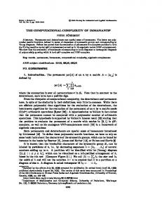
Figure 1: A database satisfying P and a corresponding database for F(P). Furthermore, for all j = 1 . . . m, we introduce the constraint {freq({d, tϕj }) ∈ [l/2, u/2]} . That is, we only measure the frequency of the formulas ϕ within the fraction of the database with d, that is, the valid truth assignments. Since exactly half of the transactions contain d, the bounds of the intervals have to be divided by 2. We denote the resulting FREQSAT-instance by F(P). It is now true that F(P) is satisfiable if and only if P is. Henceforth, we can reduce pSAT to FREQSAT. In the rest of the paperVwe will often identify the itemset I with the conjunction i∈I i. Lemma 2. P is satisfiable if and only if F(P) is satisfiable. Furthermore, ENTϕ (P) = [l, u] if and only if ENT{d,tϕ } (F(P)) = [l/2, u/2] .

Example 1. Consider the following set of extended frequency constraints P: ½ ¾ freq(a) ∈ [0.4, 0.7], freq((¬a) ∨ b) = 0.6, P = . freq(b ∧ c) ∈ [0.2, 0.4], freq(c) = 0.6 F(P) is a set of frequency constraints over the items {ta , fa , tb , fb , tc , fc , t¬a , f¬a , t(¬a)∨b , f(¬a)∨b , tb∧c , fb∧c , d, d} . The first type of constraints in F(P) make sure that tσ and fσ are complements of each other: freq({ta , fa }) = 0, freq({ta }) = 0.5, freq({fa }) = 0.5 freq({tb , fb }) = 0, freq({tb }) = 0.5, freq({fb }) = 0.5 ... freq({tb∧c , fb∧c }) = 0, freq({tb∧c }) = 0.5, freq({fb∧c }) = 0.5 The item d is in half of the transactions, and d is its complement: freq({d, d}) = 0, freq({d}) = 0.5, freq({d}) = 0.5 .

The second type of constraints makes sure that within the transactions that contain d of a satisfying database, the trues and falses are consistent: freq({d, ta , t¬a }) = 0, freq({d, t¬a , f(¬a)∨b }) = 0, freq({d, f¬a , fb , t(¬a)∨b }) = 0 freq({d, fb , tb∧c }) = 0, freq({d, ta , tb , fb∧c }) = 0

freq({d, fa , f¬a }) = 0 freq({d, tb , f(¬a)∨b }) = 0, freq({d, fc , tb∧c }) = 0,

We now express M2 by applying M1 twice, and setting the result item m equal to the union of the results of the two M1 . We can express that m is in exactly those transactions that contain either m1 or m2 as follows: freq((m ∧ ¬(m1 ∨ m2 )) ∨ ((m1 ∨ m2 ) ∧ ¬m)) = 0 We denote this expression E(m, m1 ∨ m2 ) (E of “equal”.) Let M2 (I, m) be the following expression: M1 (I, m1 ) ∪ M1 (I, m2 ) ∪ {freq(m1 ∧ m2 ) = 0, E(m, m1 ∨ m2 )} .

Finally, the third type of constraints translates the extended frequency constraints: freq({d, ta }) ∈ [0.2, 0.35], freq(d, tb∧c ) ∈ [0.1, 0.2],

freq({d, t(¬a)∨b }) = 0.3, freq({d, tc }) = 0.3

In Figure 1, two databases satisfying respectively P and F(P) have been given. The following theorem follows immediately from Lemma 2. Theorem 1. FREQSAT ≡ pSAT and hence, FREQSAT is NPcomplete.

4.2 Association Rules We can also simulate association rules in FREQSAT. An association constraint is an expression conf(I → J) ∈ [l, u], with I, J itemsets. A database D satisfies this association constraint if and only if l · freq(I, D) ≤ freq(I ∪ J, D) ≤ u · freq(I, D) .

4.2.1

Multiplication Lemma

We first introduce the following multiplication-lemma. This lemma shows how we can construct a new item m that has exactly d times the frequency of a given itemset I. Lemma 3. Let C be a set of frequency constraints, I an itemset, m an item not used in C, and d a positive integer. There exists a set of constraints Md (I, m), polynomial in the length of d, such that: (1) C ∪ {freq(I) ∈ [0, 1/d]} is satisfiable if and only if C ∪ Md (I, m) is, and (2) If D satisfies C ∪ Md (I, m), then freq({m}, D) = d · freq(I, D).

Sketch We will give extended frequency constraints with Boolean formulas that describe Md (I, J). Later on, using Lemma 2, these extended frequency constraints can be translated into regular frequency constraints. m Introduce a new item sm I . Let M1 (I, m) = {freq(sI ∨ I) = m m m 1/d, freq(sI ∨m) = 1/d, freq(sI ∧I) = 0, freq(sI ∧m) = 0}. Hence, sm I and I never occur together, and the sum of their frequencies is 1/d. Thus, freq(I) = 1/d−freq(sm I ). Similarly, freq(m) = 1/d − freq(sm I ), and hence, freq(I) = freq(m).

Hence, we can multiply frequencies by 2. By iteratively multiplying by two, we can multiply by 2k . Using the addition technique with E(·, ·), we can add frequencies. Therefore, we can multiply with an arbitrary number d. 2 Example 2. Let I be an itemset. The following expression M1 ({a}, x) forces freq({x}) to be equal to freq({a}), assuming that freq({a}) is at most 1/d: M1 (I, x)

=

{freq(sxI ∨ I) = 1/d, freq(sxI ∨ x) = 1/d, freq(sxI ∧ I) = 0, freq(sxI ∧ x) = 0}

In the rest of the construction we will often use M1 as a copying mechanism. The parameter d, however, can be different for the different expressions. Therefore we denote the value of d as a superscript to the notation; that is, we will use Md1 (I, x). M2 , M4 , and M5 are now constructed as follows: M2 (I, x2 ) =

1/5

1/5

M1 (I, x11 ) ∪ M1 (I, x21 ), ∪{freq(x11

∧

x12 )

= 0, E(x2 , x11 ∨ x21 )}

2/5

2/5

M4 (I, x4 ) =

M2 (I, x2 ) ∪ M1 ({x2 }, x12 ) ∪ M1 ({x2 }, x22 ) ∪{freq(x12 ∧ x22 ) = 0, E(x4 , x12 ∨ x22 )}

M5 (I, x5 ) =

M1 (I, x1 ) ∪ M4 (I, x4 )

1/5

∪{freq(x1 ∧ x4 ) = 0, E(x5 , x1 ∨ x4 )} The following database satisfies {freq({a}) = 0.5, freq({b}) = 0.5} ∪ M5 ({a, b}, m) . TID 1

a, b x1

2 3

a a

4 5 6 7 8 9 10

a a b b b b

4.2.2

1 sx{a,b}

Items x11 , x2

x2 x1 1 1 , s{a,b} s{a,b} 2 x 1 , x2

m x2 x1 s{x2 2 } , s{x2 2 } x12 , x4 x2 x1 s{x2 2 } , s{x2 2 } x12 , x4 x22 , x4 x22 , x4

m m m m

Reduction

Assume that besides frequency constraints C, also a set of association constraints A has been given. We show that there exists a FREQSAT-instance F(C ∪ A) that is equivalent to C ∪ A.

Reduction from C ∪ A to F(C ∪ A) An association constraint conf(I → J) ∈ [l, u] holds if and only if l · freq(I, D) ≤ freq(I ∪ J, D) ≤ u · freq(I, D) . We concentrate on l · freq(I, D) ≤ freq(I ∪ J, D); the simulation of the upper bound u is similar. Let l = α . Then, β the lower bound holds if β · freq(I ∪ J) ≥ α · freq(I). We will construct F(C ∪ A) in such a way that when it is satisfiable by a database D, only a small part of it is the encoding of a database that satisfies C ∪ A. We mark the transactions that form the database for C ∪ A, by adding a new item d to it. This gives the following constraints (we will specify the exact value of N later): freq({d}) = 1/N , and for all freq(Ij ) ∈ [lj , uj ], the constraint freq(Ij ∪ {d}) ∈ [lj /N, uj /N ]. The transactions that do not contain d can be considered as extra “workspace.” We are now ready to encode β · freq(I ∪ J) ≥ α · freq(I). We have two items mβI∪J and mα I . Using the multiplication Lemma 3, we set the frequency of mβI∪J to β times the frequency of I ∪ J: Mβ (I ∪ J, mβI∪J ) . Similarly, we set the frequency of mα I to α times the frequency of I. We can now express that β · freq(I ∪ J) ≥ α · freq(I) by requiring that evβ β α ery mα I occurs together with mI∪J : freq(¬mI∪J ∧mI ) = 0 . In this way we can translate the association constraints one by one. We have to choose N large enough, to make sure that there is enough workspace to do the multiplications. Hence, N should be at least α, where α is the greatest denominator of a bound of an association constraint. We denote this number NA . This gives us the set of extended frequency constraints P(C ∪ A). Since we used arbitrary Boolean formulas in the translation, we still need to apply the translation from extended frequency constraints to regular frequency constraints. We call the resulting set of constraints F(C ∪ A). Theorem 2. C ∪A is satisfiable if and only if F(C ∪A) is satisfiable. Furthermore, ENTI (C ∪ A) = [l, u] if and only if ENTI (F(C ∪ A)) = [l/(2 · NA ), u/(2 · NA )]. Example 3. Let C ∪ A be the following set: {freq(a) = 3/4, freq({a, b}) = 1/2}∪{conf(a → b) ∈ [1/2, 1]} . NA equals 2. The following databases satisfy respectively C ∪ A and P(C ∪ A):

TID Items 1 a 2 a, b 3 a, b 4 b

−→

TID 1 2 3 4 5 6 7 8

d, a d, a, b d, a, b d, b

Items m1a , m2a , m1a , m2a , m1a , m2a , m2a , m2a m2a

m2{a,b} m2{a,b} m2{a,b} m2{a,b}

Entailment problems. Consider the following three entailment problems associated with FREQSAT:

(1) FREQENT(C, freq(I) ∈ [l, u]) Decide whether C |= freq(I) ∈ [l, u]. (2) T-FREQENT(C, freq(I) ∈ [l, u]) Decide whether C |=tight freq(I) ∈ [l, u]. (3) Func T-FREQENT(C, I) Give [l, u] such that C |=tight freq(I) ∈ [l, u]. The complexity of these three problems is related to the complexity of FREQSAT. Since we can use association rules, the entailment problems are equivalent with the entailment problems in the context of conditional events studied by Lukasiewicz in [11]. Hence, we obtain the following theorem:

• • •

Theorem 3. FREQENT is co − NP-complete. T-FREQENT is DP-complete. Func T-FREQENT is FPNP -complete.

4.3

Axiomatization

We show that FREQSAT is not finitely axiomatizable. We first give a lemma and theorem that provide a set of axioms that are sound and complete in the special case of sets of frequency constraints that contain an expression freq(I) = fI for all sets I ⊆ I. The number of axioms depends on the set I, and the axioms are only complete in this very special case. In Theorem 4, we then show that in general, no finite axiomatization of FREQSAT exists.

Lemma 4. Let f and g be two functions defined on the subsets of a finite set I. The following two expressions are equivalent: (1) For all I ⊆ I, f (I) = (2) For all J ⊆ I, g(I) =

P

I⊆K

P

g(K);

I⊆K (−1)

|K−I|

f (K).

Theorem 4. Let for all I ⊆ I, fI be a rational number. There exists a transaction database D such that for all I ⊆ I, freq(I, D) = fI if and only if, for all I ⊆ I, the following rule holds: X RI (I) σI (I) = (−1)|K−I| fK ≥ 0 I⊆K⊆I

Proof. If Let d be the least common multiplier of the denominators of the sums σI (I). The database D consists of the following transactions: for every set I ⊆ I, there are d · σI (I) transactions (tid, I). Notice that all d · σI (I) are positive integers. Thus, for all I ⊆ I, freq(I, D) = P I⊆J σI (J). Using Lemma 4, we hence get freq(I, D) = fI . Only If Let D be a database that fulfills the given frequencies. Let φI denote the fraction Pof transactions (tid, J), with J = I. Hence, freq(I, D) = I⊆K φK . Via Lemma 4, we get that σI (I) equals φI . Hence, since all φI must be positive, all σI (I) must be as well.

Theorem 5. Every axiomatization for FREQSAT that does not include an axiom that involves the frequency of all nonempty itemsets is incomplete. Therefore, FREQSAT is not finitely axiomatizable.

Sketch Let n be an arbitrary number. We can construct a FREQSAT problem C over the set I = {i1 , . . . , in }, such that (a) C is not satisfiable, but, (b) every strict subset of C is satisfiable. Furthermore, C contains one expression freq(I) = fI for every I ⊆ I. From (a) and (b) it follows then that an axiomatization for FREQSAT must contain at least one axiom that involves every frequency constraint in the input. Indeed; suppose that the axioms A1 , A2 , . . . , Am are sound and complete for FREQSAT, but none of the axioms Ai involves all frequencies. Because C is not satisfiable, there must be at least one axiom A that is not satisfied by C. This is so because C contains an expression freq(I) = fI , for every subset I of I. Hence, every expression freq(I) ∈ [l, u] entailed by C is either in contradiction with freq(I) = fi , or is less expressive. Therefore, if it can be derived by the axioms that C is not satisfiable, then this can be derived in one step. Suppose that this unsatisfied axiom A does not involve itemset I, and c is the constraint in C involving I. Then we have the following contradiction: C \ {c} is satisfiable, but violates A.

Lemma 5. Let J be a finite set of items, n = |J |, k is an integer with 1 ≤ k ≤ n. Let D be a transaction database that satisfies the following collection Ck [J ] of frequency expressions: ! Ã ! Ã n−1 . n ∀j ∈ J : freq({j}) = k k−1 ! Ã ! Ã n−2 . n ∀j1 6= j2 ∈ J : freq({j1 , j2 }) = k k−2 Then, for all transactions (tid, J) in D, the number of items in J ∩ J equals k.

Sketch Let for all i = 0 . . . n, δi =def |{(tid, I) ∈ D | |J ∩ I| = i}| . Pn It is clear that |D| = i=1 δi . Let X Si =def supp(I, D) . I⊆J ,|I|=i

Hence, since D satisfies Ck [J ], S0

We assume that n is even. (a similar system can be found for n odd) Let C be ¯ ) ( ¯ [ 2(n−|I|) ¯ {freq(I) = 0} freq(I) = n ¯∅⊂I⊂I (2 ) − 1 ¯ This set C fulfils the conditions (a) and (b). For all I 6= ∅, we have: σI (I) =

X

(−1)|K−I|

I⊆K⊂I

=

σI (∅)

=

K⊂I

Thus, C is not satisfiable. However, for every nonempty set I, if we remove the expression with I from C, the resulting system C 0 is satisfiable. Let I be odd: C 0 ∪ {freq(I) = 2(n−|I|) −1 } is satisfiable, if I 6= I is even, C 0 ∪ {freq(I) = (2n ) 2(n−|I|) +1 } (2n )

is satisfiable, and for I = I, C 0 ∪{freq(I) = (21n ) } is satisfiable. These claims can easily be proved by checking the changes in the sums σI (I) given above. 2

5. FREQSAT{LTRANS} In this section we show that knowing an upper bound on the length of the transactions does not affect the complexity of the FREQSAT-problem. Moreover, for any subset C of {ntrans, ndup}, FREQSAT({ltrans} ∪ C) is equivalent to FREQSAT(C).

=

! Ã ! Ã !Ã n−2 . n n |D| k k−2 2

S0 S2

= =

n X

i=1 n X

δi ,

n X

S1 =

iδi

i=1

i(i − 1)δi /2

i=1

These last equalities in combination with

(n−|K|)

2 1 = − n (2n ) − 1 (2 ) − 1

S1 = |D| · n ·

Every transaction of length i has i subsets of length 1, and i(i − 1)/2 subsets of length 2. So, it is also true that

1 (1 − (−1)n−|I| ) (2n ) − 1

(−1)|K|

|D|,

! Ã ! n−1 . n k k−1

Thus, k(k − 1)S0 = (k − 1)S1 = 2S2 .

2(n−|K|) (2n ) − 1

Hence, for all I 6= ∅, σI I equals 0 if |I| is even, and 2 if |I| is odd. For I = ∅, we get: X

S2

=

Ã

k(k − 1)S0 = (k − 1)S1 = 2S2 , lead to 0 = kS0 − S1 0 = (k − 1)S1 − 2S2

= =

n X

i=1 n X

(k − i)δi i(k − i)δi

i=1

From this it can be shown that for all i 6= k, δi = 0.

2

For every δ, the set of constraints Ck [J ] is satisfied by the database Dk,δ that consists of δ transactions (tid, J), for all J ⊆ J of length k. Hence, every database D with all transactions having length exactly k, can be embedded in the database Dk,|D| . The next definition and theorem are based on this observation. Again an item d, not in J is used to mark the transactions that identify the embedding of D.

Definition 1. Let C be the following set of frequency constraints: C = {freq(I1 ) ∈ [l1 , u1 ], . . . , freq(Im ) ∈ [lm , um ]} . S Let J = m j=1 Ij , n = |J |, 1 ≤ k ≤ n, and let d be an item not in J . ( à !) . n λk (C) =def freq({d}) = 1 ∪ Ck [J ] ∪ k à !#) à ! ( " m . n . n [ , uj freq({d} ∪ Ij ) ∈ lj k k j=1 Example 4. The following databases satisfy respectively C and λ2 (C) for C = {freq({a, b}) = 0.5, freq({b, c}) ∈ [0.4, 0.6]} .

TID 1 2

Items a, b b, c

−→

TID 1 2 3 4 5 6

Items a, b d a, b a, c a, c b, c d b, c

Theorem 6. A set C of frequency constraints is satisfiable by a database with all transactions of constant length k if and only if λk (C) is in FREQSAT. Proof. Let C be {freq(I1 ) ∈ [l1 , u1 ], . . . , freq(Im ) ∈ [lm , um ]} , S and let J be the set of items m j=1 Ij .

If : Suppose that D satisfies λk (C). Let D d be the following database:

Dd =def {(tid, J) | (tid, J ∪ {d}) ∈ D} ¡ ¢ The number of transactions in D d is |D|/ nk , and the numd ber¡ of¢ transactions in |D| · ¢ that contain Ij lays between ¡nD n lj / k and |D| · uj / k . Hence, its frequency in D d is between lj and uj . Therefore, D d satisfies C. Furthermore, because D satisfies Ck [J ], Lemma 5 states that every transaction in D contains exactly k items from J . Henceforth, all transactions in D d have length k (d is not in J ). Only If : Suppose that D is a database with all transactions of length¡ k¢ that satisfies C. We construct a database D 0 with |D| nk transactions that satisfy λk (C). For every subset I of size k of J , there will be supp(I, D) transactions (tid, I ∪ {d}), and |D| − supp(I, D) transactions (tid, I) in D0 . Thus, the absolute number of transactions containing I ∪ {d} in D 0 is the same as the absolute ¡ ¢ number of transactions containing I in D, but |D 0 | is nk times larger than |D|. ¡ ¢ Hence, the frequency of Ij ∪{d} in D 0 equals freq(Ij , D)/ nk . ¡ n¢ ¡ n¢ The frequency of d is |D|/(|D| · k ) = 1/ k . It also holds that D 0 satisfies Ck [J ]; the projection of D 0 on J consists of |D| copies of I, for every subset I of J of size k.

Corollary 1. For all C ⊆ {ntrans, ndup}, FREQSAT({ltrans} ∪ C) ≡ FREQSAT(C) . Sketch Let C = {freq(Ij ) ∈ [lj , uj ] S | j = 1 . . . m} be a set of frequency constraints, and let I = n j=1 Ij , |I| = n. FREQSAT({ltrans} ∪ C) ≥ FREQSAT(C): the number of items is an upper bound for transaction length, and hence, (C, v1 , . . . , vk ) is in FREQSAT{c1 , . . . , ck } if and only if (C, n, v1 , . . . , vk ) is in FREQSAT{ltrans, c1 , . . . , ck }.

FREQSAT({ltrans} ∪ C) ≤ FREQSAT(C): the proof of this direction is based on Lemma 5. Let C be a set of frequency constraints. Assume that C is satisfiable by a transaction database D, and D has a maximal transaction size of n. Since Lemma 5 only holds for transaction databases of length exactly lt, we need to add extra items to compensate for transactions that are too short. When C includes ndup, some care is required to avoid that the new items change the number of duplicates. 2

6.

FREQSAT{NTRANS} In the last section we saw that knowing a maximal transaction length does not add expressive power to FREQSAT. For the number of transactions ntrans, the question whether it adds to the complexity is open. We show that FREQSAT reduces to FREQSAT{ntrans}, and that FREQSAT{ntrans} is equivalent to Intersection Pattern Problem (IP) [8] w.r.t. computational complexity. IP is the following problem: given an n × n matrix C with integer entries, do there exist sets S1 , . . . , Sn such that |Si ∩ Sj | = C[i, j]? If such sets exist, C is called an intersection pattern. In [8], it is claimed that IP is NP-complete. However, the inclusion in NP has only been proven for the case the entries in the matrix C are bounded by a fixed constant [7]. For the general problem, the inclusion of IP in NP is still open. For the entailment, we show that, unlike for FREQSAT, the set ENTn I (C) = {freq(I, D) | D |= C, |D| ≤ n}, is no longer an interval of the rational numbers. This is of course hardly surprising, since the frequencies in a database with at most n transactions can only be of the form pq , with 0 ≤ p ≤ n, and 1 ≤ q ≤ n. Therefore, it would be more fair to ask the following question: if pq1 , pq2 ∈ ENTn I (C), is it true that for every p with p1 ≤ p ≤ p2 , also pq ∈ ENTn I (C)? We will answer this question negatively. Moreover, given an arbitrary set R = {r1 , . . . , rk } of rational numbers, we will show that there exists a set of constraints C, an itemset I, and a positive integer n, all having description size polynomial in the size of R, such that ENTn I (C) = R. This shows that the properties of the FREQSAT-problem change fundamentally if we restrict the number of transactions.

6.1

Relation with FREQSAT

Theorem 7. FREQSAT ≤ FREQSAT{ntrans}

Proof. Given a FREQSAT-problem C, by Lemma 1, there exists an upper bound nC (with size polynomial in C), such that if C is satisfiable, then C is satisfiable by a database of size maximally nC . Hence, C is in FREQSAT if and only if (C, nC ) is in FREQSAT{ntrans}.

6.2 INTERSECTION PATTERN We show that IP is equivalent to FREQSAT{ntrans}.

6.2.1 Reduction From IP to FREQSAT{ntrans} It is clear that IP can be reduced to FREQSAT{ntrans}; if an n × n matrix C is an intersection pattern, Snthen there exists a realization P S1 , . . . , Sn of C such that | i=1 Si | is at most N (C) = 1≤i≤n C[i, i]. Every instance of IP can now be reduced to the an instance of FREQSAT{ntrans} as follows. The upper bound on the number of transactions is set to N (C). We make sure that the number of transactions in a satisfying database is exactly N (C) by adding the following constraint (e is a new item): freq({e}) = 1/N (C). We furthermore have items s1 , . . . , sn . For every 1 ≤ i, j ≤ n, the constraint freq({si , sj }) = C[i, j]/N (C) is added. If D is a satisfying database, then the sets Si = {tid | (tid, J) ∈ D, si ∈ J}, for i = 1 . . . n form a realization of C, and vice versa. ¶ 2 1 . The following sets 1 1 form a realization of C: S1 = {1, 2}, S2 = {1}. The corresponding FREQSAT{ntrans}-problem is (C, 3) with ¾ ½ freq({e}) = 1/3, freq({s1 }) = 2/3, . C= freq({s2 }) = 1/3, freq({s1 , s2 }) = 1/3 Example 5. Let C =

µ

The satisfying database of C that corresponds with the realization S1 = {1, 2}, S2 = {1} is:

D =

TID Items 1 s 1 , s2 2 s1 3

6.2.2 Reduction From FREQSAT{ntrans} to IP We give a non-deterministic polynomial many-one reduction from FREQSAT{ntrans} to IP. Such a reduction shows that if IP is in NP, then so is FREQSAT{ntrans}. We only illustrate the reduction with an example. Let (C, nt) be an instance of the FREQSAT{ntrans} problem. The first step in the reduction is to reduce the cardinalities of the sets in the input to 2. For example; a constraint freq({a, b, c, d}) ∈ [0.1, 0.3] in C, must be replaced with a number of constraints that only involve itemsets of cardinality at most 2. This would be easy if we knew the frequencies of the prefixes of {a, b, c, d}. Indeed; suppose that we know that freq({a}) = 0.5, freq({a, b}) = 0.3, freq({a, b, c}) = 0.2, and freq({a, b, c, d}) = 0.1. Then we could introduce new items i{a,b} , i{a,b,c} , and i{a,b,c,d} . These items replace respectively {a, b}, {a, b, c}, and {a, b, c, d}. We enforce these semantics as follows: freq({i{a,b} }) = 0.3, freq({i{a,b} , a}) = 0.3, freq({i{a,b} , b}) = 0.3, freq({a, b}) = 0.3 freq({i{a,b,c} }) = 0.2, freq({i{a,b,c} , i{a,b} }) = 0.2, freq({i{a,b,c} , c}) = 0.2, freq({i{a,b} , c}) = 0.2 freq({i{a,b,c,d} }) = 0.1, freq({i{a,b,c,d} , i{a,b,c} }) = 0.1, freq({i{a,b,c,d} , d}) = 0.1, freq({i{a,b,c} , d}) = 0.1 In this way, we can replace itemsets of high cardinality by a chain of sets of cardinality at most 2. Of course, in general, we do not know the exact frequencies of the prefixes of the

sets that are too long. Therefore, in the non-deterministic polynomial many-one reduction, we start by guessing them. If C has a solution, then there exists a correct guess. In the second step, we have to encode the FREQSAT{ntrans}problem as a matrix C. We can at this point assume that C only contains itemsets of cardinality at most 2, and that the frequencies are given exactly (that is, no intervals). We guess the total number of transactions n, under the constraint 0 ≤ n ≤ nt. In the matrix C, every row and column corresponds to one item. The entry C[i, j] that corresponds to the item i and the item j is filled as follows: if there is an expression freq({i, j}) = f in C, then C[i, j] = f ·n. Else, the entry C[i, j] is filled randomly by a number between 0 and n. If in the end, one of the entries in C is not an integer, we reject, since one of the guesses was wrong. In the other case, an instance for IP has been constructed. There exists a series of guesses that leads to an intersection pattern C if and only if the original problem (C, nt) is in FREQSAT{ntrans}.

6.3

Entailment

Lemma 2 can be extended to FREQSAT{ntrans}; that is, we can extend FREQSAT{ntrans} to arbitrary Boolean formulas. We assume that the maximal number of transactions is set to nt. Consider the following set of expressions over the items a, b, c: freq({i}) = 1/nt freq({a, b}) = 0 freq({a, c}) = 0 freq({b, c}) = 0 freq(a ∨ c) = k/nt freq(b ∨ c) = k/nt The first constraint makes sure that there are exactly nt transactions. The next three constraints enforce that the transactions with a, the ones with b, and the ones with c are disjoint. Let A be the set of transactions with a, B the ones with b, and C the ones with c. The last two constraints express that |A∪C| = |B∪C| = k/nt. Let’s now consider the set ENTnt a∨b (C). Suppose that C contains l items, 0 ≤ l ≤ k. Then, both A and B contain k − l transactions, and hence, 2·l |A ∪ B| = 2(k − l). Therefore, ENTnt a∨b (C) = { nt | l = nt 0 . . . k}. Thus, 0/nt, 2/nt ∈ ENTa∨b (C), but 1/nt is not in ENTnt a∨b (C). We now show that we can express every arbitrary set. Let R = {r1 , . . . , rk } be a set of positive rational numbers between 0 and 1. First, we equalize the denominators, that is, let R = { pq1 , . . . , pqk }. We set the number of transactions to q. We make sure that the number of transactions is exactly q, by adding the constraint freq({i}) = 1/q . ci and ni are new items that are introduced for the construction. We construct a set of constraints such that freq({ni }) is either 0 or pi /q. The expression will be such that freq({ni }) = pi /q, if and only if freq({ci }) = 0. Hence, ci acts as some sort of switch; if ci is “on”, freq(ni ) will be 0. We will make sure in the construction that only one of the switches is “off.” Let di be a new item. We first make a construction such that freq(di ) is 1/q if freq(ci ) is 0 and vice versa: freq(ci ∨ di ) = 1/q, freq(ci ∧ di ) = 0 Then we use the multiplication lemma to express that the frequency of ni is pi times the frequency of di : Mpi (di , ni ) .

We set a target item t to n1 ∨. . .∨nk : E(t, n1 ∨. . .∨nk ). We still have to make sure that only one of the ni ’s is non-zero. Remember that ni was non-zero if and only if ci was zero. Hence, we add freq(c1 ∨ . . . ∨ ck ) = (k − 1)/q Thus, exactly k − 1 of the frequencies of c1 , . . . , ck are 1/q, and therefore, for exactly one i, freq(ci ) = 0. Let E be the set of constraints we just constructed. It is now true that ENTqt (E) = R.

7.1 FREQSAT{ndup=1} Let C be a set of constraints, and nd be a positive integer. Let the binary representation of nd be Bl . . . B0 . We introduce l + 1 new items, b0 , . . . , bl . We use the bj ’s to eliminate duplicates. That is, nd + 1 transactions with set of items I, will be replaced by transactions with set of items: I, I ∪{b0 }, I ∪ {b1 }, I ∪ {b0 , b1 }, . . . , I ∪ {bj | Bj = 1}. Let I ∪ B be an itemset, I ∩ B = ∅, and bj ∈ (B ∪ I) → bj ∈ B. ν(I ∪ B) is the number associated with I; that is: X j 2 . ν(I ∪ B) = bj ∈B

Example 6. Consider the set R = {1/2, 1/3, 1/4}. First we equalize the denominators: R = {6/12, 4/12, 3/12} . We set the upper bound on the number of transactions to 12. We make sure that there are exactly 12 transactions by adding the constraint

We have to make sure that the numbers of the transactions are never higher than nd. This can be done as follows: for all ` such that B` = 0, add the constraint freq({bj | Bj = 1, j > `}∪{b` }) = 0. Let Bnd be the set of these constraints. ∆nd (C) =def C ∪ Bnd−1 . It is now true that (C, nt, nd) is in FREQSAT{ntrans, ndup}, if and only if (∆nd (C), nt) is in FREQSAT{ntrans, ndup = 1}.

freq({i}) = 1/12 . New items c1 , c2 , c3 , and d1 , d2 , d3 are introduced. We add the following constraints to ensure that freq(dj ) = 1/12 if and only if freq(cj ) = 0. Otherwise freq(dj ) = 0. freq(c1 ∨ d1 ) = 1/12, freq(c1 ∧ d1 ) = 0 freq(c2 ∨ d2 ) = 1/12, freq(c2 ∧ d2 ) = 0 freq(c3 ∨ d3 ) = 1/12, freq(c3 ∧ d3 ) = 0 Next, the items n1 , n2 , n3 are introduced that have a frequency of respectively 3·freq(d1 ), 4·freq(d2 ), and 6·freq(d3 ): M3 (d1 , n1 ), M4 (d2 , n2 ), M6 (d3 , n3 ) We make sure that exactly 2 of c1 , c2 , c3 are non-zero: freq(c1 ∨ c2 ∨ c3 ) = 2/12 . Hence, exactly one of freq(cj ) is 0, and thus, exactly one of freq(dj ) is 1/12, the other are 0. Therefore, either freq(n1 ) = 3/12, freq(n2 ) = 0, freq(n3 ) = 0, or freq(n1 ) = 0, freq(n2 ) = 4/12, freq(n3 ) = 0, or freq(n1 ) = 0, freq(n2 ) = 0, freq(n3 ) = 6/12. Finally, the item t is set to equal n1 ∨ n2 ∨ n3 :

Example 7. The binary representation of 10 is 1010. Hence, B10 is the following set of constraints: {freq({b3 , b2 }) = 0, freq({b3 , b1 , b0 }) = 0} . Every database that satisfies these constraints can have transactions (tid, J) with J ∩ {b0 , b1 , b2 , b3 } equal to: {}, {b0 }, {b1 }, {b0 , b1 }, {b2 }, {b0 , b2 }, {b1 , b2 } {b0 , b1 , b2 }, {b3 }, {b0 , b3 }, {b1 , b3 } These transactions have respectively as associated numbers 0, . . . , 10. The constraints in B10 disallow transactions that contain {b3 , b1 , b0 }, {b3 , b2 }, {b3 , b2 , b0 }, {b3 , b2 , b1 }, {b3 , b2 , b1 , b0 } . These transactions have respectively as associated numbers 11, . . . , 15. Therefore, adding the items b0 , . . . , b3 , and B10 makes it possible to reduce the number of duplicates with a factor 11. Theorem 8. FREQSAT{ndup} ≡ FREQSAT{ntrans, ndup} FREQSAT{ntrans} ≤ FREQSAT{ndup}

E(t, n1 ∨ n2 ∨ n3 ) The set of frequencies for t entailed by this set of constraints equals {3/12, 4/12, 6/12}.

7. FREQSAT{NDUP} In this section we study FREQSAT{ndup}. First we show that we can always reduce a FREQSAT{ndup}-instance (C, nd) to an instance (C 0 , 1). Hence, we show that the following problem: given C, decide whether (C, 1) is in FREQSAT{ndup}, is equivalent to FREQSAT{ndup}. We denote this problem FREQSAT{ndup = 1}. We show that FREQSAT{ntrans} reduces to FREQSAT{ndup}. We also show that FREQSAT{ndup = 1} is PP-hard. Hence, knowing the number of duplicates does add complexity to the FREQSAT-problem.

Proof. FREQSAT{ndup} ≤ FREQSAT{ntrans, ndup}: With n items and nd duplicates, one can have maximally nd · 2n transactions. Hence, (C, nd) ∈ FREQSAT{ndup} if and only if (C, nd · 2n , nd) ∈ FREQSAT{ntrans, ndup}. FREQSAT{ndup = 1} ≥ FREQSAT{ntrans, ndup S = 1}: Let C = {freq(Ij ) ∈ [lj , uj ], j = 1 . . . m}, I = j=1m Ij . Let bl . . . b0 be the binary representation of nt. (C, nt) ∈ FREQSAT{ntrans, ndup = 1} if and only if {freq({d} ∪ Ij ) ∈ [lj /2, uj /2], j = 1 . . . m} ∪ {freq({d}) = 0.5, freq(d) = 0.5, freq(d, d) = 0} ∪ Bnt−1 ∪ {freq({bj , d}) = 0, j = 1 . . . l} ∪ {freq({i, d}) = 0 | i ∈ I} is in FREQSAT{ndup = 1}. In this reduction, the simulating database is split into two equally sized parts. The actual

database consists of the transactions containing d. In the other part, every transaction contains d and some items of {b0 , . . . , bl }. Since Bnt−1 holds, and the number of duplicates is 1, the d-part has maximally nt transactions. Because both parts have equal size, the actual database, that is embedded as the d-part, contains maximally nt transactions as well. FREQSAT{ndup} ≥ FREQSAT{ntrans}: (C, nt) is in FREQSAT{ntrans} if and only if (C, nt, nt) is in FREQSAT{ntrans, ndup}. Theorem 9. FREQSAT{ndup = 1} is in PSPACE Proof. S Let C = {freq(Ij ) ∈ [lj , uj ], j = 1 . . . m}, and let I = m j=1 Ij . Every database D that satisfies C, and with ndup(D) ≤ 1, has at most 2|I| transactions. We show a non-deterministic procedure to decide the satisfiability of C that uses at most polynomial space in the length of C. In this way we show that FREQSAT{ndup = 1} is in NPSPACE, and thus by Savitch’s Theorem [15, p. 149-150], also in PSPACE. We “guess” a database D, transaction by transaction. We avoid generating the same transaction twice, by requiring that every new transaction comes lexicographically strictly after the previous one. During database generation, we maintain m counters for I1 , . . . , Im , and 1 counter for |D|. For every new transaction (tid, J), we increment the counter |D|, and we do the checks Ij ⊆ J. For all j such that Ij ⊆ J, the counter for Ij is incremented. After at most 2|I| guesses, we stop the database generation. We then check whether Counter(Ij )/Counter(|D|) is within the interval [lj , uj ]. If this is the case for all j = 1 . . . m, we accept, otherwise, we reject.

7.2 FREQSAT{ndup} is PP-hard Theorem 10. FREQSAT{ndup} is PP-hard. Sketch We reduce MAJSAT to FREQSAT{ntrans, ndup = 1}. Let ϕ be the given formula with variables x1 , . . . , xn . We construct a set of constraints C, such that (C, 2n+1 ) is in FREQSAT{ntrans, ndup = 1} if and only if more than half of the truth assignments to ϕ are accepting. This reduction is very similar to the reduction of pSAT to FREQSAT. In FREQSAT{ntrans, ndup = 1} we can furthermore make sure that every transactions represents a different truth assignment, and that the total number of truth assignments is 2n . Hence, the frequency of a certain itemset {d, tσ } corresponds directly to the number of satisfying truth assignments. The requirement that ϕ is true in more than half of the truth assignments can thus be stated as follows: freq({tϕ , d}) ∈ [(2n−1 + 1)/2n+1 , 1] , since 2n transactions represent valid truth assignments (the ones that contain d), and hence “more than half” is the same as “at least (2n−1 + 1).” 2

7.3

Entailment

Notice that the construction in the proof of the PP-hardness of FREQSAT{ndup = 1}, has direct repercussions for the study of the complexity of the following function problem, named FuncFREQENT{ndup = 1}. Problem FuncFREQENT{ndup = 1}: Input: A pair (C, I), with C a finite set of expressions C = {Ij ∈ [lj , uj ] | j = 1 . . . m} Output: Let S = {freq(I, D) | D |= C, ndup(D) = 1}. If C is satisfiable, the interval [min(S), max(S)]. Else, if C is not satisfiable, no. 2 Theorem 11. FuncFREQENT{ndup} is #P-hard. Proof. Let ϕ be an arbitrary Boolean formula. Construct C as in the proof of Theorem 10. Let now C 0 be the constructed C minus the constraint freq({tϕ , d}) ∈ [(2n−1 + 1)/2n+1 , 1]. Let [l, u] be output of the FuncFREQENT{ndup = 1}-problem (C, {d, tϕ }). Via a similar reasoning as in the proof of Theorem 10, we get that l and u both equal the number of satisfying assignments of ϕ, divided by 2n+1 . Hence, 2n+1 · l is the solution of the #SAT-problem with input ϕ.

8.

APPLICATIONS

Privacy Data Mining can be a serious threat to the privacy. Therefore, methods are developed to adapt databases in such a way that still meaningful data mining results can be produced from it, but the privacy of the individual data are not compromised [2]. It is, however, conceivable that the mining is done by a trusted party. In that case, there is no risk of disclosure based on the original data. Even though, the results of the mining themselves can disclose more of the original data than is desirable. The process of trying to reconstruct parts of the original database from data mining results is called inverse data mining [13]. The FREQSATproblem, its various variants and the entailment problems can be situated in this context. The results of a frequent set mining operation can be represented as an instance of FREQSAT. Inverse data mining would then amount to deriving the frequencies of other itemsets, not in the result set. In this context, the high complexities of the problems studied in this paper are bad news: suppose that we want to publish some itemsets with their frequencies, but first we want to assess how much these frequencies disclose of the original dataset. This problem can be stated as one of the variants of FREQSAT. The high complexity of the FREQSAT-problems in this paper, however, show that there is little hope that it is effectively possible to assess the degree of disclosure. On the bright side, the high complexity means also that it is potentially very hard to break the privacy. However, the situation is different from that of, for example, public key encryption. In inverse mining, partial information can be derived with incomplete methods, whereas, in general, in public key encryption, the code cannot be partially broken. Hence, in inverse mining, the more computing power one has, the more one can be derived. Therefore, unless one has superior computing power over potentially malicious parties, the results of mining cannot be guaranteed to be safe.

Condensed Representations Another application is making condensed representations [12] of frequent itemsets. In such condensed representations typically only non-redundant information is stored. Entailment of frequencies as in the FREQSAT-problem allows for derivation of frequencies. The stronger the deduction mechanism, the more redundancy in the set of frequencies can be found. The complexity results in this paper indicate that complete deduction in the most general context is infeasible, and hence, incomplete, yet tractable methods are more appropriate. Frequent Itemset Mining Algorithms A third application is improving the pruning of frequent itemset mining algorithms. All frequent set mining algorithms use the monotonicity rule to prune substantial parts of the search space. This monotonicity rule can be seen as a very simple example of deduction. Based on partial frequency information of some itemsets, bounds on the frequencies of yet to be counted sets are derived. If these bounds establish that a certain set must be certainly frequent or certainly infrequent, the counting of it can be omitted in some cases. In the context of FREQSAT, frequency constraints can be used to model the frequency information gathered in previous scans over the database. The deduction can then be used to identify sets that are certainly frequent/infrequent. In [3, 4, 6], in some form, deduction rules are used in order to improve pruning and speed up frequent set mining algorithms.

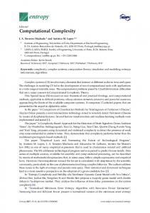
9. SUMMARY AND CONCLUSION The complexity of the FREQSAT-problem and its variants was studied. The following hierarchy illustrates the relations: PSPACE

FREQSAT{ndup}

FREQSAT{ltrans,ndup}

FREQSAT{ntrans,ndup}

FREQSAT{ltrans,ntrans,ndup}

PP

FREQSAT{ntrans}

NP

FREQSAT

FREQSAT{ltrans,ntrans}

IP

FREQSAT{ltrans}

FREQSAT was shown to be NP-complete. It was also shown that the extensions to arbitrary formulas and to association rules do not add extra expressive power to FREQSAT.

The exact complexity is unknown. Assuming that NP 6= PP, FREQSAT{ndup} is provably harder than FREQSAT. This very high complexity is bad news from a privacy point of view; it states that it is almost impossible to assess how much some itemsets with their frequencies reveal from the underlying database. The main question left open in this paper is what the exact complexities of FREQSAT{ntrans} and FREQSAT{ndup} are.

10.

REFERENCES

[1] R. Agrawal, T. Imilienski, and A. Swami. Mining association rules between sets of items in large databases. In Proc. ACM SIGMOD, pages 207–216, 1993.

[2] R. Agrawal, and R. Srikant. Privacy-preserving data mining. In Proc. ACM SIGMOD, pages 439–450, 2000. [3] Y. Bastide, R. Taouil, N. Pasquier, G. Stumme, and L. Lakhal. Mining frequent patterns with counting inference. SIGKDD Explorations, 2(2):66–75, 2000. [4] R. J. Bayardo. Efficiently mining long patterns from databases. In Proc. ACM SIGMOD, pages 85–93, 1998. [5] T. Calders. Deducing bounds on the support of itemsets. In Database Support for Data Mining Applications, LNCS 2682, Springer, to appear 2004. [6] T. Calders and B. Goethals. Mining all non-derivable frequent itemsets. In Proc. PKDD Int. Conf. Principles of Data Mining and Knowledge Discovery, pages 74–85. Springer, 2002. [7] V. Chv´ atal. Recognizing intersection patterns. Annals of Discrete Mathematics - Combinatorics 79, 8(I):249–251, 1980. [8] M.R. Garey and D.S. Johnson. Computers and Intractability: A Guide to the Theory of NP-completeness. Freeman, New York, 1979. [9] G. Georgakopoulos, D. Kavvadias, and C. H. Papadimitriou. Probabilistic satisfiability. Journal of Complexity, 4:1–11, 1988. [10] J. Hipp, U. G¨ untzer, and G. Nakhaeizadeh. Algorithms for association rule mining - a general survey and comparison. SIGKDD Explorations, 2(1):58–64, 2000. [11] T. Lukasiewicz. Probabilistic logic programming with conditional constraints. ACM Transactions on Computational Logic, 2(3):289–339, 2001.

The complexity of FREQSAT{ntrans} is still an open question. We proved that FREQSAT{ntrans} is NP-complete if IP is in NP. We also illustrated that FREQSAT{ntrans} has different properties than FREQSAT by showing that the set ENTnt I (C) can be any set of rational numbers, whereas in FREQSAT, this set is always an interval of the rational numbers. This can be an indication that the complexity of FREQSAT{ntrans} is higher than the complexity of FREQSAT, since the linear programming techniques that can be used for FREQSAT and pSAT cannot be used for FREQSAT{ntrans}.

[14] N. Nilsson. Probabilistic logic. Artificial Intelligence, 28:71–87, 1986.

FREQSAT{ndup} is the most complex of the different variants of FREQSAT. Its complexity is between PP and PSPACE.

[15] C.H. Papadimitriou. Computational Complexity. Addison-Wesley, 1994.

[12] H. Mannila and H. Toivonen. Multiple uses of frequent sets and condensed representations. In Proc. KDD Int. Conf. Knowledge Discovery in Databases, 1996. [13] T. Mielik¨ ainen. On inverse frequent set mining. In Workshop on Privacy Preserving Data Mining, 2003.