Apr 8, 2011 - simulations for an idealized 2:1 model molten salt. In agreement ... than network-forming compounds to the simple ionic liquid picture, are ...
ARTICLE pubs.acs.org/JPCB
Computational Verification of Two Universal Relations for Simple Ionic Liquids. Kinetic Properties of a Model 2:1 Molten Salt J. A. Armstrong and P. Ballone* School of Mathematics and Physics, Queen’s University Belfast, Belfast BT7 1NN, U.K. ABSTRACT: Two semianalytical relations [Nature, 1996, 381, 137 and Phys. Rev. Lett. 2001, 87, 245901] predicting dynamical coefficients of simple liquids on the basis of structural properties have been tested by extensive molecular dynamics simulations for an idealized 2:1 model molten salt. In agreement with previous simulation studies, our results support the validity of the relation expressing the self-diffusion coefficient as a function of the radial distribution functions for all thermodynamic conditions such that the system is in the ionic (ie., fully dissociated) liquid state. Deviations are apparent for highdensity samples in the amorphous state and in the low-density, low-temperature range, when ions condense into AB2 molecules. A similar relation predicting the ionic conductivity is only partially validated by our data. The simulation results, covering 210 distinct thermodynamic states, represent an extended database to tune and validate semianalytical theories of dynamical properties and provide a baseline for the interpretation of properties of more complex systems such as the roomtemperature ionic liquids.
1. INTRODUCTION The physics of simple liquids has achieved a remarkable degree of success in describing equilibrium properties of fluid systems made of spherical particles interacting via pair potentials.1 Semianalytical theories based on integral equations, in particular, predict thermodynamic functions and the equilibrium structure of neutral and charged homogeneous fluids at a very modest computational cost, requiring only a few minutes on a desktop computer. In most cases, the same quantities can be computed at better than ∼1% accuracy by molecular dynamics (MD) and Monte Carlo simulations with an effort that is still modest on the scale of present-days ab initio studies. The same bright picture, however, does not include dynamical and nonequilibrium aspects, and even linear dynamic coefficient such as diffusion and viscosity coefficients, or, for ionic liquids, the electrical conductivity, are far more challenging to predict. MD simulations, in principle, could provide all of these quantities, estimating them via Green�Kubo relations2 or using the nonequilibrium MD approach.3 However, while the evaluation of the selfdiffusion coefficient by MD is straightforward, the computation of the other dynamical coefficients is significantly more time-consuming, requiring a careful equilibration, long runs, and an accurate integration (i.e., short time step) of the equations of motion. Because of these reasons, only a minority of the MD papers published so far report quantitative data for dynamical properties beyond self-diffusion, and even relatively simple dynamical and transport properties remain far less known and understood than their structural and thermodynamic counterparts. r 2011 American Chemical Society
The standard theory of dynamical phenomena in simple liquids arguably is represented by mode coupling theory4 (MCT), whose formulation and application to specific systems still are not conceptually and computationally as accessible as those of popular theories of equilibrium properties. Similar considerations apply to time-dependent density functional theory,5 which, moreover, is still less developed than MCT.6 On the other extreme of complexity, linear dynamical coefficients satisfy simple equations such as the Nernst�Einstein (NE) or the Stokes�Einstein (SE) relations, whose accuracy, however, is often only semiquantitative. Moreover, these equations, relating different linear coefficients, are not self-contained and require prior knowledge of at least one of those coefficients to provide an estimate for the others. Also, dynamical properties such as the diffusion and the viscosity coefficients satisfy relatively simple scaling relations as a function of the molecular volume, as extensively discussed in ref 7. These relations can be very valuable to interpolate experimental and simulation results, but their predictive content is fairly limited because they depend on material-specific coefficients that are only approximatively provided by theoretical approaches. It is important to note that the idealized equations (such as NE and SE) mentioned in this paragraph do not require input and thus do not exploit any information on the structure and on the thermodynamic properties of the system, which instead are readily available. Received: January 9, 2011 Revised: March 7, 2011 Published: April 08, 2011 4927
dx.doi.org/10.1021/jp200229m | J. Phys. Chem. B 2011, 115, 4927–4938
The Journal of Physical Chemistry B In between the two extrema represented by MCT and idealized relations, several semianalytical approaches8,9 have been developed during the years, explicitly including information on the atomistic interactions and structure and achieving useful accuracy at an acceptable level of complexity and computational effort. The validity of some of these approaches, however, often is restricted to the low-coupling range, preventing their application to the most interesting situations. Despite these limitations, we think that this medium ground of complexity holds the potential for interesting developments that could provide semianalytical tools able to interpolate and predict the results of simulations and experiments. A pioneering contribution along this line was provided long ago by Rosenfeld,10 expressing the diffusion coefficient of simple liquids as a function of their excess entropy, defined as the difference between the actual and the ideal gas entropy at the same density and temperature. More recently, similar relations (Dzugutov scaling) have been proposed in ref 11 primarily for monatomic liquids and extended to mixtures in ref 12. These last formulations, that is, refs 11 and 12, have two appealing properties, namely, (i) the diffusion coefficient is given in terms of the two-body entropy, an approximation to the full excess entropy that is readily computed from the radial distribution functions, and (ii) the expression for the diffusion coefficient(s) does not contain any material-specific parameter and thus is largely predictive. No detailed assumption on the interatomic forces or coupling strength is required to justify these relations, which, therefore, might enjoy a remarkable degree of universality, as already verified by MD simulations for a few different systems such as Lennard-Jones fluids,11,12 liquid metals,13 and water (ref 14g). More complex nonionic systems have been considered as well.15 In the case of ionic liquids, the verification of the structure� dynamics relations has been focused primarily on networkforming systems14 such as SiO2, BeF2, or ZnCl2, whose major reason of interest, in this context, is represented by the presence of liquid-like anomalies in their diffusion and viscosity coefficients. Additional tests have been carried out for (organic) roomtemperature ionic liquids,16 providing a further and remarkable confirmation of both Rosenfeld- and Dzugutov-type scaling. We extend the computational verification of structure� dynamics relations to AB2 ionic liquids whose cation is, on average, octahedrally coordinated. Systems of this kind, closer than network-forming compounds to the simple ionic liquid picture, are represented in reality by ionic melts such as CaCl2 (ref 17) and SrCl2 (ref 18). Simple liquids are natural candidates to develop, test, and hopefully fully understand structure� dynamics relations. In turn, a comprehensive understanding of the dynamics of simple ionic liquids could provide a useful framework to rationalize the properties of more complex systems, such as the (molecular) room-temperature ionic liquids19 already mentioned that now represent one of the most active areas of liquid-state research.20 Last but not least, significant advances in our understanding of their dynamical properties could renew the interest in simple ionic liquids, a subject that played a prominent role in the early stages of development of computer simulation and of statistical mechanics theories of the liquid state.21�23 The core of our computational study is represented by a set of MD simulations of a model 2:1 ionic liquid, whose charge and ion sizes are loosely reminiscent of models tailored on CaCl2. Even the idealized version of the model used in our study displays a
ARTICLE
very rich phase diagram, including a polar molecular phase at low density and low temperature, an amorphous state at high density, as well as a genuine (i.e., fully dissociated) ionic phase in between. The simulation results for the equilibrium ionic phase validate the relation proposed in ref 12 for the diffusion coefficients of cations and anions and, over the same range of density and temperature, support a simple linear interpolation for a coefficient closely related to the ionic conductivity, also proposed in ref 12. On the other hand, both of these rules are violated whenever ions condense into neutral AB2 molecules or when the formation of an amorphous state prevents the system from reaching equilibrium. Both the equilibrium and glassy regime, however, might eventually be covered by a different but related formulations along the lines suggested in ref 24. Every computational verification, including this one, of the rules stated in refs 11 and 12 enhances our interest in a rigorous first-principles derivation of these equations and in the search for new, potentially more accurate and more predictive relations. From a more practical point of view, validating the accuracy and reliability of the relations given in ref 12 for the diffusion coefficients and for the cross diffusion would provide the entry point to estimate other coefficients, such as viscosity and conductivity, using the SE and the NE relations. The full set of simulation data has been made available online for verification and further analysis by the computational community (see ref 25).
2. MODEL AND COMPUTATIONAL METHOD The system is made of N = Nþ þ N� charged spherical particles interacting via a two-body potential, enclosed in a cubic box of volume V. Cations and anions will be indicated with the sign þ and � of their charge. The Hamiltonian is given by ^ ¼ H þ
Nþ
p2i þ i ¼ 1 2mþ
∑
∑
1ei > E > > > r > < � # ) �12 ( " πðr � r Rβ Þ ¼ E dR, β þ1 cos > > δ 2 r > > > > :0
0 e r e r Rβ r Rβ e r e r Rβ þ δ r > r Rβ þ δ
ð2Þ where the R,β indices on V indicate that the potential depends on the species (þ or �) of the interacting particles. By construction, the potential and its first derivative are continuous everywhere. In what follows, rRβ = 3 � dRβ, and δ = 0.4 � dþ�. For the sake of simplicity, all particles’ masses {mβ,β = þ, �} are taken equal to one. 4928
dx.doi.org/10.1021/jp200229m |J. Phys. Chem. B 2011, 115, 4927–4938
The Journal of Physical Chemistry B
ARTICLE
Periodic boundary conditions are applied to the system, and Coulomb interactions are computed using Ewald sums.26 Following the standard implementation, the Coulomb interaction ZiZj/r is replaced by ZiZj[erfc(Rr)/r], complemented by a reciprocal space contribution. In our computation, we took R = 1, real space interactions were cut at Rrc = 5.4, and the reciprocal space term included all reciprocal space vectors G such that G2 e (24/rc)2. Newton’s equations of motion are integrated using the velocity Verlet algorithm.27 To avoid any spurious effect of box and time fluctuations on the computed dynamical coefficients, we carried out simulations in the constant-volume, microcanonical ensemble. In our study, the temperature was obtained from the average kinetic energy of the ions measured during the simulation runs. At the beginning of the equilibration stage, initial conditions were selected in such a way that the temperature estimated from the average kinetic energy approached as well as possible a target temperature. The temperatures quoted in the following sections are the target temperatures. The actual temperatures might in fact differ from the quoted value by 0.5% at most. The center of mass velocity of each sample is strictly 0 during the entire simulation.
3. SIMULATION RESULTS Simulations have been carried out for systems of Nþ = 600 and N� = 1200 particles of charge Zþ = 2 and Z� = �1 and dþþ = dþ� = 1 and d�� = 1.4. The parameter ɛ in eq 2 has been set to 1, and we measure T in the same energy units. The precise value of dþþ is not very relevant because up to fairly high pressure, the cation�cation distance is mainly determined by the Coulomb repulsion. Far more important is the value d��/dþ�, which, to a large extent, determines the average coordination in the liquid state and the equilibrium crystal structure in the solid phase. The system density is measured by the packing fraction φ = (πF/6)[xþd3þþ þ x�d3��], where xþ and x� are the molar fraction of cations and anions, respectively. The strength of the Coulomb interactions is measured by the parameter Γ = e2/(KBTa), where KB is the Boltzmann constant (KB = 1 in our computation) and a is the radius of the sphere, which, on average, contains one unit of charge, implicitly defined by the relation 3 ¼ jZþ jFþ þ jZ� jF� 4πa3
ð3Þ
For asymmetric binary systems, the definition of packing φ and ionic strength Γ is not unique in the statistical mechanics literature, but the explicit definition given in this section should nevertheless allow a comparison with other computations. A total of 210 distinct thermodynamic states have been considered, covering a wide interval of densities and Coulomb couplings, ranging from φ = 0.05 to 0.70 and from T = 0.04 to 0.3, corresponding to Γ = 2.85 up to 51.6. Within this range, the model displays a rich variety of different regimes. The ionic (i.e., dissociated) fluid phase plays the dominant role, but a molecular (AB2) liquid at low density and temperature, as well as a glassy phase at high packing, is also present. In a narrow φ and Γ range, we even observe the amorphous analogue of a superionic conducting phase. These exceptions to the simple ionic liquid pictures will result into deviations from the relations that we intended to verify. Each sample is equilibrated during runs of 2 � 105 steps of amplitude δt = 0.01 The results presented in this section refer to
Figure 1. Average potential energy per AB2 molecule ÆUæ as a function of temperature T at three values of the packing φ. Statistical error bars are only slightly larger than the line width.
runs of 2 � 106 steps, again of δt = 0.01. The total trajectory has been divided into 10 runs of 2 � 105 steps, and error bars for the different averages have been computed as the standard deviations of the corresponding 10 values considered as independent measurements. The reliability of this estimate for the error bars has been verified by comparison with the results of a few simulations extended up to 6 � 106 steps. The state of each sample has been characterized by monitoring thermodynamic, structural, and dynamical properties. The first quantity that we analyze is the average potential ÆUæ, defined as the sum of the short-range and Coulomb contributions. At low density (0.05 e φ e 0.30) and low temperature (T e 0.1), the plot of ÆUæ as a function of T (see Figure 1) deviates significantly from the nearly linear behavior seen in low-density neutral liquids (see, for instance, the data of ref 28 for LennardJones systems). The deviation is apparently due to the process of association/dissociation of ions into neutral AB2 molecules. The nonlinearity in ÆUæ versus T is somewhat reduced at intermediate densities (0.3 e φ e 0.4), while at high packing (φ > 0.4), the function ÆUæ(T) displays two nearly linear portions matched by an S-like junction (see the data for φ = 0.50 in Figure 1) that we 4929
dx.doi.org/10.1021/jp200229m |J. Phys. Chem. B 2011, 115, 4927–4938
The Journal of Physical Chemistry B
ARTICLE
Figure 2. Potential energy contribution Cexc v = ∂ÆUæ/∂T to the constantvolume specific heat Cv as a function of temperature at three packing fractions.38 Error bars are on the order of 3%. Figure 4. Logarithm of the diffusion constant as a function of inverse temperature at five values of the packing φ. Statistical error bars on DR are on the order of 5% up to φ = 0.20 and increase up to 20% with increasing φ and decreasing T.
function (see Figure 3a for φ = 0.05, T = 0.10), displaying a very high and fairly sharp peak in gþ�(r) at r ≈ 1.25dþ�, contrasting with the very mild and short-range oscillation seen in gþþ(r) and g��(r). The system is not homogeneous, segregating a liquid and a vapor phase for T < 0.06 at φ = 0.05 and for T < 0.08 at φ = 0.07. No systematic attempt has been made to locate the critical point of the model fluid.29 At packing fractions of 0.2 e φ e 0.4, the radial distribution functions display all of the features (long-range oscillatory behavior, charge alternation, etc.) characteristic of strongly coupled ionic fluids (see Figure 3b for the results at φ = 0.25 and T = 0.10). The glass transition taking place at high density (φ g 0.45) is not unambiguously reflected in the evolution of gij(r), and only a detailed analysis can identify its signature in the structural properties computed during our simulations. A. Self-Diffusion. Diffusion coefficients have been computed from the Einstein relation DR ¼ lim
tf¥
Figure 3. Radial distribution functions at two packing fractions and T/ε = 0.10. Note the change of vertical scale in the two parts of the plot. Statistical error bars are on the order of 2%.
interpret as a glass transition. This interpretation is confirmed by the analysis of the constant-volume specific heat displayed in Figure 2. The ion association into AB2 molecules taking place at low packing and low temperature is apparent in the radial distribution
Æjri ðtÞ � ri ð0Þj2 æ 6t
ð4Þ
where particle i belongs to the species R and Æ...æ indicates ensemble averaging. The full 2 � 106 steps of every trajectory have been divided into 10 blocks, each spanning 2 � 103 time units. The ensemble average (eq 4) was computed as a running average on each block, and the result was averaged again over the 10 blocks. The slope of Æ|ri(t) � ri(0)|2æ as a function of time has been determined by a linear least-squares fit for 103 e t e 2 � 103. We verified that the equivalent expression in terms of the velocity autocorrelation function Z 1 ¥ Ævi ðτÞvi ð0Þæ dt ð5Þ DR ¼ 3 0 with particle i belonging to species R, gives the same results to within the estimated error bar, confirming that our averages are well-converged. 4930
dx.doi.org/10.1021/jp200229m |J. Phys. Chem. B 2011, 115, 4927–4938
The Journal of Physical Chemistry B
ARTICLE
Table 1. Deviation Δσ (see text) of the NE Prediction for the Electrical Conductivity from the Simulation Result
Figure 5. Electrical conductivity σ as a function of the packing fraction φ at four values of T. Conductivity has been computed from the time autocorrelation function of electric current. Statistical error bars are on the order of 10%.
A plot of the logarithm of Dþ and D� as a function of (inverse) temperature is shown in Figure 4 for selected values of the packing φ. In all cases, a linear (Arrhenius) behavior is apparent at high temperature. It is interesting to note that cations are the slowest diffusion species at low density, while at higher packing (φ g 0.30), the relative mobility is reversed. This feature is easily understood in terms of the relative role of Coulomb and shortrange repulsion at low and at high packing. At low packing, strong Coulomb interactions keep cations (Z = 2) apart from each other. With increasing packing and pressure, the relatively soft Coulomb interactions give way to the short-range repulsion, whose range is wider for anions than that for cations. In many respects, anions are the small species at low density and pressure, while at high pressure, cations are the smallest species. At variance from the case of network-forming 2:1 ionic liquids, no anomaly is observed in the density dependence of the diffusion constant. The drop of Dþ and D� below the Arrhenius line at low T for φ = 0.40 and 0.50 represents an additional fingerprint of the glass transition already seen in the thermodynamic properties. B. Electrical Conductivity. The electrical conductivity σ has been computed from the time autocorrelation function of the electric current30 Z ¥ e2 σ ¼ Æ JðtÞJð0Þæ dt ð6Þ 3VKB T 0
φ
T
0.05
0.08
0.07 0.10
0.08 0.08
0.15 0.20 0.25
Δσ
φ
T
0.91
0.05
0.16
0.84 0.74
0.07 0.10
0.16 0.16
0.08
0.47
0.15
0.08
0.23
0.20
0.08
�0.03
0.25
Δσ
φ
T
Δσ
0.70
0.05
0.24
0.52
0.60 0.46
0.07 0.10
0.24 0.24
0.44 0.28
0.16
0.25
0.15
0.24
0.14
0.16
0.11
0.20
0.24
0.09
0.16
�0.06
0.25
0.24
0.03
0.30
0.08
�0.24
0.30
0.16
�0.12
0.30
0.24
�0.01
0.35
0.08
�0.32
0.35
0.16
�0.12
0.35
0.24
�0.01
0.40
0.08
�0.43
0.40
0.16
�0.14
0.40
0.24
�0.05
ionic fluid range, σNE approximates fairly well the simulation results, but deviations are also apparent at all (φ,T) conditions, pointing to the important role of correlations among the velocity of different ions. To account for these correlations, the NE equation is often modified into σ ¼ σ NE ð1 � Δσ Þ
ð8Þ
where J = ∑N i = 1 Zievi, V is the system volume, and e = 1. The simulation results for σ as a function of φ and T are shown in Figure 5. At any given temperature, the conductivity σ at first increases with increasing density because of the progressive pressure dissociation of AB2 molecules, and then, it decreases for φ > 0.25 because of the slowing down of the ionic dynamics. The computation or prediction of the self-diffusion coefficients has long be used for an order of magnitude estimate of the electrical conductivity σ. According to the NE equation, the conductivity can be approximated as F ð7Þ σNE ¼ ðxþ Z2þ Dþ þ x� Z2� D� Þ T
This modification has been introduced and often discussed in the context of electrolyte solutions, with Δσ interpreted as measuring the decrease of conductivity due to the condensation of ions into neutral molecules. In this respect, Δσ is seen as an essentially positive parameter, even though negative values for Δσ have been reported in a few simulation papers31 for molten salts close to their triple point. Our simulation data (see Table 1) do confirm the standard interpretation for samples at low φ and low T. In this range, Δσ is positive and approaches Δσ = 1 with decreasing temperature and density, in parallel with the formation of AB2 units revealed by the structural analysis. At medium and high density, however, the conductivity measured by simulation exceeds the NE estimate, thus implying a negative value of Δσ. This result, together with the analogous findings of ref 31, suggests that negative values of Δσ might be the rule and not the exception for ionic systems at high coupling. In this regime, of course, Δσ cannot be seen as a measure of pairing, but it reacquires its deepest meaning of measuring correlation among velocities of different particles. Qualitatively similar results on the breakdown of the NE equation were obtained in refs 14f and 14i for network-forming 2:1 ionic liquids. Even though it is difficult to unambiguously compare results for different model potentials, it seems that in the present case, the violation of the NE relation as measured by the size of Δσ is more important than in the case of the simulations reported in refs 14f and 14i. Also, the range of negative Δσ values seems to be wider in our case. Nevertheless, it is apparent that systematic violations of the NE equation are the rule, and negative values of Δσ are fairly common for 2:1 ionic liquids. It would be very interesting to identify the collective mechanism underlying negative values of Δσ. C. Shear Viscosity Coefficient. In our simulations, the viscosity coefficient is computed from the time autocorrelation function of the stress tensor Z ¥ 1 η¼ ÆΠxy ðtÞΠxy ð0Þæ dt ð9Þ KB TV 0
where F = Fþ þ F� is the total density of particles. This expression is obtained from eq 6 by neglecting all correlations among currents carried by different particles. Within the simple
using a computational procedure similar to the one that we used for the computation of the electrical conductivity σ (see ref 30). However, relaxation times for ÆΠxy(t)Πxy(0)æ are much longer 4931
dx.doi.org/10.1021/jp200229m |J. Phys. Chem. B 2011, 115, 4927–4938
The Journal of Physical Chemistry B
ARTICLE
Simulation data for η and D can be used to compute the length rSE entering eq 10, interpreted as the hydrodynamic radius of the interacting particles. The result of this procedure is close to rSE = dþ�/2, as can be seen in Figure 6. The hydrodynamic radius rSE tends to increase in going toward low-temperature and lowdensity states, consistently with the idea that at those conditions, condensation of the AB2 molecules takes place, and the effective radius of the diffusing particles increases. On the other hand, upon assuming rNE = dþ�/2 and defining � � KB T 2 ηSE ¼ ð11Þ 6πD dþ�
Figure 6. Hydrodynamic radius rSE estimated using the SE relation, eq 10. The lines are a guide to the eye and connect points of the same packing fraction φ. Higher rSE lines correspond to lower φ.
it is possible to predict η to within a 30% error (see Figure 7), at least for samples in the normal, that is, fully dissociated fluid phase. Given the difficulty and cost required to compute η by MD, this approximate result still represents useful information. Any viable scheme to predict Dþ and D�, therefore, would provide an estimate of η via the SE equation. A slight generalization of the SE relation (the so-called fractional SE equation; see ref 32) can provide a nearly perfect fit, but it requires some more information as input, and thus, it is less predictive than the simplest SE relation. Once again, our results for the viscosity coefficients and the hydrodynamic radius display trends similar to those found in previous simulation studies of dynamical properties of ionic liquids (see, for instance, refs 14a and 14e). More generally, the only major difference with the results of ref 14 is that in our case, diffusion, viscosity, and entropy (see below) do not present the typical anomalies of tetrahedrally coordinated, networkforming 2:1 ionic liquids.
4. COMPUTATIONAL VERIFICATION OF STRUCTURE� DYNAMICS RELATIONS As briefly mentioned in the Introduction, a simple expression relating the diffusion coefficient to structural properties has been proposed in ref 11 for monatomic liquids and generalized to mixtures in ref 12. In the case of our binary ionic fluid, this relation reads �
DR ¼ A exp½Sð2Þ R �
Figure 7. Comparison of the viscosity coefficient computed in our simulation with the estimate based on the SE equation, upon setting rSE = dþ�/2.
than those of ÆJ(t)J(0)æ, and for φ g 0.50, our simulations are not long enough to provide converged results for η. The corresponding points are omitted from the figures presented below. General statistical mechanics arguments linking linear response and time autocorrelation functions suggest that the shear viscosity η and the self-diffusion coefficient D = xþ Dþ þ x�D� are related by the so-called SE equation ηD ¼
KB T 6πrSE
ð10Þ
where rSE is the radius of the spherical particle and the numerical coefficient depends on the choice of stick boundary conditions for particle�particle collisions.
ð12Þ
where DR* = DR/χR and χR is closely related to the Enskog expression for the collision frequency of hard spheres of diameter σRβ ! mR þ mβ 1=2 4 χR ¼ 4ðπKB TÞ σ Rβ Fβ gRβ ðσ Rβ Þ ð13Þ 2mR mβ β
∑
In our case, all masses are the same and equal to 1, and thus, the last factor in parentheses is also equal to 1. In the standard interpretation of Enskog theory for continuous potentials, the distance of closest approach σRβ is identified with the position of the main peak of gRβ(r). Moreover, the parameter A in eq 12 is a constant, and S(2) R is the two-body molar entropy for the species R, given by Z 1 ð2Þ F dr fgRβ ðrÞ ln gRβ ðrÞ � ½gRβ ðrÞ � 1�g SR ¼ � 2 β β
∑
ð14Þ Empirical considerations, discussed in ref 11, suggest A = 0.049. 4932
dx.doi.org/10.1021/jp200229m |J. Phys. Chem. B 2011, 115, 4927–4938
The Journal of Physical Chemistry B
ARTICLE
Figure 8. Logarithm of the scaled diffusion coefficients D*R (see text) as a function of the two-body entropy S(2) R , {R = þ, �}. The full line is the theoretical prediction D*R = 0.049 exp[S(2) R ].
In our study, the two-body entropy is computed from the radial distribution functions provided by the simulation, with the integration range in eq 14 limited to r e L/2, a half-side of the simulation box. We verified that this truncation does not introduce sizable errors. The dependence of the diffusion constant on the two-body entropy is shown in Figure 8. The majority of the Dþ and D� values estimated from the simulation cluster into a main sequence closely approaching the predicted {log DR* = A þ S(2) R } line. Violations of this semiempirical rule are also apparent. Points significantly below the predicted line represent a high φ sample in the glassy phase. Points with smaller but still significant deviations above the line represent low φ, low T samples, in which a sizable portion of ions have condensed into AB2 molecules. The results concerning samples in the dissociated ionic liquid phase, which satisfy eq 12, automatically satisfy also the relation proposed in ref 13 ! xþ � � D D� x � þ ð2Þ ¼ A expðxþ Sþ þ x� Sð2Þ D� � � Þ ð15Þ χþ χ� which is, in fact, a special case of eq 12 upon defining D* � (Dþ/χþ)xþ(D�/χ�)x�. Before turning to the discussion of other dynamical coefficients, we briefly comment on the validity and quality of the Rosenfeld interpolation10 for the diffusion coefficients of our system. According to this relation D� ¼ D0 exp½RSex �
ð16Þ
where now D* = xþD*þ þ x�D*� (notice the difference with eq 15); D0 and R are free scaling parameters, and Sex is the full excess entropy, that is, the difference between the actual and the ideal gas entropy. In what follows, we approximate again the excess entropy with its two-body part Sex ≈ S(2) = xþS(2) þ þ x�S(2) � . Moreover, we use the same Enskog-type factors χR to reduce the diffusion coefficients to their dimensionless form, instead of the thermodynamic factors suggested in ref 10. In this respect, therefore, our application of eq 16 deviates somewhat from the original formulation. Needless to say, our insisting on S(2) instead of the full Sex is due to the fact that while the former can be obtained relatively easily from semianalytical theories (see
Figure 9. (Full dots) Logarithm of the scaled diffusion coefficients D* = xþDþ * þ x�D� * as a function of the two-body entropy S(2) = xþS(2) þ þ x�S(2) � . The full line is the least-squares linear fit of the simulation data (2) for �5 e S e �2, corresponding to the Rosenfeld expression, eq 16. The reduction of the diffusion coefficients to dimensionless quantities is carried out using the Enskog-type scaling. The coefficients of the linear interpolation are given in the text.
the Appendix) or from a single-point simulation, the latter requires an extended set of simulations and a thermodynamic integration approach. It is important to remark, however, that scaling relations based on the full excess entropy might provide a better interpolation of the simulation data, as show, for instance, in ref 13 in the case of liquid metals. The possibility of varying D0 and R allows us to obtain a nearly perfect interpolation for the equilibrium liquid range. This can be seen in Figure 9, where the straight line has been obtained using D0 = 0.063 and R = 1.215, as given by a least-squares fit for all points such that �5 e S(2) e �2. Despite the good quality of the fit, and despite the conceptual interest of the Rosenfeld work, we still consider eq 12 to be more valuable than eq 16 for the purpose of predicting diffusion coefficients because it does not require any prior knowledge of the system dynamics to interpolate in between. We note in passing that, as expected, the values of D0 and R that we obtain are somewhat different from those found in the case of neutral systems33 and also somewhat different from those found for network-forming ionic liquids,14 thus emphasizing the (expected) dependence of D0 and R on the system-dependent interatomic potential. We also point out that the range for which the simulation results fall close to the linear interpolation is similar but different from those found in previous studies, even in the case of 2:1 ionic systems (see, for instance, refs 14f and 14i). Moreover, even considering only our simulations, the low-T, high-density breakdown of the linear scaling occurs at different values of S(2) R for cations and anions. These observations, unfortunately, prevent the definition of a universal range for the validity of eq 16 or, equivalently, the identification of a universal value of S(2) for the glass transition. A general feature, possibly shared by all of the different models, might be the close relation between the breakdown of the linear scaling and strong caging effects. In our simulations, caging effects for the systems deviating from the linear scaling are manifested in a slight downward curvature of Æ|r(t) � r(0)|2æ versus time. In a double logarithmic plot of Æ|r(t) � r(0)|2æ as a function of t, this feature appears as an extended plateau, completely analogous to what was found 4933
dx.doi.org/10.1021/jp200229m |J. Phys. Chem. B 2011, 115, 4927–4938
The Journal of Physical Chemistry B
ARTICLE
in ref 14i. In our opinion, this feature appearing at low T and high F is one of the different manifestations of the progressive lengthening of relaxation times, which will be discussed again in section 5. A. Ionic Conductivity. A second major target for structure� dynamics relations in ionic liquids is the prediction of the electric conductivity. To this aim, we reanalyze the scaling relation for interdiffusion proposed in ref 12. In a binary ionic system, the interdiffusion coefficient diverges because it is energetically impossible to establish a composition gradient. Nevertheless, the scaled interdiffusion coefficient Dd* discussed in ref 12 is finite, and it turns out to be closely related to the ionic conductivity σ. To clarify this relation, we introduce two auxiliary quantities, defined as ~ 0þ� ¼ x� Dþ þ xþ D� D and ~ þ� ¼ D
1 3Nxþ x�
Z
¥
dt Æ ~JðtÞ~Jð0Þæ
ð17Þ
ð18Þ
0
where = J/(|Zþ| þ |Z�|). By comparison with eq 7, it is easy to verify that ~ 0þ� ¼ D
Tσ NE jZþ jjZ� jF
ð19Þ
where σNE is the NE conductivity, computed as a function of the diffusion constants. Moreover, by comparison of eqs 6 and 18, we obtain ~ þ� ¼ D
Tσ Fxþ x� ðjZþ j þ jZ� jÞ2
ð20Þ
Then, with the scaled Dd* defined as � ~ þ� � D ~ 0þ� Dd ¼ D ~ 0þ� D
we obtain �
Dd ¼
�
� σ � 1 ¼ �Δσ σNE
ð21Þ
ð22Þ
where Δσ is the same parameter defined in the modified NE eq 8. Note that Dd* defined in this way is the same parameter as that discussed in ref 12 in relation to the interdiffusion coefficient of neutral systems. Together with eq 12 for the diffusion coefficients, a predictive relation for Dd* would provide a way to estimate the conductivity bypassing a costly computation of current�current autocorrelation functions. This is precisely what is achieved by the scaling relation for D*d derived in ref 12, given by �
Dd ¼ B � sþ� ðkm Þ � ðSþ S� Þ1=2
ð23Þ
where B is a constant, sþ�(k) is the cation�anion structure factor, and km is the wave vector of its main peak. A difficulty in applying this approach is that identifying sþ�(km) is not so easy for our system because sþ�(km) displays several oscillations, with maxima and minima ( 0.20 and T g 0.08 (see Figure 11). First of all, the results for nþ� (average number of anions around each cation) show that the dense liquid tends to adopt an octahedral coordination (nþ� ≈ 6) of the cations by the anions. The changes seen at low-φ, low-T conditions can be interpreted as due to the AB2 molecule association/dissociation process. Besides these changes, the most remarkable feature seen in the simulation results for nRβ is the nonmonotonic behavior of n�� as a function of packing, changing from n�� ≈ 12 at φ = 0.20, to n�� ≈ 14 at φ = 0.25, and back to n�� ≈ 12 at φ = 0.40. This behavior could 4934
dx.doi.org/10.1021/jp200229m |J. Phys. Chem. B 2011, 115, 4927–4938
The Journal of Physical Chemistry B
Figure 11. Average coordination numbers (see text) of cations and anions as a function of φ at T = 0.08. Estimated error bars are on the order of 3%, mainly because of the uncertainty in the determination of the cutoff distance, set at the first minimum of the corresponding gij(r). nþ� is the average number of anions around each cation. The corresponding n�þ is one-half of nþ�.
point to a thermally broadened structural transition in the liquid state. Coordination 14, for instance, could be due to a bcc-like local arrangement for the anions, whose first and second nearestneighbor shells are close and difficult to distinguish at temperatures such that the system is liquid. A more intriguing possibility would be an intermediate range of icosahedral 13-fold coordination in between regions of fcc-like local coordination both at low and very high density. The verification of these hypotheses is simple but relatively time-consuming and beyond the scope of the present study. The association/dissociation of AB2 molecules has been invoked a few times in our paper to interpret changes in structural and dynamical properties at low-φ, low-T conditions. This picture would acquire a more comprehensive meaning if AB2 molecules identified by geometrical parameters would also represent well-defined dynamical entities, stable over times long on the scale of molecular vibrations. In this respect, the simulation results are a partial disappointment, especially for what concerns the effect of density (or, equivalently, pressure). The lifetime of A�B bonds, in particular, has been measured by (i) counting the number nþ�(t = 0) of A�B neighbors within a fixed cutoff distance (RAB = 2dþ�) at regular time frames and (ii) determining how many of these pairs (nþ�(t)) are still within RAB after a delay time t. Pairs whose distance is longer than RAB are eliminated from the list and are not counted again even if their distance decreases below the cutoff. Up to packing fractions of φ ≈ 0.35, nþ�(t) is well-reproduced by a single exponentially decaying function nþ�(t) = nþ�(0) exp(�t/τ). At higher density, instead, more than one exponential is needed to fit the curve. The results are displayed in Figure 12 for densities up to φ = 0.35. As expected, the parameter τ increases monotonically with decreasing T. The effect of pressure, instead, is nonmonotonic. In particular, τ increases with decreasing density at low φ, but this effect is not as abrupt
ARTICLE
Figure 12. Lifetime τ of A�B bonds (see text) as a function of φ and T. The units of time are implicitly defined by our choice of ε = mþ = m� = dþ� = 1.
Figure 13. Diffusion barrier of cations and anions estimated from the Arrhenius plot of the high-temperature portion of ln(DR), {R = þ, �}.
and as dramatic as could be expected from a pressure�ionization phase transition. Instead, the low-density variation of τ looks like the progressive displacement of a chemical equilibrium, without the cooperative aspect that would make it a phase transition. A minimum in τ versus φ is reached at φ ≈ 0.20, and then, τ increases with increasing φ because of the general slowing down of the system dynamics due to an increase of viscosity. The Arrhenius portion of the diffusion coefficient as a function of temperature has been analyzed in terms of a diffusion barrier, that is, assuming that DR ðTÞ ¼ KD expð�ΔR =KB TÞ
ð24Þ
where KD is a pre-exponential constant whose dimensions are the same as those of DR. The results of this analysis are shown in Figure 13. It is tempting to associate the rise of ΔR at φ ≈ 0.45 with the glass transition. Strictly speaking, however, the analysis of DR(T) in terms of an Arrhenius plot is fully justified only for the equilibrium liquid phase.36 Close to the transition, different 4935
dx.doi.org/10.1021/jp200229m |J. Phys. Chem. B 2011, 115, 4927–4938
The Journal of Physical Chemistry B
ARTICLE
Figure 14. Mean-square displacement of cations (Dþ) and anions (D�) at φ = 0.55 and T = 0.12.
interpolation schemes have been proposed, including the Vogel�Fulker relation DR ¼ KD exp½ΔR =ðT � T0 Þ�
ð25Þ
where T0 < Tg is a constant temperature, as well as a power law suggested by mode-coupling theory DR ðTÞ ¼ KD ðT � Tg ÞR
ð26Þ
Our simulation data, however, are not sufficient to validate or disprove these alternative interpolations. Similar considerations apply also to the analysis of the temperature dependence of the electrical conductivity σ and of the shear viscosity coefficient η. In the previous section, we briefly mentioned that the amorphous analogue of a superionic conductor phase has been observed in our simulations. For obvious reasons, this state and the corresponding transition cannot represent an equilibrium phase and a genuine phase transition. However, the large disparity of diffusion properties computed for cations and anions (see Figure 14) is indeed suggestive of a superionic conductor. This observation is particularly relevant in view of the current interest in ionic conductors in the amorphous phase, which are actively considered for applications in batteries and fuel cells. More detailed and more systematic computations, considering also different d��/dþ� ratios, would be required to highlight similarities and differences between this amorphous/liquid superionic combination and the usual crystal/liquid case. In addition to the results presented in this and in the previous section, the bulk of our simulations, covering 210 distinct thermodynamic states, has produced a wealth of data on the model defined by eq 1 that could be reanalyzed beyond the scope of our study. Even though they concern a model system without a quantitative connection with a real experimental system, the simulation data could provide a valuable tool to develop and tune approximate and/ or quantitative theories for simple ionic liquids, which, in turn, represents a required step toward a full understanding of more complex ionic fluids. For these reasons, we decided to make available all of the data accumulated during our simulations. Because the amount of data exceeds the size of usual Supporting Information documents, we set up a web page25 for this purpose. These data include well-equilibrated configurations, potential energy and pressure as a function of φ and T, radial distribution functions, coordination number averages, and velocity�velocity, current� current, and ÆΠxy(t)Πxy(0)æ time autocorrelation functions.
6. SUMMARY AND CONCLUSIVE REMARKS An extensive set of MD simulations for a model 2:1 ionic system have been carried out to test the validity of two simple rules11,12 relating the self-diffusion coefficients and the electrical conductivity to the two-body entropy {S(2) R , R = þ, �}, given, in turn, as a functional of the radial distribution functions. Our simulations cover 210 distinct thermodynamic states, spanning a wide range of packing fractions 0.05 e φ e 0.7, temperatures 0.04 e T e 0.3, and Coulomb couplings 2.85 e Γ e 51.6. Over this range, the system exhibits a simple (i.e., fully dissociated) ionic phase, a partially associated (AB2) molecular phase at low density and low temperature, and an amorphous phase at high packing φ > 0.45. The results for samples in the simple ionic liquid phase confirm the validity of the first relation proposed in ref. [12], predicting the scaled self-diffusion D*R as a function of S(2) R (see eq 12). The numerical coefficient A = 0.049 in this equation is also confirmed. Our simulation results support the validity of a linear relation (2) 1/2 ) between a combination of the two-body entropy ((S(2) þ S� ) and the parameter Δσ entering the modified form of the NE expression for the electric conductivity as a function of the diffusion coefficients Dþ and D�. The scaling relation that we tested represents a simplified version of the expression for the interdiffusion coefficient proposed and validated in ref 12 for neutral Lennard-Jones liquids. The full verification of this rule has been prevented by the difficulty of unambiguously identifying a main peak in the cation�anion structure factor sþ�(k) over the whole range covered by our simulations. The simplified relation verified in our study is unfortunately less predictive and less well justified than the original one, but still, it could provide a way to interpolate and perhaps extrapolate simulation results available for only a few widely spaced thermodynamic states. As expected, both rules concerning the self-diffusion and the ionic conductivity are apparently violated when ions condense in neutral AB2 units, giving rise to a molecular fluid at low density and temperature. Even more, they are violated when the system is trapped in an amorphous structure. From a practical point of view, a reliable prediction of the selfdiffusion coefficient, and even a semiquantitative estimate of the electrical conductivity, would open the way to the determination of other linear dynamical coefficients such as the shear viscosity coefficient η. Moreover, relations expressing transport coefficients in terms of the ionic structure would allow us to estimate dynamical properties even with Monte Carlo,37 which, in principle, does not contain an explicit time scale in his formulation. Perhaps more importantly, the relations tested in this study could represent an important tool to interpret simulation and experimental data, providing a natural benchmark that defines the normal behavior of simple ionic liquids. From a conceptual point of view, the results of our simulation and of those of similar studies (see, for instance, refs 13, 14, and 16]) increase our interest in finding a rigorous justification of semianalytical rules similar to those discussed in the present paper. Mode-coupling theory, or perhaps the classical version of time-dependent density functional theory, could provide the first-principles basis for such a justification. Besides providing a test of the relations proposed in refs 11 and 12, our simulations produced a massive amount of data, containing detailed information on structural, thermodynamic, and dynamical properties of the system defined by eq 1. Even 4936
dx.doi.org/10.1021/jp200229m |J. Phys. Chem. B 2011, 115, 4927–4938
The Journal of Physical Chemistry B
Figure 15. Comparison of radial distribution functions at φ = 0.30 and T = 0.10 computed by the hypernetted chain approximation (lines) and by simulation (symbols). (Full line and solid dots) gþþ(r). (Dashed line and empty circles) gþ�(r). (Dotted line and filled squares) g��(r).
though this is only an idealized model with no quantitative relation to a real system, the fine sampling of an extended range of thermodynamic conditions makes our results valuable for the investigation of ionic liquid properties beyond the scope of our study. For this reason, we decided to make the simulation data available to the community via a web page (see ref 25).
’ APPENDIX: RADIAL DISTRIBUTION FUNCTIONS AND TWO-BODY ENTROPY BY THE HYPERNETTED CHAIN APPROXIMATION To logically close our discussion on how semianalytical relations could provide an estimate of dynamical properties, we compare the radial distribution functions and the two-body entropy as given by simulation and by a relatively simple approach such as the hypernetted chain approximation1 (HNC). The HNC equations for the radial distribution functions are solved by iteration using the algorithm of ref 39. For each thermodynamic state, the solution takes a time on the order of 1 min on a standard desktop computer, while a simulation of sufficient size and time duration typically takes several hours. The comparison of the radial distribution functions is shown in Figure 15 for a system at intermediate density and relatively low temperature at φ = 0.30 and T = 0.1. The fairly good quality of the agreement and the trends shown in this figure are in line with the results of other studies on similar model systems; the phase of the g(r) oscillations is fairly well predicted, but their amplitude is underestimated by HNC. The disagreement is progressively amplified with increasing density and decreasing temperature. The good agreement of the radial distribution functions contrasts somewhat with the relatively poor prediction of the (2) two-body entropy S(2) = xþS(2) þ þ x�S� , as is apparent in Figure 16. The disagreement reflects the important contribution to S(2) given by peaks and valleys of gRβ(r), whose heights are not quantitatively reproduced by HNC. Despite the mild disappointment of the poor quality of the S(2) prediction, HNC or similar semianalytical approximations can still provide a useful tool for applications that require the estimation of dynamical coefficients for a vast number of densities and/or temperatures, as required, for instance, by Poisson�Nernst simulations40 of fluid flow in inhomogeneous
ARTICLE
Figure 16. Comparison of the two-body entropy computed by the hypernetted chain approximation (lines) and by simulation (symbols).
electrolyte solutions. Methods of this kind are increasingly used to simulate biological systems and processes. In this case, the big advantage of semianalytical methods versus simulation, which, for the systems investigated in our study, can be quantified in roughly 2 orders of magnitude, still represents a decisive aspect.
’ REFERENCES (1) Hansen, J.-P.; McDonald, I. R. Theory of Simple Liquids, 3rd ed.; Academic Press: London, 2006. (2) (a) Green, M. S. J. Chem. Phys. 1954, 22, 398. (b) Kubo, R. Rep. Prog. Phys. 1966, 29, 255. See also:(c) Egelstaff, P. A. Rep. Prog. Phys. 1966, 29, 333. (3) (a) Ciccotti, G.; Jacucci, G. Phys. Rev. Lett. 1975, 35, 789. See also: (b) Ciccotti, G.; Kapral, R.; Sergi, A. In Handbook of Materials Modeling. Vol. I: Methods and Models; Yip, S., Ed.; Springer: Berlin, Germany, 2005; pp 1�17. (4) (a) Kawasaki, K. Ann. Phys. (N.Y., NY, U.S.) 1970, 61, 1. Bengtzelius, U.; G€otze, W.; Sj€olander, A. J. Phys. C 1984, 17, 5915. (c) G€otze, W.; Sj€ogren, L. Rep. Prog. Phys. 1992, 55, 241. See also: (d) Bagchi, B.; Bhattacharyya, S. Adv. Chem. Phys. 2001, 116, 67. (5) Marconi, U. M. B.; Tarazona, P. J. Chem. Phys. 1999, 110 8032. (6) Other theoretical and computational approaches to determine linear dynamical coefficients of simple fluids are discussed in ref 1. See also: Hoheisel, C. Comput. Phys. Rep. 1990, 12, 29 for an extensive review of one such method, that is, the memory function approach. (7) (a) Roland, C. M.; Hensel-Bielowka, S.; Paluch, M.; Casalini, R. Rep. Prog. Phys. 2005, 68, 1405. See also:(b) Fragiadakis, D.; Roland, C. M. J. Chem. Phys. 2011, 134, 044504 for a recent update on the density scaling of dynamical coefficients. (8) (a) Ebeling, W.; Rose, J. J. Sol. Chem. 1981, 10, 599. (b) Bernard, O.; Kunz, W.; Turq, P.; Blum, L. J. Phys. Chem. 1992, 96, 3833. (c) Chhih, A.; Turq, P.; Bernard, O.; Barthel, J. M. G.; Blum, L. Ber. Bunsen-Ges. Phys. Chem. 1994, 98, 1516. (d) Durand-Vidal, S.; Turq, P.; Bernard, O. J. Phys. Chem. 1996, 100, 17345. (e) Anderko, A.; Lencka, M. M. Ind. Eng. Chem. Res. 1997, 36, 1932. (f) Dufr^eche, J.-F.; Bernard, O.; Turq, P. J. Chem. Phys. 2002, 116, 2085. (9) A short review is given in Dufr^eche, J.-F.; Bernard, O.; DurandVidal, S.; Turq, P. J. Phys. Chem. B 2005, 109, 9873. (10) (a) Rosenfeld, Y. Phys. Rev A 1977, 15, 2545. See also:Rosenfeld, Y. J. Phys.: Condens. Matter 1999, 11, 5415 and references therein. (11) Dzugutov, M. Nature 1996, 381, 137. (12) Samanta, A.; Ali, Sk. M.; Ghosh, S. K. Phys. Rev. Lett. 2001, 87, 245901. (13) Hoyt, J. J.; Asta, M.; Sadigh, B. Phys. Rev. Lett. 2000, 85, 594. 4937
dx.doi.org/10.1021/jp200229m |J. Phys. Chem. B 2011, 115, 4927–4938
The Journal of Physical Chemistry B (14) (a) Sarma, R.; Chakraborti, S. N.; Chakravarty, C. J. Chem. Phys. 2006, 125, 204501. (b) Agarwal, M.; Sharma, R.; Chakravarty, C. J. Chem. Phys. 2007, 127, 164502. (c) Agarwal, M.; Chakravarty, C. J. Phys. Chem. B 2007, 111, 13294. (d) Sharma, R.; Agarwal, M.; Chakravarty, C. Mol. Phys. 2008, 106, 1925. (e) Agarwal, M.; Chakravarty, C. Phys. Rev. E 2009, 79, 030202. (f) Agarwal, M.; Ganguly, A.; Chakravarty, C. J. Phys. Chem. B 2009, 113, 15284. (g) Agarwal, M.; Singh, M.; Sharma, R.; Alam, M. P.; Chakravarty, C. J. Phys. Chem. B 2010, 114, 6995. (h) Jabes, B. S.; Agarwal, M.; Chakravarty, C. J. Chem. Phys. 2010, 132, 234507. (i) Agarwal, M.; Singh, M.; Jabes, B. S.; Chakravarty, C. J. Chem. Phys. 2011, 134, 014502. (15) Chopra, R.; Truskett, T. M.; Errington, J. R. J. Chem. Phys. 2010, 133, 104506. (16) Malvaldi, M.; Chiappe, C. J. Chem. Phys. 2010, 132, 244502. (17) Biggin, S.; Enderby, J. E. J. Phys. C: Solid State Phys. 1981, 14, 3577. (18) McGreevy, R. L.; Mitchell, E. W. J. J. Phys. C: Solid State Phys. 1982, 15, 5537. (19) Welton, T. Chem. Rev. 1999, 99, 2071. (20) Harris, K. R. J. Phys. Chem. B 2010, 114, 9572. (21) (a) Hansen, J.-P.; McDonald, I. R. J. Phys. C 1974, 7, L384. (b) Hansen, J.-P.; McDonald, I. R. Phys. Rev. A 1975, 11, 2111. (22) Ciccotti, G.; Jacucci, G.; McDonald, I. R. Phys. Rev. A 1976, 13, 426. (23) Early theoretical and simulation studies of simple ionic liquids are reviewed in: (a) Rovere, M.; Tosi, M. P. Rep. Prog. Phys. 1986, 49, 1001. (b) Baus, M.; Hansen, J.-P. Phys. Rep 1980, 59, 1. (24) Mittal, J.; Errington, J. R.; Truskett, T. M. J. Chem. Phys. 2006, 125, 076102. (25) Simulation data can be downloaded from the web page whose URL is: www.simpleliquids.org. (26) de Leew, S. W.; Perram, J. W.; Smith, E. R. Proc. R. Soc. London, Ser. A 1980, 373, 27. (27) Allen, M. P.; Tildesley, D. J. Computer Simulation of Liquids, Clarendon: Oxford, U.K., 1989. (28) (a) Verlet, L. Phys. Rev. 1967, 159, 98. (b) McDonald, I. R.; Singer, K. Discuss. Faraday Soc. 1967, 43, 40. (29) A preliminary exploration of the φ < 0.05, T < 0.2 range shows that the critical point is close to φ = 0.03, T/ɛ = 0.10, in fair agreement with the results of Camp, P. J.; Patey, G. N. J. Chem. Phys. 1999, 111, 9000 for the 2:1 primitive model. R (30) To determine σ, we plot 3VKBTσ(t) = e2 t0 ÆJ(t)J(0)æ dt, and for each sample, we identify a plateau in σ(t) (at t ≈ 150) before it starts to oscillate or drift because of poor statistics. (31) (a) Trull�as, J.; Padr�o, J. A. Phys. Rev. B 1997, 55, 12210. (b) Tasseven, C.; Trull�as, J.; Alcaraz, O.; Silbert, M.; Gir�o, A. J. Chem. Phys. 1997, 106, 7286. (c) Yamaguchi, T.; Nagao, A.; Matsuoka, T.; Koda, S. J. Chem. Phys. 2003, 119, 11306. (32) (a) Meir, K.; Laesecke, A.; Kabelac, S. J. Chem. Phys. 2004, 121, 3671. (b) Meir, K.; Laesecke, A.; Kabelac, S. J. Chem. Phys 2004, 121, 9526. (c) Harris, K. R. J. Chem. Phys. 2009, 131, 054503. (33) Kaur, C.; Harbola, U.; Das, S. P. J. Chem. Phys. 2005, 123, 034501. (34) Ali, Sk. M.; Samanta, A.; Gosh, S. K. J. Chem. Phys. 2001, 114, 10419. (35) At low φ, the identification of Rc for gþþ is not trivial but is still possible with the accurate radial distribution functions provided by our relatively long simulations. (36) This statement admits well-known exceptions. The dynamical coefficients of silica follow the Arrhenius law even in close proximity of the glass transition temperature Tg; see: (a) Angell, C. A. J. Phys. Chem. Solids 1988, 49, 863. See also the discussion in:(b) Br€uning, R. J. NonCryst. Solids 2003, 330, 13 for ÆJ(t)J(0)æ at long t. (37) Frenkel, D.; Smit, B. Understanding Molecular Simulation, 2nd ed; Academic Press: San Diego, CA, 2002. (38) The potential energy contribution Cexc v (T) to the constantvolume specific heat Cv(T) has been estimated by computing the derivative of a Pade function interpolating simulation data for ÆUæ(T) at constant φ.
ARTICLE
(39) Abernethy, G. M.; Gillan, M. J. Mol. Phys. 1980, 39, 839. (40) See, for instance: Bolintineanu, D. S.; Sayyed-Ahmad, A.; Davis, H. T.; Kaznessis, Y. N. PLoS Comput. Biol. 2009, 5, e1000277.
4938
dx.doi.org/10.1021/jp200229m |J. Phys. Chem. B 2011, 115, 4927–4938