Powder Technology, 62 (1990) 189 - 196. Computer Simulation of Random Packings of Hard Spheres. W. SOPPE. Netherlands Energy Research Foundation ...
Powder
Technology,
62 (1990)
189
189 - 196
Computer Simulation of Random Packings of Hard Spheres W. SOPPE Netherlands Energy Research (The Netherlands) (Received
Foundation
ECN, Physics Department,
P.0. Box I, 1755 ZG Petten
January 2, 1990; in revised form February 20, 1990)
SUMMARY
Computer simulation is used to study the effect of particle size distribution on the structure of sediments of hard spheres in three dimensions. The sediments are obtained by ballistic random deposition according to the rain model, followed by a compression process by means of Mon te Carlo simulation. It appears that the Monte Carlo technique is an effective method to obtain‘loose random packings with densities up to 0.60, but that the method is less effective in producing dense random packings with densities of about 0.64. The polydisperse packings clearly show a size segregation effect. The structure of the sediments changes from medium-range ordered to short-range ordered if the width of the Gaussian particle size distribution is increased from 0 to 0.5 mean particle radius units. The pore structure of the sediments is investigated on a 1 003grid by means of the Hoshen-Kopelman algorithm. It is shown that the pore structure of the loose random packings is such that particles with radii up to 0.15 units can percolate through the sediments.
the geometry of random close packing [ 1 -41 and scaling properties of ballistic aggregates [5 - 71. The modelling of hard sphere packing is rather simple and it is not surprising that computer simulations of these packings have quite a long history [8 - lo]. Basic parameters for the structural properties of sediments are the particle distribution width and the packing density p. In a simulation, the packing density (or volume fraction) can be varied by an appropriate choice of the deposition model. In this paper, we report on computer simulations of sediments for a range of particle distribution widths. The density of the packing is varied between 0.15 (ballistic random packing) and 0.60 (loose random packing). (Note that in this work the terms ‘volume fraction’. ‘packing density’ and ‘packing fraction’ are interchangeable, as we deal with hypothetical particles with mass density equal to 1.0.) The deposition models that have been used are the ‘rain model’ 111,121 and a compression model based on Monte Carlo simulation. The simulation methodology is described in the section on Computational method and the results are presented in the section on Results.
INTRODUCTION
The structure of particle deposits is an old but still interesting problem, because of the many important practical and theoretical implications. From a practical point of view, the porosity of particle deposits is one of the most interesting properties, with applications in soil science, ceramic processing, metallurgy and many other fields of engineering. Theoretical research has been concentrated mainly on the density limit and 0032-5910/90/$3.50
COMPUTATIONAL
METHOD
We have performed simulations of 3-D sediment structures for five different particle size distribution functions. The polydispersity is introduced by a Gaussian distribution of particle radii (F(R) = l/(u@$ exp(-(R - &,)*/20*)) with u = 0, 0.01, 0.05, 0.1 and 0.5. Each entire simulation consists of two parts: (i) ballistic random deposition according to the rain model; (ii) compression @ Elsevier Sequoia/Printed
in The Netherlands
190
of the ballistic random deposition by Monte Carlo simulation. In the rain model, particles are considered as hard and sticky spheres. One by one the particles are dropped from a random X, Y-position above an open con, . tamer with sizes X,,, , Ybox and Z,,, . The Z-co-ordinate of the particle is initially 2 box + H, where H is the momentary height of the sediment. The particles move vertically downward until they touch the bottom of the container or a particle of the deposition. At first contact with bottom or deposition, the particles are constrained to stick and remain in their position. At the end of this phase, ballistic deposits consisting of 10 000 particles and with volume fractions of about 0.16 are obtained. In the compression phase, we simulate a process of shaking the container by means of a Monte Carlo (MC) technique. This computational technique is easy to model and the program is easily vectorized. The ballistic deposits are used as initial configurations for the MC simulations. The procedure of the MC simulations is as follows: a random particle is chosen and is given a random displacement between 0 and R,,, . If the particle in the new position overlaps with any other particle, the move is rejected. If no overlap occurs and the z-component of the displacement is negative, the move is always accepted. If the z-component is positive, the chance that the move is accepted is equal to e-OLt. The value of (Y is chosen such that for z = lR,,,l the chance for acceptance is 0.04, corresponding to a reduced temperature T*(= k,T/mglR,,,l) = 0.22. The temperature is kept constant at this relatively low value during the entire MC simulation. Particles are not allowed to move outside the box. This means that the walls of the container act as hard walls and it implies that periodic boundary conditions are not fulfilled. For each of the five particle size distribution widths an MC simulation consisting of 12 runs of 2 000 000 trial steps were performed, each run requiring about 2500 CPU seconds on an ETA 10-P computer. For the first run, we have taken lR,,,I = R,; for later runs this value was gradually decreased to I&,,1 = O.lRo for the 12th run.
The porosity of the structures is investigated on a three-dimensional grid containing 1003 grid points, which is equivalent to a simple cubic percolation lattice. For every grid point whose position is not overlapped by any sediment particle (these grid points are called void sites), the nearest distance to the (inner) surface of the sediment Rsed is calculated. If this distance is greater than R min, the void site is assumed to belong to a pore. In percolation theory, such a site is regarded as a non-blocking site. The number of void points belonging to one pore is then a measure for the size of that pore. The meaning of Rmin is as follows. In three dimensions, even for a close packing the voids in a packing of spheres are always interconnected. Therefore, in order to discern neighbouring pores, a void site with Rsed less than Rmin is considered to be a blocking site. This implies that isolated pores are only connected to other pores by void channels with radii less than Rmin. For the ballistic deposits, we use Rmin = R. and for the loose random deposits Rmin = O.lRs. The porosity fraction P is defined as the fraction of grid points belonging to pores. Note that only for Rmin = 0, P is equal to 1 - p. Further, a distribution of pore sizes is obtained by classification of void sites in bins of 2N according to the Hoshen-Kopelman algorithm [13]. This algorithm uses a cluster multiple-labeling technique and is designed for an efficient calculation of cluster sizes in percolation simulations for two- and three-dimensional lattices. The volume of the container is 403 cubic units, where 1 unit is equal to the mean particle radius (= R,). A grid point therefore represents a cell with a volume of 0.064 cubic units. Structural correlations are assessed by computing the particleparticle radial distribution function G(r). G(r)dr is the normalized probability of finding two particles with centre-to-centre separation lying between r and r + dr [ 141. Normalization is such that a perfect random distribution of particle-particle distances (like for an ideal gas) yields G(r) = 1. We have used an average over the radial distribution functions of 10 random configurations of 10 000 particles in order to normalize the radial distribution functions of the deposits.
191 RESULTS
Ballistic random packing The rain model results in low packing densities (pi in Table 1). The density is, within error boundaries, independent of the degree of polydispersity and is in agreement with results reported by other authors [ 121. In Fig. 1, we present the radial distribution functions of the loose packing. For the monodisperse system, a narrow and intense nearest neighbour (nn) peak and a faint next nearest neighbour (nnn) peak can be observed. With increasing particle size distribution width, the peaks become broader and less intense until for u = 0.5 even the nn peak almost has disappeared. This implies that the distribution of center-to-center separations becomes more and more gas-like with increasing width of the particle size distribution. The co-ordination numbers, as displayed in Fig. 2, show the same trends. For r = 2 and r = 4, the co-ordination number increases by a step and the step becomes less pronounced with increasing u. For the monodisperse system, at r = 2 the mean co-ordination number is 1.95, increasing to 10.52 at r = 4. For u = 0.5, these values are respectively 1.14 and 12.31. This last figure indicates that, as could be expected, the particle number density increases with increasing values of u. The density of the sediments generated by the rain model is so low that it is hardly meaningful to refer to pores in the structure. For example: for the u = 0 structure (and with Rmin = l.O), there is one giant pore containing 281555 grid points, i.e., 94% of all void sites belong to the same pore. This trend is the same for the other sediments TABLE 1 Packing densitiesa Dispersion 0
Ball. random packing density p 1
Loose random packing density pz
60
I
I
I
I
I
I
2
3
4
5
r Fig. 2. Co-ordination numbers for the sediments resulting from the rain model. (l), u = 0.5; (2), u = 0.1; (3), u = 0.05; (4), u = 0.01; (5), u = 0.0.
(see Table 2). Nevertheless, there are differences between the pore structures. The structures for u = 0.0, 0.01 and 0.05 are much alike but for u = 0.1 and 0.5, in spite of the increase of the number of very small pores, the mean pore size becomes larger as reflected by the increase of the porosity fraction P and the maximum pore size. In Fig. 3, the distribution of all grid points in voids as a function ‘of the distance to the sediment is displayed. Note that the curves show a distinct maximum at R,* = 0.4 for u = 0.0, 0.01, 0.05 and 0.10 and a maximum at Rsed - 0.8 for u = 0.5. This maximum can be understood qualitatively as follows. Consider one pore. If the distance to the sediment Rsed is small, the number of void sites in the pore increases like the volume of a spherical shell with radius equal to (Rsed + Rpati) (with Rpti = the radius of the nearest sediment particle), because the
192 TABLE 2 Pore size distributions of ballistic random packings (Emin = 1.0) * Log(pore size)
Number of pores u = 0.0
u = 0.01
0 = 0.05
u = 0.1
u = 0.5
1 2 3 4 5 6 7 8 9 10 11 12 13 14 15 16 17 18 19
389 69 10 10 4 0 4 0 0 0 0 0 0 0 0 0 0 0 1
415 82 15 18 6 1 5 0 0 0 0 0 0 0 0 0 0 0 1
574 90 22 13 8 8 3 0 0 0 0 0 0 0 0 0 0 0 1
753 112 38 9 5 1 1 0 0 0 0 0 0 0 0 0 0 0 1
616 104 20 9 0 0 0 0 0 0 0 0 0 0 0 0 0 0 1
P No. of pores Max. pore radius Max. pore size
0.298 487 3.928 281555
0.287 543 3.845 270901
0.296 719 3.890 279910
0.316 920 4.240 299457
0.506 750 6.689 485846
particle can be considered as an isolated sphere. For large sediment distances and assuming that the pore is a sphere-like void with radius R pore, the number of grid points decreases like (Rpore - R,d)2. The final distribution is a mean over all pores and with some handwaving arguments one obtains a maximum at %((Rpore) - (E&J).
I
I”“]
I””
o=o.o
-li a = 0.01
G =
0.05
o=O.lO
; LOSO‘ _ _
R sed Fig. 3. Distribution of grid points in voids as a function of the distance to the sediment (ballistic random packing). The curves for u = 0.0, 0.01 and 0.05 merely overlap each other.
From Fig. 3, we may conclude that for u = 0.0, 0.01, 0.05 and 0.10 the mean pore radius is approximately 1.8 units and the maximum pore radius is about 3.5 units. For u = 0.5 and neglecting the fact that the mean particle size (RPan> is slightly larger than 1.0 unit, we find respectively 2.6 units and 5.0 units for the mean and the maximum pore radius. Loose random packing The Monte Carlo simulation appears to be an effective technique to obtain a loose random deposit of hard spheres. In Table 3, the packing densities after N successive runs are shown. The data in this table underestimate the bulk densities, because the bottom layer cannot be filled optimally. The last line in this table gives the values after correction. The final density after 12 runs appears to be independent of the degree of polydispersity for u up to 0.1 and reaches a value of p = 0.60. Only for u = 0.5 is the final density appreciably higher (p = 0.635). These results are in agreement with previous simulations of random close packings
193 TABLE
3
Packing
densities
after N Monte
Carlo runs
N
u= 0.0
u = 0.01
(5 = 0.05
u = 0.1
u = 0.5
0 1 2 3 4 5 6 7 8 9 10 11 12
0.158 0.369 0.417 0.435 0.467 0.494 0.519 0.530 0.560 0.576 0.588 0.595 0.597 0.600
0.161 0.370 0.411 0.431 0.463 0.492 0.515 0.547 0.568 0.579 0.588 0.592 0.597 0.601
0.157 0.373 0.415 0.436 0.467 0.496 0.522 0.554 0.572 0.582 0.588 0.595 0.600 0.603
0.160 0.370 0.413 0.432 0.464 0.493 0.516 0.549 0.569 0.579 0.585 0.594 0.599 0.603
0.156 0.282 0.455 0.485 0.520 0.551 0.574 0.599 0.612 0.619 0.624 0.630 0.635 0.634
if the bottom
layer (A = 2.0) is
12corrected
The corrected neglected. 1.0
density
I
after the 12th run refers to the density
,
(
7
-
0.9 g ‘2
0.8 0.7
“%,[, , , , , , , , ,I 0
Iklmber of RurS
15
Fig. 4. Packing fraction as a function of the number of MC runs for a monodisperse packing.
of hard spheres [15, 161. In these simulations, the packings were obtained by ballistic sedimentation in combination with various roll-off mechanisms. Figure 4 shows for the monodisperse case, the density uersus the number of MC runs. From this plot, it is hard to deduce how many MC runs it would take to obtain the maximum close random packing (p = 0.64) but in comparison with other techniques [4, 151 it is obvious that the MC technique is not the most efficient way to reach this optimal random density. In Fig. 5, the mean density and the mean particle size as a function of the height are shown. Neglecting the bottom layer, we see that the density in the container with height 40.0 decreases slightly with increasing height and that the volume fraction for the lower
of the sediment
layers attains dense random packing values (p > 0.6), irrespective of the degree of polydispersity. For (I larger than 0, the mean particle size per layer shows a distinct increase with increasing height and this effect proves to be a nice confirmation of previous size segregation studies in two dimensions [ 171. Obviously, this effect is proportional to the width of the particle size distribution. The ballistic random deposits showed only a very modest size segregation effect; the larger part of the final effect is induced by the MC simulation. The radial distribution functions RDF (Fig. 6) and the co-ordination numbers (Fig. 7) of the loose random phase clearly show the amorphousness of the sediment introduced by the deposition model and by the spread in the sizes of the particles. For the monodisperse case, the RDF shows ordering up to pair separations of 8 units with peaks at 2.0, 4.0, 5.5 and 7.2 units plus a peak shoulder at 3.5 units. The coordination number jumps from 0 to 6 at r = 2.0 and attains a value of 32 at r = 4.0. This means that the monodisperse loose random packing looks much like a simple cubic structure, although the density is halfway between the density of the s.c structure and the density of the b.c.c. structure. With increasing polydispersity, the range of the ordering decreases and for u = 0.5 finally the structure is completely liquidlike.
1.10 I.00
____._____________..___.____________---_________-______~______~-
0.90
Mean Particle Size
0.80 0.70 0.60 0.50 0.40
Volume Fraction
Volume Fraction
0.30
,I-
,(,,
I ,,,,/,,,, IO
50
5
I ,,,,,, 20
30
i
40
Height
@lo
i--N
___,------
,
.__c--___I-----._____________c_______J___----
Y Mean Particle Size
Mean Particle Size
--f---y Volume Fraction
::::
20
IO
I”” IO
40
30
j
j
“‘I 30
I 40
”
d
50
Height
Height
W0
‘* 20
1.20 1.10 ml 0.90 0.80 0.70 0.60 0.50 0.40 0.30 0.20 0.10 0.00
0
10
20
40
30
50
Height
(e)
Fig. 5. Volume fraction and mean particle size versus the height for the loose random sediments. (a), u = 0.0; (b), u = 0.01; (c), u = 0.05; (d), u = 0.10; (e), u = 0.50.
(2)
25
012345678
9
10
r Fig. 6. Radial distribution functions of the loose random sediments. (l), u = 0.5; (2), u = 0.1; (3) u = 0.05; (4), (7 = 0.01; (5), u = 0.00.
r Fig. 7. Co-ordination numbers for the loose random sediments. (l), u = 0.5; (2), u = 0.1; (3), u = 0.05; (4), u = 0.01; (5), u = 0.00.
195 TABLE4 Pore sizedistributions of loose random packings(R,h
= 0.1)
Number of pores
*Log(pore size)
u = 0.0
u = 0.01
u = 0.05
u = 0.1
u = 0.5
1 2 3 4 5 6 7 8 9 10 11 12 13 14 15 16 17 18 19
3759 770 182 74 21 9 1 0 0 0 0 0 0 0 0 0 0 1 0
3820 708 178 63 24 3 3 0 0 0 0 0 0 0 0 0 0 1 0
4132 773 191 72 26 6 1 0 0 0 0 0 0 0 0 0 0 1 0
4244 812 188 51 20 4 0 0 0 0 0 0 0 0 0 0 0 0 1
1682 235 64 12 3 2 0 0 0 0 0 0 0 0 0 0 0 0 1
P No. of pores Max.pore radius Max.pore size
0.272 4817 1.043 256753
0.271 4800 0.943 256494
0.276 5202 1.043 260212
0.286 5320 1.138 270769
0.339 1997 2.315 329939
I””
I”“]
El1 0 = 0.0 0 =
0.01
0 =
0.05
0=0.10
;
&o-
4
R sed Fig.8. Distribution of grid pointsinvoidsas a functionof the distanceto the sediment (loose random packing).The curvesfor U= O.O,O.Oland 0.05 merely overlapeach other.
The distribution of the void sites as a function of the distance to the sediment is shown in Fig. 8. In contrast with Fig. 3, these curves do not show a maximum, which implies that the mean pore size Rpore is smaller than the mean particles size R,&. The maximum pore size is approximately 0.9 for u = 0.0, 0.01, 0.05 and 0.10 and approximately 2.0 for u = 0.50. Once again,
we see that the sediment structure for u = 0.5 differs significantly from the structure of other sediments. One might say that an increase in the degree of polydispersity from u = 0.1 to u = 0.5 gives rise to a process in which the sediment structure changes from medium-range ordered to short-range ordered and the pore size distribution changes from medium dispersed to largely dispersed. The distribution of the pore sizes for Rmin = 0.1 is given in Table 4. A more or less gradual decrease in the number of pores with increasing pore size can be observed. In a simple cubic (s.c.) structure, the largest possible spherical voids have volumes of 1.6433 and these would give rise to a maximum in the pore size distribution at 26 void sites. Such a maximum cannot be observed in Table 4, consistent with the amorphous character of the sediment. Note that these results differ appreciably from two-dimensional simulations. Simulations of packed beds in two dimensions [l&19] resulted in almost crystalline packings with densities of 0.825 and maxima in the pore size distributions for Gore = 0.08 and 0.28.
196 CONCLUSIONS
JLin& Fig. 9. The porosity fraction P as a function of Rmin for the monodisperse sediment.
Because the parameter Rmin in the present study has been chosen relatively small, a large majority of the void sites are connected and build up one giant pore. This means that at least spherical particles with radii smaller than 0.1 can percolate through the sediment. (Note that for all the sediments the porosity fraction P is larger than the percolation threshold (PC = 0.25) for simple cubic percolation lattices.) The effect of the parameter Rmin on the porosity fraction for a monodisperse sediment with u = 0.530 is shown in Fig. 9. It appears that for Rmin = 0.16 the percolation threshold PC= 0.25 is attained. This implies that, for the monodisperse sediment and assuming that the void sites are distributed randomly, particles with radii smaller than 0.15 can percolate through the sediment. This value is very close to the opening in a triangular configuration of spheres (with radius of opening equal to 0.155) as they exist in f.c.c. and h.c.p. structures. We see that the amorphousness of the structure very probably causes a blocking of the wide percolation channels that are present in the S.C. and the b.c.c. structure (with channel radii of 0.414) and that the percolation behaviour is more like that in the more compact f.c.c. and h.c.p. structures. Because these calculations require a large amount of computer time, they were not extended to the other sediments, but the behaviour of P (see Table 4) indicates that the maximum percolating particle size increases slightly with increasing degree of dispersion.
The combination of the rain model and Monte Carlo technique appears to be an effective method for simulation of loose random packings of hard spheres, but it is less effective in producing dense random packings. The polydisperse sediments show a distinct size segregation effect with large particles at the top. The range of the ordering of the sediment structure is very sensitive to the degree of polydispersity of the sedimenting particles. Between u = 0.1 and 0.5, the structure changes from medium-range ordered to short-range ordered. The pore structure of the loose random packings is such that particles with radii up to 0.15 can percolate through pores of the sediments. ACKNOWLEDGMENT
I wish to thank Dr. G. Janssen for many helpful discussions and critical reading of the manuscript. LIST OF SYMBOLS
gravitational constant Boltzmann constant particle mass porosity fraction mean particle size Ro R max maximum displacement per particle per time step R min ’ minimum channel radius R Part particle radius R pore pore radius minimum distance gridpoint-sediment R sed X box dimensions of simulation box Y box z box
P t3
packing density variance of Gaussian particle size distribution
REFERENCES G. D. Scott, Nature, 188 (1960) 908. J. D. Bernal, Nature, 188 (1960) 910. J. G. Berryman, Phys. Rev., A27 (1983) 1053. W. S. Jodrey and E. M. Tory, Phys. Rev., A32 (1985) 2347. P. Gelband and P. N. Strenski, J. Phys., A18 (1985) 611. P. Meakin and R. Jullien, J. Physique, 48 (1987) 1651.
197 7 P. Meakin, Adv. Coil. Znterf. Sci., 28 (1988) 249. 8 M. J. Void, J. Phys. Chem., 63 (1959) 1608. 9 M. J. Vold, J. Colloid Sci., 14 (1959) 168. 10 M. J. Vold, J. Colloid Sci.. 18 (1963) 684. 11 D. Houi and R. Lenormand, Kinetics of Aggregation and Gel&ion, North Holland, Amsterdam, 1984, p. 173. 12 G. C. Ansell and E. Dickinson, J. Chem. Phys., 85 (1986) 4079. 13 J. Hoshen and R. Kopelman, Phys. Rev., B14 (1976) 3438.
14 M. P. Allen and D. J. TildesleG, Computer Simulation of Liquids, Clarendon Press, Oxford, 1987. 15 E. M. Tory, B. H. Church, M. K. Tam and M. Ratner, Can. J. Chem. Eng., 51 (1973) 484. 16 K. H. Schliissler and L. Walter, Part. Charact., 3 (1986) 129. 17 A. Rosato, K. J. Strandburg, F. Prinz and R. H. Swendsen, Phys. Rev. Lett., 58 (1987) 1038. 18 E. Dickinson, S. J. Milne and M. Patel, Znd. Eng. Chem. Res., 27 (1988) 1941. 19 E. Dickinson, S. J. Mihre and M. Patel, Powder Technol., 59 (1989) 11.