Computing and Partitioning Cloud Feedbacks

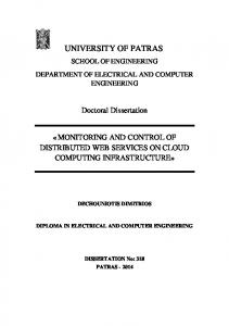
Generated using version 3.0 of the official AMS LATEX template

1

Computing and Partitioning Cloud Feedbacks using Cloud

2

Property Histograms.

3

Part II: Attribution to the Nature of Cloud Changes

Mark D. Zelinka

4

∗

Department of Atmospheric Sciences, University of Washington, Seattle, Washington,

and Program for Climate Model Diagnosis and Intercomparison, Lawrence Livermore National Laboratory, Livermore, California

Stephen A. Klein

5

Program for Climate Model Diagnosis and Intercomparison, Lawrence Livermore National Laboratory, Livermore, California

Dennis L. Hartmann

6

Department of Atmospheric Sciences, University of Washington, Seattle, Washington

Corresponding author address: Mark D. Zelinka, Program for Climate Model Diagnosis and Intercomparison Lawrence Livermore National Laboratory 7000 East Avenue, L-103 Livermore, CA 94551 E-mail: [email protected] ∗

1

7

ABSTRACT

8

Cloud radiative kernels and histograms of cloud fraction, both as functions of cloud

9

top pressure and optical depth, are used to quantify cloud amount, cloud height and cloud

10

optical depth feedbacks. The analysis is applied to doubled CO2 slab-ocean simulations

11

from ten global climate models participating in the Cloud Feedback Model Intercomparison

12

Project. In the ensemble mean, total cloud amount decreases, especially between 55◦ S

13

and 60◦ N, cloud altitude increases, and optical depths increase poleward of about 40◦ and

14

decrease at lower latitudes. Both longwave (LW) and shortwave (SW) cloud feedbacks are

15

positive, with the latter nearly twice as as large as the former. We show that increasing

16

cloud top altitude is the dominant contributor to the positive LW cloud feedback, and that

17

the extra-tropical contribution to the altitude feedback is approximately 70% as large as

18

the tropical contribution. In the ensemble mean, the positive impact of rising clouds is

19

50% larger than the negative impact of reductions in cloud amount on LW cloud feedback,

20

but the degree to which reductions in cloud fraction offset the effect of rising clouds varies

21

considerably across models. In contrast, reductions in cloud fraction make a large and

22

virtually unopposed positive contribution to SW cloud feedback, though the inter-model

23

spread is greater than for any other individual feedback component. In general, models

24

exhibiting greater reductions in subtropical marine boundary layer cloudiness tend to have

25

larger positive SW cloud feedbacks, in agreement with previous studies. Overall reductions

26

in cloud amount have twice as large an impact on SW fluxes as on LW fluxes such that

27

the net cloud amount feedback is moderately positive, with no models analyzed here having

28

a negative net cloud amount feedback. As a consequence of large but partially offsetting

29

effects of cloud amount reductions on LW and SW feedbacks, increasing cloud altitude 1

30

actually makes a greater contribution to the net cloud feedback than does the reduction in

31

cloud amount. Furthermore, the inter-model spread in net cloud altitude feedback is actually

32

larger than that of net cloud amount feedback. Finally, we find that although global mean

33

cloud optical depth feedbacks are generally smaller than the other components, they are

34

the dominant process at high latitudes. This large negative optical depth feedback at high

35

latitudes appears to result from a combination of increased cloud water content and changes

36

in phase from ice to liquid, not from increases in total cloud amount associated with the

37

poleward shift of the storm track, as is commonly assumed.

38

1. Introduction

39

Since the early days of climate modeling it has been recognized that changes in clouds

40

that accompany climate change provide a feedback through their large impact on the radia-

41

tion budget of the planet. As early as 1974, it was noted that accurate assessment of cloud

42

feedback requires quantifying the spatially-varying role of changes in cloud amount, height,

43

and optical properties on both shortwave (SW) and longwave (LW) radiation and that even

44

subtle changes to any of these properties can have significant effects on the planetary energy

45

budget (Schneider and Dickinson (1974)). Schneider (1972) performed one of the first inves-

46

tigations into the role of clouds as feedback mechanisms, focusing on hypothetical changes

47

in cloud amount and height. His calculations showed that a negative feedback would be

48

produced at most latitudes from an increase in low and middle-level clouds if albedo and

49

height were held fixed but that this effect could largely be cancelled by the enhanced cloud

50

greenhouse effect caused by a rise in global mean cloud top height of only a few tenths of 2

51

a kilometer, a result also supported by Cess (1974) and Cess (1975). Other early studies

52

focused on the potential increase in cloud optical depth that would occur in association with

53

global warming. Paltridge (1980), using the relationship between cloud optical depth and

54

liquid water path derived by Stephens (1978), showed that increases in liquid water path

55

would tend to strongly increase the amount of reflected SW radiation more than it would

56

decrease the amount of emitted LW radiation, resulting in a strong negative feedback on

57

a warming climate. These results were reinforced in the study of Somerville and Remer

58

(1984), who derived a large negative optical depth feedback using a 1-D radiative-convective

59

equilibrium model with empirically derived relations between temperature and cloud water

60

content measured by aircraft over the former Soviet Union (Feigelson (1978)). The adiabatic

61

increase of cloud liquid water path with temperature derived by Betts and Harshvardan

62

(1987) lent theoretical support to a cloud optical depth feedback.

63

Although 1-D radiative-convective equilibrium models employed to quantify cloud feed-

64

back in early studies like those described above provide insight into potential cloud feedbacks,

65

the cloud feedback operating in nature in response to external forcing is, as pointed out in

66

Schneider et al. (1978), made up of a complex mix of time, space, and radiation-weighted

67

cloud changes. The best chance to realistically simulate the response of clouds to external

68

forcing is with fully three-dimensional global climate models (GCMs). Some of the pioneer-

69

ing investigations into cloud feedback processes occurring in full three-dimensional GCMs

70

are those of Schneider et al. (1978) in the NCAR model, Manabe and Wetherald (1980)

71

and Wetherald and Manabe (1980) in the GFDL model, and Hansen et al. (1984) in the

72

GISS model. Inserting global mean cloud profiles produced by the GISS model for a control

73

and doubled-CO2 climate into the 1-D radiative convective equilibrium model of Lacis et al. 3

74

(1981), Hansen et al. (1984) calculated that cloud feedback represents a significant positive

75

feedback, made up of roughly equal contributions from decreased outgoing longwave radia-

76

tion due to increased cloud height and increased absorbed solar radiation due to decreased

77

cloud amount. Similar patterns of cloud changes, namely, a reduction in low and middle

78

level clouds and an increase in the height of tropical high clouds, were later found in the

79

GFDL model by Wetherald and Manabe (1988). Using the partial radiative perturbation

80

technique first introduced in Wetherald and Manabe (1980), they noted that the the LW

81

cloud amount and height feedbacks tended to oppose one another, resulting in a positive LW

82

cloud feedback that was roughly half as large as the positive SW cloud feedback.

83

Roeckner et al. (1987) performed the first doubled-CO2 GCM experiments in which cloud

84

liquid water was included prognostically, and found, after clarification by Schlesinger (1988),

85

that increases in cloud liquid water path and optical depth brought about a positive LW

86

optical depth feedback (due to increased high cloud emissivity) that dominated over the

87

smaller negative SW optical depth feedback (due to increased cloud reflectivity). This result

88

later received further support from the uniform ±2 K sea surface temperature perturbation

89

experiments of Taylor and Ghan (1992) for the NCAR model, but Senior and Mitchell (1993)

90

found that phase changes from ice to water in doubled CO2 experiments in the UK Met Office

91

model brought about large negative SW cloud feedbacks (which they defined as the change

92

in SW cloud radiative forcing), with contributions primarily coming from clouds at mid- and

93

high-latitudes.

94

Colman et al. (2001), using an earlier version of the BMRC model, performed perhaps

95

the most comprehensive analysis of cloud feedback due to a doubling of CO2 , separating

96

the feedback into components due to changes in cloud amount, height, and optical depth, 4

97

with the latter further broken down into components due to changes in total water, phase,

98

convective cloud fraction, and in-cloud temperature (a proxy for cloud geometric thickness).

99

Using the partial radiative perturbation method of Wetherald and Manabe (1980), they

100

computed large negative contributions to the LW cloud feedback from reductions in cloud

101

fraction and positive contributions from changes in cloud height and optical depth, the

102

latter dominated by increases in total water content of clouds. Conversely, they computed

103

large positive contributions to the SW cloud feedback from reductions in cloud amount and

104

increases in cloud height, but large negative contributions from increases in cloud optical

105

depth, the latter being primarily due to phase changes from ice to liquid, with a smaller

106

contribution from increases in total water content.

107

Though the issue of inter-model spread tends to dominate contemporary discussions of

108

cloud feedback, it is also important to identify, quantify, and understand which aspects are

109

robust and if there are fundamental physical explanations for such responses in a warming

110

climate. Common features to nearly all GCM studies of global warming due to increasing

111

greenhouse gas concentrations, including the early studies described above as well as the

112

current generation of climate models (c.f., Figure 10.10 of Meehl (2007)), are a decrease

113

in cloud amount equatorward of about 50◦ , an increase in cloud amount poleward of 50◦ ,

114

and an overall upward shift of clouds, features that mimic the average change in relative

115

humidity. Zelinka and Hartmann (2010) have argued that estimates of LW cloud feedback

116

in models taking part in CMIP3 are robustly positive and exhibit half as much inter-model

117

spread as those of SW cloud feedback because of the tendency for tropical high clouds to

118

rise in such a way as to remain at approximately the same temperature, a feature that Cess

119

(1974) and Cess (1975) advocated as appropriate for accurately describing the sensitivity 5

120

of clouds to surface temperature, and that is well-explained by the constraints of radiative-

121

convective equilibrium (Hartmann and Larson (2002)). Another feature that is emerging

122

as fairly robust across models is the large increase in cloud optical depth in the region of

123

mixed-phase clouds (roughly between 0◦ and -15◦ C) and smaller decrease at temperatures

124

greater than freezing (Mitchell et al. (1989); Senior and Mitchell (1993); Tselioudis et al.

125

(1998); Colman et al. (2001); Tsushima et al. (2006)).

126

In summary, models predict opposing effects on LW and SW radiation from changes

127

in cloud amount, altitude, and optical depth. The net cloud feedback thus represents the

128

integrated effect on radiation from spatially-varying – and in many cases subtle – cloud

129

amount, altitude, and optical depth responses that individually may have large magnitudes

130

and varying degrees of compensation. The relative magnitude of each of these processes

131

depends greatly on the details of each model’s cloud parameterization, such that even though

132

most models produce a similar gross change in cloud distribution, estimates of cloud feedback

133

remain widely spread relative to other feedbacks. Indeed, as first identified by Cess et al.

134

(1989) and Cess (1990), the variation in climate sensitivities predicted by GCMs is primarily

135

attributable to inter-model differences in cloud feedbacks. This continues to be the case in

136

contemporary climate models (Colman (2003); Soden and Held (2006); Ringer et al. (2006);

137

Webb et al. (2006)), and recent evidence has identified the response of marine boundary

138

layer clouds in subsidence regimes of the subtropics as primarily responsible for the inter-

139

model spread in cloud feedback (e.g., Bony et al. (2004); Bony and Dufresne (2005); Wyant

140

et al. (2006); Webb et al. (2006)). As we have noted in Part I, however, this should not be

141

taken as evidence that other cloud responses are consistently modelled or make a narrow

142

range of contributions to the feedback. The change in cloud properties and corresponding 6

143

cloud feedbacks are also likely to be strongly dependent on biases in their properties in the

144

unperturbed state, as pointed out by Trenberth and Fasullo (2010) for clouds in the high

145

latitudes of the Southern Hemisphere. Attribution of the mean and spread in cloud feedbacks

146

to the nature of the cloud changes from which they arise, which is the purpose of this paper,

147

is a necessary first step in identifying their robust and non-robust aspects and ultimately in

148

identifying which aspects are physically plausible and therefore realistic.

149

In Part I of this study (Zelinka et al. (2011a, manuscript submitted to J. Climate)

150

we proposed a new technique for computing cloud feedback using cloud radiative kernels

151

along with histograms of cloud fraction partitioned into CT P and τ bins by the Inter-

152

national Satellite Cloud Climatology Project (ISCCP) simulator (Klein and Jakob (1999);

153

Webb et al. (2001)). The technique has numerous appealing aspects, namely, the use of a

154

standard radiative transfer model and definition of cloudiness across models, the ability to

155

quantify the contribution to cloud feedback from individual cloud types, the exclusion of

156

any clear-sky changes that would otherwise require complicated corrections to infer a pure

157

cloud signal from changes in cloud radiative forcing, and the simplicity in the calculation

158

that requires neither high temporal resolution model output nor complicated substitution

159

techniques. Furthermore, cloud feedbacks computed with the cloud radiative kernels exhibit

160

close agreement with estimates of cloud feedback computed using the adjusted change in

161

cloud radiative forcing technique of Soden et al. (2008).

162

In this study, we extend further the capabilities of this technique to attribute cloud feed-

163

backs to the nature of cloud changes from which they arise in an ensemble of ten GCMs tak-

164

ing part in the first phase of the Cloud Feedback Model Intercomparison Project (CFMIP1).

165

Specifically, we use the cloud radiative kernels developed in Part I in combination with a 7

166

decomposition of the change in cloud fraction histograms to quantify the contribution from

167

amount, height, and optical depth changes to the ensemble mean and inter-model spread in

168

LW, SW, and net cloud feedbacks. Colman (2003), Soden and Held (2006), and Soden et al.

169

(2008) have provided intercomparisons of global mean cloud feedbacks in the current gener-

170

ation of GCMs, but none have separately quantified the cloud amount, altitude, and optical

171

depth feedbacks. Here we present the first model intercomparison of these components of

172

cloud feedback.

173

2. Partitioning Cloud Feedback by Decomposing the

174

Change in Cloud Distribution

175

We demonstrated in Part I that the cloud feedback estimated from the cloud radiative ker-

176

nel technique compares well with the feedback estimated independently by adjusting changes

177

in cloud radiative forcing for non-cloud effects using the technique outlined in Soden et al.

178

(2008). We also made use of the highly detailed information provided in the histograms to

179

partion the feedback into the various cloud types that cause it. However, the distinction be-

180

tween changes in cloud amount, height, and optical depth in contributing to cloud feedbacks

181

remained ambiguous. For example, high cloud changes dominate the LW cloud feedback

182

at all latitudes. This is unsurprising considering the high sensitivity of outgoing longwave

183

radiation (OLR) to high clouds as shown by the cloud radiative kernel, so even if the total

184

cloud fraction increased but the relative proportion of each cloud type in the histogram re-

185

mained unchanged, high clouds would stand out as being of primary importance. It is more

8

186

interesting and illuminating to quantify the contribution to the positive LW cloud feedback

187

of rising cloud tops relative to that of changes in total cloud amount holding the relative

188

proportions fixed. Similarly, it is desirable to separate the role of proportionate changes in

189

cloud fraction from that of a shift in the cloud optical depth distribution in contributing to

190

both LW and SW cloud feedbacks. The decomposition of cloud fraction changes proposed

191

here will remove some of the ambiguity associated with simply assessing cloud feedback from

192

changes in cloud fraction in specific bins of the histogram. In this section we present the methodology we use to decompose the change in cloud fraction into components due to the proportionate change in cloud fraction, the change in τ , and the change in CT P . The method is designed such that the feedback due to one of the three components (either cloud amount, altitude, or optical depth) is the result of only changes in that component with the other two components held fixed. To separate the effect of a change in mean cloud fraction from a shift in the altitude or optical depth of clouds, we divide the cloud fraction matrix into means over pressure and optical depth and departures therefrom. We note that several variants exist to define these feedbacks from ISCCP simulator output; we have chosen the most direct and simple method for our work, but we have seen little sensitivity to the method chosen. We will explain our methodology with the help of a 2x3 example matrix whose rows (columns) can be thought of as CT P (τ ) bins. The technique described below is applied in an analogous way to the full 7x7 matrix of the ISCCP simulator output. In our example, the CT P -τ matrix of the joint histogram

9

of cloud fraction for a single location and month for the current climate is given by, 



2 3 1 , C=   6 4 0 and an example matrix containing the change in cloud fraction, ∆C, between the current and 2xCO2 climate for this location and month is given by 



−1 0 2 . ∆C =    0 2 4 The hypothetical change in cloud fraction assuming the change in total cloud fraction is distributed throughout the histogram such that the relative proportions of cloud fractions in each CT P -τ bin remains constant is computed as:

∆Cprop = (

∆Ctot ) × C. Ctot

(1)

∆Ctot is the total change in cloud fraction computed as:

∆Ctot =

P X T X

∆C,

(2)

C,

(3)

p=1 τ =1

and Ctot is the total cloud fraction computed as:

Ctot =

P X T X p=1 τ =1

10

where P and T are the number of CT P and τ bins in the histogram (in this example, 2 and 3, respectively). The first term in Equation 1 is a scalar representing the fractional change in total cloud fraction. This decomposition isolates the contribution of changes in total cloud fraction from changes in the vertical and optical depth distribution of clouds. Using the example values, 

∆Cprop =







2 3 1 0.88 1.31 0.44 7 . = ×    16  2.63 1.75 0.00 6 4 0

193

The sum of the ∆Cprop histogram is exactly equal to the change in total cloud fraction, but

194

constructed in such a way that the relative proportion of clouds in each bin remains constant.

195

We will refer to ∆Cprop as the proportionate change in cloud fraction. To compute the cloud

196

feedback associated it, which we refer to as the cloud amount feedback, we multiply this

197

matrix by the corresponding entries of the cloud kernel for its location and month. To compute the cloud altitude feedback, we compute the hypothetical change in the distribution of cloud fractions assuming the total cloud fraction as well as the relative proportion of cloud fraction in each τ bin remains constant. This is computed by performing the following subtraction at each pressure bin:

∆C∆p

P 1 X = ∆C − ∆C P p=1

(4)

This computation takes the anomalous cloud fraction histogram and subtracts from each τ bin the mean anomaly across all CT P bins. This decomposition isolates the contribution of changes in the vertical distribution of clouds from the changes in total cloud fraction and 11

changes in the optical depth distribution of clouds. Using the example values, 











−1 0 2 −0.50 1.00 3.00 −0.50 −1.00 −1.00  = − ∆C∆p =        0.50 1.00 1.00 −0.50 1.00 3.00 0 2 4 198

The sum of the ∆C∆p histogram is exactly zero and the relative proportion of clouds in each

199

τ bin remains constant. Stated another way, C and C + ∆C∆p have the same total amount

200

of cloud and relative proportion of clouds in each τ bin. Multiplying ∆C∆p by the cloud

201

kernel for this location and month yields the cloud altitude feedback. In a similar manner, to compute the optical depth feedback, we compute the hypothetical change in the distribution of cloud fractions assuming the total cloud fraction as well as the relative proportion of clouds in each CT P bin remains constant. This is computed by performing the following subtraction at each optical depth bin:

∆C∆τ

T 1X = ∆C − ∆C T τ =1

(5)

This computation takes the anomalous cloud fraction histogram and subtracts from each CT P bin the mean anomaly across all τ bins. This decomposition isolates the contribution of changes in the optical depth distribution of clouds from the changes in total cloud fraction and changes in the vertical distribution of clouds. Using the example values, 











−1 0 2 0.33 0.33 0.33 −1.33 −0.33 1.67  = − ∆C∆τ =        −2.00 0.00 2.00 2.00 2.00 2.00 0 2 4 202

The sum of the histogram is exactly zero and the relative proportion of clouds in each CT P 12

203

bin remains constant. Stated another way, C and C + ∆C∆τ have the same total amount of

204

cloud and relative proportion of clouds in each CT P bin. Multiplying ∆C∆τ by the cloud

205

kernel yields the cloud optical depth feedback. The sum of the three decomposed matrices should roughly reproduce the true ∆C matrix. However, a small residual may remain in one or more bins (as in this example). Summing ∆Cprop , ∆C∆p , and ∆C∆τ gives 



−0.96 −0.02 1.10 .    1.13 2.75 3.00 Note, however, that the sum of this matrix is constrained to exactly equal the true change in cloud fraction (7 in this example). The residual is 











−1 0 2 −0.96 −0.02 1.10 −0.04 0.02 0.90 . = − ∆Cresidual =        −1.13 −0.75 1.00 1.13 2.75 3.00 0 2 4 206

Although the residual term sums to zero by design, it does contribute to the cloud feedback

207

calculation because it is multiplied with the cloud radiative kernel before being summed.

208

As shown below, this is generally a small contribution because the first-order components

209

of the feedback are accounted for by the effect of cloud amount, altitude, and optical depth

210

changes.

13

211

3. Ensemble Mean Change in Cloud Properties

212

As an aid in interpretting the contributions to cloud feedbacks from the three types of

213

cloud changes decomposed above, in Figure 1 we show the ensemble mean change in total

214

cloud fraction, CT P , and the natural logarithm of τ .

215

computed by differencing the cloud fraction-weighted mean of the midpoints of each CT P

216

or ln(τ ) bin between the control and doubled CO2 climate. For simplicity, we will refer

217

to these as changes in CT P and ln(τ ) rather than as changes in cloud fraction-weighted

218

pressure and cloud fraction-weighted ln(τ ).

The latter two quantities are

219

Cloud fraction decreases nearly everywhere between 55◦ S and 60◦ N and increases nearly

220

everywhere poleward of these latitudes (Figure 1a). An exception to this pattern is a large

221

region of increased cloud fraction in the central Equatorial Pacific which results from an

222

eastward shift in convection tracking anomalously high SSTs. Cloud fraction reductions are

223

prominent in the subtropics, especially over the continents. Large increases in cloud fraction

224

tend to occur where regions formerly covered with sea ice become open water in the warmed

225

climate. The general pattern of a decrease in cloud fraction equatorward of 50◦ is consistent

226

with many previous studies (e.g., Wetherald and Manabe (1988); Senior and Mitchell (1993);

227

Colman et al. (2001); Meehl (2007)).

228

Changes in CT P (Figure 1b) are negative nearly everywhere except in regions that

229

become dominated by low cloud types (e.g., in the Arctic and in the Central Pacific just

230

south of the Equator). Note that these values represent the change in cloud fraction-weighted

231

pressure; thus a location in which the cloud regime changes between the two climates will

232

exhibit large changes in this quantity (e.g., if the regime switches from being dominated by

14

233

low clouds to one dominated by high clouds). Therefore it is inappropriate to consider the

234

value at every location on the map as representing a purely vertical shift with no influence

235

from changing cloud types. However, that the global mean change in CT P is negative

236

implies that clouds systematically rise as the planet warms. In the Tropics, this is consistent

237

with theory (Hartmann and Larson (2002)) and results of cloud resolving model experiments

238

(Kuang and Hartmann (2007); Tompkins and Craig (1999)) and other ensembles of GCM

239

experiments (Zelinka and Hartmann (2010)). In the extratropics, rising clouds are also

240

consistent with a rising tropopause from a warmer troposphere and colder stratosphere due

241

to CO2 (Kushner et al. (2001); Santer et al. (2003); Lorenz and DeWeaver (2007)).

242

The map of changes in ln(τ ) exhibits a remarkable structure characterized by large in-

243

creases in ln(τ ) at latitudes poleward of about 40◦ and generally smaller decreases at low

244

latitudes (Figure 1c). Increases in ln(τ ) associated with global warming extend farther equa-

245

torward over the continents and exhibit a large seasonal cycle (not shown) apparently driven

246

by the larger seasonal variation in temperature relative to the oceans. As in the case of

247

changes in CT P , it is important to keep in mind that the change in ln(τ ) does not dis-

248

tinguish between changes in cloud type and changes in optical thickness of a given cloud

249

type. The optical depth changes produced in the models are qualitatively consistent with

250

observationally-derived relationships between temperature and optical depth. Tselioudis

251

et al. (1992) and Tselioudis and Rossow (1994) show using ISCCP data that cloud optical

252

thickness increases with temperature for cold low clouds but decreases with temperature for

253

warm low clouds. Additionally, Lin et al. (2003) show using data from the Surface Heat Bud-

254

get of the Arctic Ocean (SHEBA) experiment that Arctic cloud geometric thickness tends

255

to increase with surface temperature, resulting in clouds with larger optical thicknesses. 15

256

The high latitude cloud optical thickness response is likely related to changes in the

257

phase and/or total water contents of clouds that lead to increases in optical thickness as

258

temperature increases. As evidence, the fractional change in total, ice, and liquid water

259

path is shown in Figure 2. The latter quantity is computed from the difference in the former

260

two quantities.

261

unambiguously separate these changes in grid-box mean water path into their contributions

262

from changes in cloud amount or in-cloud water paths, much less directly relate these water

263

path changes to optical depth changes. Nevertheless, large increases in total water path

264

occur at high latitudes (Figure 2a), and are clearly dominated by the liquid phase (Figure

265

2c).

Due to limitations in the archive of CFMIP1 cloud output we cannot

266

Several lines of evidence suggest that this is a realistic response of high latitude cloud

267

properties, and that such changes should result in a clouds becoming more optically thick.

268

The total water contents of liquid and ice clouds tend to increase with temperature in

269

observations (Feigelson (1978); Somerville and Remer (1984); Mace et al. (2001)) at rates

270

that may in some circumstances be related to the increase in adiabatic water content with

271

temperature (Betts and Harshvardan (1987)). Betts and Harshvardan (1987) demonstrate

272

analytically that the rate of change in cloud liquid water content as a function of temperature

273

is twice as large at high latitudes compared with low latitudes. Additionally, a higher

274

freezing level associated with a warmer atmosphere promotes more liquid phase clouds which

275

– because of the Bergeron-Findeisen effect – tend to precipitate less efficiently and have

276

larger water contents than ice or mixed-phase clouds (Senior and Mitchell (1993); Tsushima

277

et al. (2006)). Finally, even if total water content were to remain constant, the smaller size

278

of liquid droplets relative to ice crystals tends to enhance cloud reflectivity and therefore 16

279

increase optical depth.

280

4. Ensemble Mean Cloud Feedback Contributions

281

In Figure 3 we show the decomposed contributions to the ensemble and annual mean LW

282

cloud feedback. In this and all of the following figures, the uiuc and mpi echam5 models are

283

excluded for the reasons discussed in Part I, and the ensemble mean refers to the remaining

284

ten models.

285

change in the vertical distribution of clouds (i.e., rising cloud tops) is the dominant contrib-

286

utor to the LW cloud feedback (Figure 3c). A noteworthy feature is that the contribution of

287

rising cloud tops to the LW cloud feedback is large not only within the Tropics but also in the

288

extratropics. The extratropical (latitude > 30◦ ) LW cloud altitude feedback is roughly 70%

289

of that in the Tropics (0.37 and 0.52 W m−2 K−1 , respectively). Considering the robust in-

290

creases in tropopause height in the extratropics with global warming (Kushner et al. (2001);

291

Santer et al. (2003); Lorenz and DeWeaver (2007)) and the fact that most extratropical high

292

cloud tops are near the tropopause, this may strengthen our confidence in the realism of

293

rising extra-tropical clouds and their positive contribution to the LW cloud feedback. As in

294

Zelinka and Hartmann (2010), we find that the ensemble mean contribution of rising tropical

295

clouds to the LW cloud feedback (0.52 W m−2 K−1 ) is twice as large as the global mean LW

296

cloud feedback (0.26 W m−2 K−1 ).

Consistent with the results presented in Zelinka and Hartmann (2010), the

297

Globally, the impact of proportionate changes in cloud fraction on the LW cloud feedback

298

is -0.30 W m−2 K−1 (Figure 3b), while the impact of increasing height of clouds is 0.45 W

299

m−2 K−1 , 50% greater in magnitude. Though rising clouds remain the primary cause of LW 17

300

cloud feedback, reductions in total cloud amount offset more than half of the altitude effect.

301

Positive LW cloud feedback that was primarily attributed to rising tropical cloud tops in

302

Zelinka and Hartmann (2010) is supported here, but it is clear that rising extra-tropical

303

clouds and reductions in cloud amount are also of primary importance in the global average.

304

We are aware of no fundamental reasons to expect the upward shift to dominate over cloud

305

fraction reductions in bringing about a positive LW cloud feedback, as observed here and in

306

Zelinka and Hartmann (2010).

307

Finally, the contribution of changes in cloud optical depth is smaller in the global mean

308

than that due to changes in cloud amount and height, but it is nonetheless positive nearly

309

everywhere (Figure 3d). Notably, optical depth increases are the primary positive contribu-

310

tion to LW cloud feedback poleward of about 60◦ in both hemispheres, strongly opposing

311

the locally negative altitude feedback over the polar oceans. In the global mean, the posi-

312

tive contribution to LW cloud feedback from optical depth increases is roughly equal to the

313

combined contribution to LW cloud feedback from clouds rising and decreasing in fractional

314

coverage.

315

In Figure 4 we show the decomposed contributions to the ensemble and annual mean

316

SW cloud feedback. The dominant contributor to the SW cloud feedback at most locations

317

and in the global mean is the change in cloud fraction holding the vertical and optical depth

318

distribution fixed (Figure 4b). With the exception of the equatorial Pacific, where increases

319

in cloud fraction occur in the ensemble mean, reductions in cloud fraction in most locations

320

between 50◦ S and 65◦ N contribute to a positive SW cloud feedback. This is consistent with

321

the results of Trenberth and Fasullo (2009), who showed reductions in low cloud fraction

322

(as defined by the standard cloud fraction diagnostic provided by the modeling centers) 18

323

throughout this region coincident with increases in absorbed solar radiation over the 21st

324

Century.

325

Unsurprisingly, the impact of changes in cloud vertical distribution on SW fluxes is

326

negligible everywhere (Figure 4c), though the global average value is slightly negative owing

327

to the slight increase in SW flux sensitivity to cloud fraction changes with decreasing cloud

328

top pressure (c.f., Figure 1b of Part I).

329

In the global mean, the SW optical depth feedback is considerably smaller than the

330

SW cloud amount feedback, but is regionally very important (Figure 4d). In the tropical

331

western Pacific, high clouds become thicker, thus causing a locally negative SW optical

332

depth feedback. Elsewhere equatorward of about 40◦ , this feedback component is positive

333

due to decreases in τ of low- and mid-level clouds. Consistent with this, Tselioudis et al.

334

(1992), Tselioudis and Rossow (1994), and Chang and Coakley (2007) have shown using

335

satellite observations that low- and midlatitude boundary layer clouds experience a decrease

336

in optical depth as temperature increases. The most dramatic and robust feature of the

337

optical depth feedback is the presence of large negative values at high latitudes in either

338

hemisphere, which dominate the other contributions to SW cloud feedback. As discussed

339

in the previous section, several lines of evidence suggest that cold clouds are particularly

340

susceptible to increases in temperature that act to increase their optical depth, providing

341

a possible physical basis for the modeled increases in τ (Figure 1c) and for the subsequent

342

strong negative optical depth feedback at high latitudes shown here.

343

Trenberth and Fasullo (2010) assert that biases in the mean state of GCMs are leading to

344

cloud feedbacks over the high southern latitudes that cannot be realized. Specifically, they

345

argue that unrealistically small cloud fractions over the Southern Ocean in the mean state 19

346

permit unrealistically large cloud fraction increases as the planet warms. Here, however, we

347

show that it is not the increase in cloud fraction but rather the shift towards brighter clouds

348

that primarily causes this large negative cloud feedback. If cloud optical depth rather than

349

cloud amount is biased low, then it is quite possible that models produce unrealistic increases

350

in cloud brightness as the planet warms. Conversely, if cloud optical depth is biased high,

351

as has been shown in many studies (e.g., Lin and Zhang (2004); Zhang (2005)) then the

352

negative SW optical depth feedback is in fact underestimated compared to a model with

353

more realistic mean state optical depths, as discussed in Bony et al. (2006). Regardless,

354

as discussed above, several plausible explanations exist for why clouds, especially those at

355

high latitudes, should become more optically thick as the planet warms. Thus we consider

356

the simulated increases in reflected SW radiation found in the 50◦ -60◦ S latitude band to be

357

plausible.

358

In Figure 5 we show the decomposed contributions to the ensemble and annual mean

359

net cloud feedback, which is quite strongly positive (0.71 W m−2 K−1 ).

360

0.41 W m−2 K−1 contribution of rising cloud tops (Figure 5c) exceeds the 0.36 W m−2 K−1

361

contribution of proportionate changes in the amount of clouds (Figure 5b) to net cloud

362

feedback. This is not a trivial result. One could argue that fundamental constraints exist on

363

cloud height and its changes, namely, the location of radiatively-driven clear-sky convergence

364

in the tropics (Hartmann and Larson (2002); Zelinka and Hartmann (2010)), and the height

365

of the tropopause in the extra-tropics (Kushner et al. (2001); Santer et al. (2003); Lorenz

366

and DeWeaver (2007)), making this contribution to cloud feedback robust and relatively

367

well-explained. The contribution of optical depth changes, though small in the global mean

368

(0.09 W m−2 K−1 ), is the primary cause of the large negative values of net cloud feedback 20

Surprisingly, the

369

over the Arctic and Southern Ocean (Figure 5d). The effect of proportionate changes in

370

cloud fraction as well as the effect of changes in the optical depth distribution of clouds on

371

the net cloud feedback is dominated by the SW contribution (i.e., the net map looks like

372

the SW map) whereas the effect of changes in the vertical distribution of clouds on the net

373

cloud feedback is entirely due to the LW contribution (i.e., the net map looks like the LW

374

map). Large positive contributions from both the reduction in total cloud fraction and the

375

upward shift of clouds produces the positive net cloud feedback between 50◦ S and 65◦ N. The

376

large negative contribution from the increase in cloud optical thickness produces the large

377

negative cloud feedback over the Arctic and Southern Ocean.

378

That the cloud optical depth feedback dominates over the cloud amount feedback at high

379

latitudes is a surprising result considering the large locally negative cloud feedback is often

380

attributed (e.g., Weaver (2003); Vavrus et al. (2009); Wu et al. (2010)) to cloud fraction

381

increases associated with the poleward-shifted storm track (Hall et al. (1994), Yin (2005)).

382

Indeed, appreciable cloud fraction changes do occur at high latitudes (Figure 1a), and these

383

do contribute to the negative SW cloud feedback, but this decomposition shows that the

384

signal is dominated by increases in cloud optical thickness in this region, likely caused by

385

the combination of large increases in total cloud water and phase changes (Figure 2). One

386

must keep in mind, however, that the optical depth feedback as we have defined it does not

387

distinguish a change in optical depth due to morphological changes in cloud type (e.g., from

388

thin boundary layer clouds to thicker frontal clouds) that may be associated with a storm

389

track shift from a change in optical depth due to a change in optical properties of the cloud

390

types that are already present (e.g., thin boundary layer clouds becoming thicker).

391

To more completely illuminate the cloud changes that result in a change in cloud feedback 21

392

from positive to negative as one moves poleward, we show the changes that occur in the

393

Southern Hemisphere where land does not obscure a clear zonal mean signal. In particular,

394

we show the mean cloud fraction histograms in the control and doubled CO2 climates, their

395

difference, and the induced feedbacks for the 30◦ -50◦S region in Figure 6 and for the 50◦ -70◦ S

396

region in Figure 7.

397

features of the stratocumulus, frontal, and cirrus regimes identified by Williams and Webb

398

(2009), though clouds in the 50◦ -70◦ S region tend to be thinner and lower than those in the

399

30◦ -50◦ S region. The total cloud fraction is roughly 20% larger at 50◦ -70◦S. The change in

400

cloud fraction histogram that occurs due to climate change is remarkably different between

401

these two regions (Figures 6c and 7c). At 30◦ -50◦S, the primary change is a reduction in

402

cloudiness at low levels and an increase in the altitude of high clouds. In contrast, at 50◦ -

403

70◦ S, the primary change is an increase in cloudiness at large optical depths at all heights

404

and decreases in the amount of low optical depth clouds, with an overall small increase in

405

total cloudiness. An exception to this general shift of the distribution towards thicker clouds

406

is in the lowest CT P bin (i.e., the highest clouds), where cloud fraction increases occur in

407

every τ bin but more so at smaller optical depths, perhaps a signature of the increasing

408

altitiude of high thin cirrus.

In both regions, the mean cloud fraction histogram primarily exhibits

409

In the 30◦ -50◦S region, increased cloudiness at the highest levels contributes to a small

410

LW cloud feedback, but the positive contribution to SW cloud feedback from the large

411

reductions in cloud amount in most bins dominates the cloud feedback. The impacts of high

412

cloud changes on LW and SW fluxes largely offset each other, with the resultant large positive

413

net cloud feedback being primarily caused by reduced SW reflection from the reduction in

414

cloud at low and mid-levels. In contrast, at 50◦ -70◦ S, the shift towards thicker clouds gives 22

415

rise to a strong positive LW cloud feedback and negative SW cloud feedback, the latter

416

having nearly the same magnitude as the positive SW cloud feedback at 30◦-50◦ S. The effect

417

of thickening high clouds on LW and SW fluxes largely offset each other and the net cloud

418

feedback is dominated by the large shift towards thicker clouds at the lowest levels (likely

419

stratocumulus clouds), making it moderately negative.

420

A striking feature that is apparent from comparing panels a and b of Figures 6 and 7 is

421

the subtle nature of the changes that occur to the cloud fraction histograms in going from

422

a control to a perturbed climate. Without computing a difference histogram (panel c) it

423

is difficult to visually discern a difference in the mean cloud fraction histograms between

424

the two climate states. The change in cloud distribution between the perturbed and control

425

climate, though sufficiently large to induce significant effects on radiation, does not suggest a

426

dramatic change in the types of clouds present in these regions. That such subtle changes in

427

cloud distribution can produce large radiative fluxes is rather humbling in that it underscores

428

an acute challenge of constraining cloud feedbacks.

429

The changes in cloud distribution that occur likely reflect some combination of changes

430

in the relative proportion of cloud types present in each region and changes in the properties

431

of the cloud types already present. Indeed, the results of Williams and Webb (2009) suggest

432

that a combination of both processes is important in a similar ensemble of CFMIP1 models.

433

Specifically, they find that the relative frequency of occurrence of thicker cloud types increases

434

at the expense of thinner cloud types in high latitude regions, and that all high latitude cloud

435

regimes except the thin cirrus regime experience a negative change in net cloud forcing.

436

The ensemble mean zonal mean cloud feedbacks and their partitioning among the three

437

components described above (and the residual term not discussed above) are shown in Figure 23

438

8. The competing effects of rising cloud tops and decreasing cloud coverage on the LW cloud

439

feedback is apparent at most latitudes, with the LW cloud altitude feedback dominating at

440

most latitudes, especially in the deep Tropics and midlatitudes. Proportionate cloud changes

441

are the dominant contributor to the SW cloud feedback at nearly every latitude, except at

442

high latitudes where the large increase in optical depth dominates. The relative dominance of

443

each contributor to the net cloud feedback varies as a function of latitude, but all components

444

are generally positive except at high latitudes where the optical depth feedback is strong and

445

negative.

446

In agreement with the physical mechanisms discussed above, Figure 7b of Colman et al.

447

(2001) shows that the dominant contribution to the negative SW optical depth feedback

448

at high latitudes in the BMRC model comes from cloud phase changes. They also note

449

that the SW and LW cloud amount feedbacks oppose each other at most latitudes, with the

450

global mean SW cloud amount feedback having a magnitude 2.2 times as large as that of

451

the LW cloud amount feedback (-0.14 and 0.31 W m−2 K−1 for LW and SW, respectively).

452

Remarkably, this is exactly the same ratio observed here for the ensemble mean cloud amount

453

feedbacks (-0.3 and 0.66 W m−2 K−1 for LW and SW, respectively), and is also close to the

454

ratio reported in Taylor and Ghan (1992).

455

5. Inter-Model Spread in Cloud Feedback Contributions

456

In Figure 9 we show bar plots of the global mean contributions of each component to

457

the LW, SW, and net cloud feedbacks in each model. LW cloud feedback estimates span a

458

range of 0.88 W m−2 K−1 (from -0.12 to 0.76 W m−2 K−1 ), though only the bmrc1 model has 24

459

a negative value. (Note that neither of the two tests for proper simulator implementation

460

discussed in Part I could be performed for the bmrc1 model.) In every model, proportionate

461

reductions in global mean cloud fraction act to reduce the LW cloud feedback, with values

462

spanning a range of 0.59 W m−2 K−1 (from -0.65 to -0.06 W m−2 K−1 ). Increases in cloud top

463

altitude contribute positively to the LW cloud feedback in all models, with values spanning a

464

range of 0.74 W m−2 K−1 (from 0.06 to 0.80 W m−2 K−1 ), a spread that warrants increased

465

attention. Increases in cloud optical depth contribute positively to the LW cloud feedback

466

in all models, with values spanning a range of 0.50 W m−2 K−1 (from 0.03 to 0.53 W m−2

467

K−1 ).

468

Even though LW feedback is positive in all but one model, it is clear that the relative

469

contribution of cloud fraction changes (negative feedback) and cloud vertical distribution

470

changes (positive feedback) varies significantly between models. The ratio of the magnitude

471

of the LW altitude feedback to the magnitude of the LW cloud amount feedback in individual

472

models varies between 0.2 and 10.5. The high end is populated by models like cccma agcm4 0

473

and ncar ccsm3 0 that have very little cloud amount decrease and a large cloud-top pressure

474

response whereas models like bmrc1 and ipsl cm4 have the opposite proportionality. Thus,

475

while the LW feedback may almost always be positive in models, the spread in this feedback

476

and the relative role of cloud top pressure and cloud fraction responses does vary in a

477

non-trivial way. Colman and McAvaney (1997) also found a widely varying amount of

478

compensation between these two quantities, with resultant LW cloud feedbacks of different

479

signs and magnitudes across four modified versions of the BMRC model. This demonstrates

480

that large uncertainties remain in the response of clouds relevant to the LW cloud feedback,

481

which, along with the result from Part I that the spread in high cloud-induced LW and SW 25

482

cloud feedback estimates exhibits more spread than that due to low clouds, suggests that the

483

community should not focus solely on the implications of disparate responses of low cloud

484

for cloud feedback.

485

SW cloud feedback estimates span a range of 1.16 W m−2 K−1 (from -0.13 to 1.03 W m−2

486

K−1 ), though only the gf dl mlm2 1 model has a negative value. In all models, reductions

487

in global mean cloud fraction act to increase the SW cloud feedback, with values spanning

488

a range of 1.32 W m−2 K−1 (from 0.14 to 1.18 W m−2 K−1 ). The range of estimates of

489

this feedback component is the largest of all components among both the SW and LW cloud

490

feedbacks. Increases in cloud top altitude contribute negatively to the SW cloud feedback

491

in all models, but the values are very small, in no models exceeding -0.08 W m−2 K−1 . SW

492

optical depth feedback estimates span a range of 0.80 W m−2 K−1 (from -0.58 to 0.22 W

493

m−2 K−1 ).

494

Net cloud feedback estimates are positive in all models, spanning a range of 0.92 W m−2

495

K−1 (from 0.22 to 1.14 W m−2 K−1 ). Proportionate reductions in global mean cloud fraction

496

act to give a positive net cloud feedback, with values spanning a range of 0.63 W m−2 K−1

497

(from 0.07 to 0.70 W m−2 K−1 ). In every model, increases in cloud top altitude contribute

498

positively to the net cloud feedback, with values spanning a range of 0.66 W m−2 K−1 (from

499

0.06 to 0.72 W m−2 K−1 ). The strength of this component of the feedback has a larger inter-

500

model spread than that of the cloud amount component, which is surprising considering the

501

large focus placed on the implications of the disparate responses of subtropical boundary

502

layer cloud amounts. Net optical depth feedback estimates span a range of 0.44 W m−2 K−1

503

(from -0.10 to 0.34 W m−2 K−1 ). Only two models (bmrc1 and gf dl mlm2 1) have negative

504

net optical depth feedbacks. 26

505

To display these results in a more compact manner, in Figure 10 we show global mean

506

cloud feedback estimates and their partitioning among cloud amount, altitude, optical depth

507

and residual components.

508

itive LW cloud feedback is the upward shift of clouds, with a smaller positive contribution

509

from cloud thickening and a moderate negative contribution from cloud fraction decreases.

510

Decreasing cloud amount makes by far the largest contribution to SW cloud feedback. Note

511

that while the SW optical depth feedback makes little contribution to the global mean SW

512

cloud feedback, it is the dominant feedback at high latitudes. Both the cloud altitude feed-

513

back and the cloud amount feedback contribute to the strong positive net cloud feedback. In

514

the global mean, optical depth changes make a smaller positive contribution that is opposed

515

by the negative effect of residual cloud changes.

As mentioned previously, the dominant contributor to the pos-

516

Considerable inter-model spread is evident in most contributions to cloud feedback, with

517

the SW cloud amount feedback exhibiting the largest spread. Due to the small sample

518

size of only 10 models, regression coefficients of global mean cloud feedback components on

519

global mean cloud feedback are indistinguishable from zero in most cases (regression slope

520

uncertainty taken to be the 2σ range of the distribution of regression slopes computed using a

521

bootstrapping method in which the predictand is resampled 1000 times). This demonstrates

522

that inter-model spread is liberally distributed between component changes and LW and

523

SW bands with no single component playing a dominant role. Two exceptions are the

524

large positive regression coefficient between global mean SW cloud feedback and its amount

525

component (0.77±0.47) and large positive regression coefficient between global mean LW

526

cloud feedback and its altitude component (0.62±0.37). This leads to the result that models

527

having greater positive SW cloud amount feedbacks (i.e., those with larger reductions in cloud 27

528

fraction) tend to have greater global mean SW cloud feedbacks and models having greater

529

positive LW cloud altitude feedbacks tend to have greater positive LW cloud feedbacks. The

530

spread in the LW cloud altitude feedback may be related to the inter-model spread in the

531

vertical shift of peak radiatively-driven divergence in the Tropics and the tropopause height

532

in the extratropics, which suggests that the spread in this feedback process can be explained

533

simply by the spread in responses of models’ vertical temperature structures. We do not

534

attempt to demonstrate this here, as few models archived atmospheric temperature profiles;

535

thus it remains speculation.

536

A regression of the global mean feedbacks on their values from each grid point can also be

537

performed, highlighting the local contribution of each process to the spread in global mean

538

cloud feedbacks, but at most locations, the regression slopes are statistically indistinguishable

539

from zero. Regions that tend to be dominated by stratiform clouds over the subtropical

540

oceans off the west coast of continents are among the regions (though not the only regions)

541

for which the regression slope is significantly positive, indicating that an appreciable portion

542

of the spread in global mean SW cloud feedback is attributable to the inter-model spread

543

in the response of these clouds types. Models in which the SW cloud amount feedback is

544

positive in these regions (i.e., models in which the amount of these clouds decreases) tend to

545

be models having larger positive global mean SW cloud feedbacks, a result consistent with

546

several others (Bony et al. (2004); Bony and Dufresne (2005); Wyant et al. (2006); Webb

547

et al. (2006)).

28

548

6. Conclusions

549

We have proposed a decomposition of the change in cloud fraction histogram which

550

separates cloud changes into components due to the proportionate change in cloud fraction

551

holding the vertical and optical depth distribution fixed, the change in vertical distribution

552

holding the optical depth distribution and total cloud amount fixed, and the change in

553

optical depth distribution holding the vertical distribution and total cloud amount fixed. By

554

multiplying the cloud radiative kernels developed in Part I with these decomposed changes

555

in cloud fraction (normalized by the change in global mean surface temperature), we have

556

computed the cloud amount, altitude, and optical depth feedbacks for an ensemble of ten

557

models taking part in CFMIP1, allowing us to assess for the first time the relative roles of

558

these processes in determining both the multi-model mean and inter-model spread in LW,

559

SW, and net cloud feedback.

560

In agreement with many previous studies, a warmed climate is associated with a reduction

561

in total cloud amount between about 55◦ S and 60◦ N, an increase in cloud amount poleward

562

of these latitudes, an upward shift of clouds at nearly every location, an increase in cloud

563

optical depth poleward of about 40◦ , and a generally much smaller decrease in cloud optical

564

depth equatorward of 40◦ . We note that both changes in total water path and in phase from

565

ice to liquid contributes to a shift towards brighter clouds at high latitudes, a feature that is

566

in agreement with many studies (e.g., Somerville and Remer (1984); Betts and Harshvardan

567

(1987); Tsushima et al. (2006)). However, we have noted that – even in regions where

568

cloud changes are substantial enough to make large contributions to cloud feedback – a

569

visual comparison of cloud fraction histograms in the control and perturbed climate reveals

29

570

a nearly indiscernible change in cloud properties. This highlights the concept that large

571

changes in radiation can arise from very subtle cloud changes. A related point not explored

572

here is that multi-decadal averages are necessary to discern these changes, which, while

573

small, are still very important for cloud feedback.

574

Before summarizing our cloud feedback results, we wish to stress that our results are

575

applicable specifically to this ensemble of ten global climate models coupled to slab oceans

576

in which CO2 is instantaneously doubled and the climate is allowed to re-equilibrate. Thus

577

one should not expect perfect overlap between the estimates of cloud feedback shown here

578

and those presented, for example, in Soden et al. (2008), who analyzed transient climate

579

feedbacks computed as a difference between years 2000-2010 and 2090-2100 in an ensemble

580

of 14 fully coupled ocean-atmosphere GCMs simulating the SRES A1B scenario, in which the

581

concentrations of numerous radiative agents vary over the course of the century (Ramaswamy

582

et al. (2001)), as well as among models (e.g., Collins (2006); Shindell et al. (2008)). Indeed,

583

here we found a moderately large positive ensemble mean SW cloud feedback of 0.46 W

584

m−2 K−1 and a LW cloud feedback that is roughly half as large, 0.26 W m−2 K−1 , whereas

585

these values in GCMs simulating the SRES A2 scenario are 0.09 and 0.49 W m−2 K−1 ,

586

respectively (c.f., Figure 2 of Zelinka and Hartmann 2011a, manuscript submitted to J.

587

Climate). While the exact values of global mean feedbacks may differ somewhat between

588

the type of model run, we still expect that the important processes identified in this study

589

to be relevant for other types of simulations such as transient climate change integrations of

590

coupled ocean-atmosphere GCMs driven by gradual increases in greenhouse gases.

591

Rising clouds contribute positively to the LW cloud feedback in every model, and rep-

592

resent the dominant contributor to the positive ensemble mean LW cloud feedback, lending 30

593

further support to the conclusions of Zelinka and Hartmann (2010). Although that study fo-

594

cused solely on the contribution of rising tropical clouds to the positive LW cloud feedback,

595

here we see that rising extratropical clouds also contribute significantly, with a contribu-

596

tion that is roughly 70% as large as that from tropical clouds. As a deeper troposphere

597

is a consistently-modeled and theoretically-expected feature of a warming climate due to

598

increased CO2 , the rise of clouds and its attendant large positive contribution to LW cloud

599

feedback may be considered robust and well-explained. The impact of reductions in cloud

600

amount on LW cloud feedback, however, systematically opposes that of increases in cloud

601

altitude, and the ratio of the two components varies considerably between models, indicating

602

that substantial inter-model variability exists in the response of high clouds, with implica-

603

tions for the size of LW cloud feedback. Nevertheless, in the ensemble mean, the LW cloud

604

altitude feedback is roughly 50% larger than the LW cloud amount feedback. Interestingly,

605

optical depth increases make a small positive contribution to the LW cloud feedback in ev-

606

ery model, which, in the ensemble mean, is equal to the combined LW altitude plus amount

607

feedback.

608

Overall reductions in cloud amount are by far the dominant contributor to the positive

609

SW cloud feedback, and represent the largest individual contribution to the positive global

610

mean cloud feedback in this ensemble of models. Although this component is positive in

611

every model due to the robust reduction in global mean cloudiness, it exhibits the largest

612

inter-model spread of all feedback components. The positive contribution from cloud amount

613

reductions to SW cloud feedback is a little more than twice as large as the magnitude of its

614

negative contribution to LW cloud feedback, highlighting the importance of reductions in low

615

and middle level clouds. This factor of two is in remarkable agreement with results from both 31

616

the NCAR model experiment of Taylor and Ghan (1992) and the BMRC model experiment

617

of Colman et al. (2001). Models with larger reductions in cloud amount in regions typically

618

occupied by marine stratocumulus tend to have larger positive SW cloud feedbacks, a result

619

in agreement with many previous studies (e.g., Bony et al. (2004); Bony and Dufresne (2005);

620

Webb et al. (2006); Wyant et al. (2006)). The SW optical depth feedback is small globally,

621

but is the dominant feedback at high latitudes, where the combination of increased cloud

622

water content and phase change from ice to liquid increases the mean cloud optical depth.

623

That the SW optical depth feedback dominates over the SW cloud amount feedback at high

624

latitudes suggests that increases in net moisture transport and the liquid water content of

625

clouds are more important than the poleward shift of the extratropical storm tracks that

626

occurs in warming simulations.

627

The net cloud feedback represents the integrated effect of large, spatially heterogeneous,

628

and in many cases opposing effects on the radiation budget. Nevertheless, it is positive in

629

every model, as are the contributions from decreasing cloud amount and increasing cloud

630

altitude. Interestingly, increasing cloud altitude makes a larger contribution to net cloud

631

feedback than does decreasing cloud amount, and does so in seven out of ten models. This

632

is because LW and SW cloud amount feedbacks tend to offset each other, while the positive

633

impact of cloud height changes on the LW cloud feedback is largely unopposed. Although

634

only two models have negative global mean optical depth feedbacks, all models exhibit large

635

negative optical depth feedbacks at high latitudes. This locally large negative feedback is due

636

primarily to low clouds becoming thicker, since the increased optical depth of high clouds

637

has compensating effects on LW and SW radiation.

32

638

Acknowledgments.

639

This research was supported by the Regional and Global Climate Program of the Of-

640

fice of Science at the U. S. Department of Energy and by NASA Grant NNX09AH73G

641

at the University of Washington. We acknowledge the international modeling groups, the

642

Program for Climate Model Diagnosis and Intercomparison (PCMDI), and the WCRP’s

643

Working Group on Coupled Modelling (WGCM) for their roles in making available the

644

WCRP CFMIP multi-model dataset. Support of this dataset is provided by the Office of

645

Science, U.S. Department of Energy. We thank Brian Soden for providing the radiative

646

kernels, Rick Hemler for providing additional gf dl mlm2 1 model output, Rob Wood, Chris

647

Bretherton, and Robert Pincus for useful discussion and suggestions for improvement, and

648

Marc Michelsen for computer support. This work was performed under the auspices of the

649

U.S. Department of Energy by Lawrence Livermore National Laboratory under Contract

650

DE-AC52-07NA27344.

33

651

652

REFERENCES

653

Betts, A. K. and Harshvardan, 1987: Thermodynamic constraint on the cloud liquid water

654

feedback in climate models. J. Geophys. Res., 92, 8483–8485.

655

Bony, S. and J. L. Dufresne, 2005: Marine boundary layer clouds at the heart of tropical

656

cloud feedback uncertainties in climate models. Geophys. Res. Lett., 32, L20806, doi:

657

10.1029/2005GL023851.

658

659

660

661

Bony, S., J. L. Dufresne, H. L. Treut, J. J. Morcrette, and C. Senior, 2004: On dynamic and thermodynamic components of cloud changes. Climate Dyn., 22, 71–68. Bony, S., et al., 2006: How well do we understand and evaluate climate change feedback processes? J. Climate, 19, 3445–3482.

662

Cess, R. D., 1974: Radiative transfer due to atmospheric water vapor: Global considerations

663

of Earth’s energy balance. Journal of Quantitative Spectroscopy and Radiative Transfer,

664

14 (9), 861–871.

665

666

667

668

Cess, R. D., 1975: Global climate change - investigation of atmospheric feedback mechanisms. Tellus, 27 (3), 193–198. Cess, R. D., et al., 1989: Interpretation of cloud-climate feedback as produced by 14 atmospheric general circulation models. Science, 245 (4917), 513–516.

34

669

Cess, R. D. e. a., 1990: Intercomparison and interpretation of cloud-climate feedback pro-

670

cesses in nineteen atmospheric general circulation models. J. Geophys. Res., 95, 16 601–

671

16 615.

672

Chang, F.-L. and J. A. Coakley, 2007: Relationships between marine stratus cloud optical

673

depth and temperature: Inferences from AVHRR observations. J. Climate, 20 (10), 2022–

674

2036.

675

Collins, W. D. e. a., 2006: Radiative forcing by well-mixed greenhouse gases: Estimates

676

from climate models in the Intergovernmental Panel on Climate Change (IPCC) Fourth

677

Assessment Report (AR4). J. Geophys. Res., 111, D14317, doi:10.1029/2005JD006713.

678

Colman, R., 2003: A comparison of climate feedbacks in general circulation models. Climate

679

680

681

Dyn., 20, 865–873. Colman, R., J. Fraser, and L. Rotstayn, 2001: Climate feedbacks in a general circulation model incorporating prognostic clouds. Climate Dyn., 18, 103–122.

682

Colman, R. and B. McAvaney, 1997: A study of general circulation model climate feedbacks

683

determined from perturbed sea surface temperature experiments. J. Geophys. Res., 102,

684

19 383–19 402.

685

686

Feigelson, E. M., 1978: Preliminary radiation model of a cloudy atmosphere. Part I: Structure of clouds and solar radiation. Beitr. Phys. Atmos., 51, 203–229.

687

Hall, N. M. J., B. J. Hoskins, P. J. Valdes, and C. A. Senior, 1994: Storm tracks in a high-

688

resolution gcm with doubled carbon dioxide. Quart J Roy Meteorol Soc, 120, 1209–1230.

35

689

Hansen, J., A. Lacis, D. Rind, G. Russell, P. Stone, I. Fung, R. Ruedy, and J. Lerner, 1984:

690

Climate processes and climate sensitivity: Analysis of feedback mechanisms. Geophys.

691

Monogr., 29, 130–163.

692

693

694

695

696

697

698

699

700

701

Hartmann, D. L. and K. Larson, 2002: An important constraint on tropical cloud-climate feedback. Geophys. Res. Lett., 29 (20), doi:10.1029/2002GL015835. Klein, S. A. and C. Jakob, 1999: Validation and sensitivities of frontal clouds simulated by the ECMWF model. Mon. Weath. Rev., 127, 2514–2531. Kuang, Z. and D. L. Hartmann, 2007: Testing the fixed anvil temperature hypothesis in a cloud-resolving model. J. Climate, 20, 2051–2057. Kushner, P. J., I. M. Held, and T. L. Delworth, 2001: Southern hemisphere atmospheric circulation response to global warming. J. Climate, 14 (10), 2238–2249. Lacis, A., J. Hansen, P. Lee, T. Mitchell, , and S. Lebedeff, 1981: Greenhouse effect of trace gases, 1970-1980. Geophys. Res. Lett., 8 (10), 1035–1038.

702

Lin, B., P. Minnis, and A. Fan, 2003: Cloud liquid water path variations with temperature

703

observed during the Surface Heat Budget of the Arctic Ocean (SHEBA) experiment. J.

704

Geophys. Res., 108, doi:10.1029/2002JD002851.

705

Lin, W. Y. and M. H. Zhang, 2004: Evaluation of clouds and their radiative effects simulated

706

by the NCAR Community Atmospheric Model against satellite observations. J. Climate,

707

17 (17), 3302–3318.

708

Lorenz, D. J. and E. T. DeWeaver, 2007: Tropopause height and zonal wind response to 36

709

global warming in the IPCC scenario integrations. J. Geophys. Res., 112, D10119, doi:

710

10.1029/2006JD008087.

711

Mace, G. G., E. E. Clothiaux, and T. P. Ackerman, 2001: The composite characteristics

712

of cirrus clouds: Bulk properties revealed by one year of continuous cloud radar data. J.

713

Climate, 14, 2185–2203.

714

715

716

717

718

719

720

721

722

723

724

725

726

727

Manabe, S. and R. T. Wetherald, 1980: On the distribution of climate change resulting from an increase in CO2 content of the atmosphere. J. Atmos. Sci., 37 (1), 99–118. Meehl, G. A. e. a., 2007: Global climate projections. Climate Change 2007: The Physical Science Basis, S. S. et al., Ed., Cambridge University Press, 747–846. Mitchell, J. F. B., C. A. Senior, and W. J. Ingram, 1989: C02 and climate: a missing feedback? Nature, 341, 132–134. Paltridge, G. W., 1980: Cloud-radiation feedback to climate. Quart. J. Roy. Meteor. Soc., 106 (450), 895–899. Ramaswamy, V. et al., 2001: Radiative forcing of climate change. Climate Change 2001: The Scientific Basis, J. T. H. et al., Ed., Cambridge University Press, 350–416. Ringer, M. A., et al., 2006: Global mean cloud feedbacks in idealized climate change experiments. Geophys. Res. Lett., 33, L07718, doi:10.1029/2005GL025370. Roeckner, E., U. Schlese, J. Biercamp, and P. Liewe, 1987: Cloud optical depth feedback and climate modeling. Nature, 329, 138–139.

37

728

729

730

731

Santer, B. D., et al., 2003: Contributions of anthropogenic and natural forcing to recent tropopause height changes. Science, 301 (5632), 479–483. Schlesinger, M. E., 1988: Negative or positive cloud optical depth feedback? Nature, 335, 303–304.

732

Schneider, S. H., 1972: Cloudiness as a global climatic feedback mechanism: The effects

733

on radiation balance and surface-temperature of variations in cloudiness. J. Atmos. Sci.,

734

29 (8), 1413–1422.

735

736

Schneider, S. H. and R. E. Dickinson, 1974: Climate modeling. Reviews of Geophysics, 12 (3), 447–493.

737

Schneider, S. H., W. M. Washington, and R. M. Chervin, 1978: Cloudiness as a climatic

738

feedback mechanism: Effects on cloud amounts of prescribed global and regional surface

739

temperature changes in the NCAR GCM. J. Atmos. Sci., 35 (12), 2207–2221.

740

741

Senior, C. and J. Mitchell, 1993: Carbon dioxide and climate. The impact of cloud parameterization. J. Climate, 6, 393–418.

742

Shindell, D. T., H. Levy, M. D. Schwarzkopf, L. W. Horowitz, J.-F. Lamarque, and G. Falu-

743

vegi, 2008: Multimodel projections of climate change from short-lived emissions due to

744

human activities. J. Geophys. Res., 113, D11109, doi:10.1029/2007JD009152.

745

746

Soden, B. J. and I. M. Held, 2006: An assessment of climate feedbacks in coupled oceanatmosphere models. J. Climate, 19, 3354–3360.

38

747

748

749

750

751

752

753

754

755

756

757

758

759

760

Soden, B. J., I. M. Held, R. Colman, K. M. Shell, J. T. Kiehl, and C. A. Shields, 2008: Quantifying climate feedbacks using radiative kernels. J. Climate, 21, 3504–3520. Somerville, R. C. J. and L. A. Remer, 1984: Cloud optical thickness feedbacks in the CO2 climate problem. J. Geophys. Res., 89 (D6), 9668–9672. Stephens, G. L., 1978: Radiation profiles in extended water clouds. Part II: Parameterization schemes. J. Atmos. Sci., 35 (11), 2123–2132. Taylor, K. E. and S. J. Ghan, 1992: An analysis of cloud liquid water feedback and global climate sensitivity in a general circulation model. J. Climate, 5 (9), 907–919. Tompkins, A. M. and G. C. Craig, 1999: Sensitivity of tropical convection to sea surface temperature in the absence of large-scale flow. J. Climate, 12, 462–476. Trenberth, K. E. and J. T. Fasullo, 2009: Global warming due to increasing absorbed solar radiation. Geophys. Res. Lett., 36, L07706, doi:10.1029/2009GL037527. Trenberth, K. E. and J. T. Fasullo, 2010: Simulation of present-day and twenty-first-century energy budgets of the southern oceans. J. Climate, 23 (2), 440–454.

761

Tselioudis, G., A. D. D. Genio, W. Kovari, and M.-S. Yao, 1998: Temperature dependence

762

of low cloud optical thickness in the GISS GCM: Contributing mechanisms and climate

763

implications. J. Climate, 11 (12), 3268–3281.

764

765

Tselioudis, G. and W. B. Rossow, 1994: Global, multiyear variations of optical thickness with temperature in low and cirrus clouds. Geophys. Res. Lett., 21(20), 2211–2214.

39

766

767

Tselioudis, G., W. B. Rossow, and D. Rind, 1992: Global patterns of cloud optical thickness variation with temperature. J. Climate, 5, 1484–1495.

768

Tsushima, Y., et al., 2006: Importance of the mixed-phase cloud distribution in the control

769

climate for assessing the response of clouds to carbon dioxide increase: A multi-model

770

study. Climate Dyn., 27, 113–126.

771

Vavrus, S., D. Waliser, A. Schweiger, and J. Francis, 2009: Simulations of 20th and 21st

772

century Arctic cloud amount in the global climate models assessed in the IPCC AR4.

773

Climate Dyn., 33, 1099–1115.

774

Weaver, C. P., 2003: Efficiency of storm tracks an important climate parameter? The

775

role of cloud radiative forcing in poleward heat transport. J. Geophys. Res., 108, doi:

776

10.1029/2002JD002756.

777

Webb, M., C. Senior, S. Bony, and J. J. Morcrette, 2001: Combining ERBE and ISCCP data

778

to assess clouds in the Hadley Centre, ECMWF and LMD atmospheric climate models.

779

Climate Dyn., 17, 905–922.

780

781

782

783

784

785

Webb, M. J., et al., 2006: On the contribution of local feedback mechanisms to the range of climate sensitivity in two gcm ensembles. Climate Dyn., 27, 17–38. Wetherald, R. and S. Manabe, 1988: Cloud feedback processes in a general circulation model. J. Atmos. Sci., 45, 1397–1415. Wetherald, R. T. and S. Manabe, 1980: Cloud cover and climate sensitivity. J. Atmos. Sci., 37 (7), 1485–1510.

40

786

787

Williams, K. and M. Webb, 2009: A quantitative performance assessment of cloud regimes in climate models. Climate Dyn., 33, 141–157.

788

Wu, Y., M. Ting, R. Seager, H.-P. Huang, and M. Cane, 2010: Changes in storm tracks and

789

energy transports in a warmer climate simulated by the GFDL CM2.1 model. Climate

790

Dyn., 1–20, doi:10.1007/s00382-010-0776-4.

791

Wyant, M. C., C. S. Bretherton, J. T. Bacmeister, J. T. Kiehl, I. M. Held, M. Zhao, S. A.

792

Klein, and B. J. Soden, 2006: A comparison of low-latitude cloud properties and responses

793

in agcms sorted into regimes using mid-tropospheric vertical velocity. Climate Dyn., 27,

794

261–279.

795

796

797

798

Yin, J. H., 2005: A consistent poleward shift of the storm tracks in simulations of 21st century climate. Geophys. Res. Lett., 32, L18701, doi:10.1029/2005GL023684. Zelinka, M. D. and D. L. Hartmann, 2010: Why is longwave cloud feedback positive? J. Geophys. Res., 115, D16117, doi:10.1029/2010JD013817.

799

Zhang, M. H. e. a., 2005: Comparing clouds and their seasonal variations in 10 atmospheric

800

general circulation models with satellite measurements. J. Geophys. Res., 110, D15S02,

801

doi:10.1029/2004JD005021.

41

802

803

List of Figures 1

Ensemble mean change in (a) cloud fraction, (b) cloud fraction-weighted pres-

804

sure, and (c) cloud fraction-weighted natural logarithm of optical depth. The

805

ensemble mean refers to all models except the uiuc and mpi echam5 models,

806

which are excluded based on discrepancies discussed in the companion paper.

807

2

44

Ensemble mean change in (a) total water path, (b) ice water path, and (c)

808

liquid water path. The ensemble mean refers to all models except the uiuc

809

and mpi echam5 models. The bmrc1, ipsl cm4, and miroc hisens models are

810

also excluded because they did not archive total water path or ice water path. 45

811

3

Ensemble and annual mean (a) LW cloud feedback and components due to the

812

(b) proportionate change in cloud fraction, (c) change in cloud vertical distri-

813

bution, (d) change in cloud optical depth distribution, and (e) residual term.

814

The ensemble mean refers to all models except the uiuc and mpi echam5

815

models.

46

816

4

As in Figure 3, but for the SW cloud feedback partitioning.

47

817

5

As in Figure 3, but for the net cloud feedback partitioning.

48

818

6

Mean cloud fraction in the 30◦ -50◦S region for the (a) 1xCO2 and (b) 2xCO2

819

runs of all models except uiuc and mpi echam5, along with (c) the difference

820

expressed per unit change in each model’s global mean surface temperature

821

between the two states. Multiplication of the histogram of the change in

822

cloud fraction with the (d) LW, (e) SW, and (f) net cloud radiative kernel

823

histogram. The sum of each histogram is shown in each title.

42

49

824

7

As in Figure 6, but for the 50◦ -70◦S region.

825

8

Zonal mean ensemble mean (a) LW, (b) SW, and (c) net cloud feedbacks par-

826

titioned into components due to the proportionate change in cloud fraction,

827

change in cloud vertical distribution, change in cloud optical depth distribu-

828

tion, and residual term. The abscissa is sine of latitude so that the visual inte-

829

gral is proportional to Watts per Kelvin of mean surface temperature change.

830

The ensemble mean refers to all models except the uiuc and mpi echam5

831

models.

832

9

51

Global mean cloud feedbacks estimated for each model using (green) the ad-

833

justed change in cloud radiative forcing technique of Soden et al. (2008) and

834

(black) cloud radiative kernels. Also shown is the contribution to the feedback

835

of (blue) amount, (cyan) altitude, (red) optical depth, and (maroon) residual

836

changes.

837

10

50

52

Global mean (red) LW, (blue) SW, and (black) net cloud feedback estimates

838

and the contribution to the cloud feedbacks from the proportionate change in

839

cloud fraction, change in cloud vertical distribution, change in cloud optical

840

depth distribution, and residual term. Each model is represented by a dot

841

and the multi-model mean is represented by the height of the vertical bar.

842

The uiuc and mpi echam5 models are excluded from this figure.

43

53

(a) ∆Ctot 3 2 1 0 −1 −2 −3 −1

Global Mean = −0.4 % K (b) ∆CTP

20 15 10 5 0 −5 −10 −15 −20 −1

Global Mean = −4.05 hPa K (c) ∆ln(τ)

0.3 0.2 0.1 0 −0.1 −0.2 −0.3 −1

Global Mean = 0.03 K

Fig. 1. Ensemble mean change in (a) cloud fraction, (b) cloud fraction-weighted pressure, and (c) cloud fraction-weighted natural logarithm of optical depth. The ensemble mean refers to all models except the uiuc and mpi echam5 models, which are excluded based on discrepancies discussed in the companion paper.

44

(a) ∆ Total Water Path 30 20 10 0 −10 −20 −30

Global Mean = 1.88 % K−1 (b) ∆ Ice Water Path 30 20 10 0 −10 −20 −30 −1

Global Mean = 0.03 % K (c) ∆ Liquid Water Path

30 20 10 0 −10 −20 −30 −1

Global Mean = 4.2 % K

Fig. 2. Ensemble mean change in (a) total water path, (b) ice water path, and (c) liquid water path. The ensemble mean refers to all models except the uiuc and mpi echam5 models. The bmrc1, ipsl cm4, and miroc hisens models are also excluded because they did not archive total water path or ice water path.

45

Ensemble Mean LW Cloud Feedback Components (a) Total

−2

Global Mean = 0.26 W m (b) Amount

−1

K

(c) Altitude 5

0

−5 −2

Global Mean = −0.3 W m

−1

−2

K

Global Mean = 0.44 W m

(d) Optical Depth

−1

K

(e) Residual 5

0

−5 −2

Global Mean = 0.16 W m

−1

−2

K

Global Mean = −0.04 W m

−1

K

Fig. 3. Ensemble and annual mean (a) LW cloud feedback and components due to the (b) proportionate change in cloud fraction, (c) change in cloud vertical distribution, (d) change in cloud optical depth distribution, and (e) residual term. The ensemble mean refers to all models except the uiuc and mpi echam5 models.

46

Ensemble Mean SW Cloud Feedback Components (a) Total

−2

Global Mean = 0.46 W m (b) Amount

−1

K

(c) Altitude 5

0

−5 −2

Global Mean = 0.66 W m

−1

K

−2

K

−2

K

Global Mean = −0.03 W m

(d) Optical Depth

−1

(e) Residual 5

0

−5 −2

Global Mean = −0.05 W m

−1

K

Global Mean = −0.11 W m

Fig. 4. As in Figure 3, but for the SW cloud feedback partitioning.

47

−1

Ensemble Mean Net Cloud Feedback Components (a) Total

−2

Global Mean = 0.71 W m (b) Amount

−1

K

(c) Altitude 5

0

−5 −2

Global Mean = 0.36 W m

−1

−2

K

Global Mean = 0.41 W m

(d) Optical Depth

−1

K

(e) Residual 5

0

−5 −2

Global Mean = 0.09 W m

−1

−2

K

Global Mean = −0.15 W m

Fig. 5. As in Figure 3, but for the net cloud feedback partitioning.

48

−1

K

30°−50°S (a) 1xCO2 Mean Cloud Fraction: 56.2 %

(d) LW Cloud Feedback: 0.1 W m−2 K−1

50

5

0.3

4

0.2

180

CTP (hPa)

310

0.1 3

440

−2 −1 0 Wm K

% 560

2 −0.1

680 800 1000

1

−0.2

0

−0.3

(b) 2xCO2 Mean Cloud Fraction: 55.49 %

(e) SW Cloud Feedback: 0.92 W m−2 K−1

50

5

0.3

4

0.2

180

CTP (hPa)

310

0.1 3

440

−2 −1 0 Wm K

% 560

2 −0.1

680 800 1000

1

−0.2

0

−0.3

(c) ∆Cloud Fraction: −0.71 % K−1

(f) Net Cloud Feedback: 1.02 W m−2 K−1

50

0.2

180

0.15

0.2

0.1

310 CTP (hPa)

0.3

0.1

0.05

440

−1 0 %K

560

−2 −1 0 Wm K

−0.05

680

−0.1

−0.1

800

−0.2

−0.15

1000

−0.3

−0.2 0

0.3

1.3

3.6

τ

9.4

23

60

380

0

0.3

1.3

3.6

τ

9.4

23

60

380

Fig. 6. Mean cloud fraction in the 30◦ -50◦S region for the (a) 1xCO2 and (b) 2xCO2 runs of all models except uiuc and mpi echam5, along with (c) the difference expressed per unit change in each model’s global mean surface temperature between the two states. Multiplication of the histogram of the change in cloud fraction with the (d) LW, (e) SW, and (f) net cloud radiative kernel histogram. The sum of each histogram is shown in each title.

49

50°−70°S (a) 1xCO2 Mean Cloud Fraction: 74.63 %

(d) LW Cloud Feedback: 0.66 W m−2 K−1

50

5

0.3

4

0.2

180

CTP (hPa)

310

0.1 3

440

−2 −1 0 Wm K

% 560

2 −0.1

680 800 1000

1

−0.2

0

−0.3

(b) 2xCO2 Mean Cloud Fraction: 74.74 %

(e) SW Cloud Feedback: −0.95 W m−2 K−1

50

5

0.3

4

0.2

180

CTP (hPa)

310

0.1 3

440

−2 −1 0 Wm K

% 560

2 −0.1

680 800 1000

1

−0.2

0

−0.3

(c) ∆Cloud Fraction: 0.11 % K−1

(f) Net Cloud Feedback: −0.3 W m−2 K−1

50

0.2

180

0.15

0.2

0.1

310 CTP (hPa)

0.3

0.1

0.05

440

−1 0 %K

560

−2 −1 0 Wm K

−0.05

680

−0.1

−0.1

800

−0.2

−0.15

1000

−0.3

−0.2 0

0.3

1.3

3.6

τ

9.4

23

60

380

0

0.3

1.3

3.6

τ

9.4

23

Fig. 7. As in Figure 6, but for the 50◦ -70◦S region.

50

60

380

(a) LW Cloud Feedback Components (W m−2 K−1) 1.5

W m−2 K−1

1 Total: 0.26 Amount: −0.3 Altitude: 0.44 Optical Depth: 0.16 Nonlinear: −0.04

0.5 0 −0.5 −1 −1.5

−70

−50 −40 −30

−20

−10

0 10 Latitude

20

30 −2

(b) SW Cloud Feedback Components (W m

40

50

70

−1

K )

1.5

W m−2 K−1

1 Total: 0.46 Amount: 0.66 Altitude: −0.03 Optical Depth: −0.05 Nonlinear: −0.11

0.5 0 −0.5 −1 −1.5

−70

−50 −40 −30

−20

−10

0 10 Latitude

20

30

40

50

70

(c) Net Cloud Feedback Components (W m−2 K−1) 1.5

W m−2 K−1

1 Total: 0.72 Amount: 0.36 Altitude: 0.41 Optical Depth: 0.1 Nonlinear: −0.15

0.5 0 −0.5 −1 −1.5

−70

−50 −40

−30

−20

−10

0 10 Latitude

20

30

40

50

70

Fig. 8. Zonal mean ensemble mean (a) LW, (b) SW, and (c) net cloud feedbacks partitioned into components due to the proportionate change in cloud fraction, change in cloud vertical distribution, change in cloud optical depth distribution, and residual term. The abscissa is sine of latitude so that the visual integral is proportional to Watts per Kelvin of mean surface temperature change. The ensemble mean refers to all models except the uiuc and mpi echam5 models.

51

Adjusted ∆ Cloud Forcing

Cloud Kernel

Amount

Altitude

Optical Depth

Nonlinear

W m−2 K−1

1 0.5 0 −0.5

(a) LW Cloud Feedback Components

W m−2 K−1

1 0.5 0 −0.5

(b) SW Cloud Feedback Components

W m−2 K−1

1 0.5 0 −0.5

(c) Net Cloud Feedback Components hadsm4

hadsm3

hadgsm1

losens

cccma

bmrc1

gfdl

ipsl

hisens

ccsm

mean

Fig. 9. Global mean cloud feedbacks estimated for each model using (green) the adjusted change in cloud radiative forcing technique of Soden et al. (2008) and (black) cloud radiative kernels. Also shown is the contribution to the feedback of (blue) amount, (cyan) altitude, (red) optical depth, and (maroon) residual changes.

52

1.5 LW SW Net

W m−2 K−1

1

0.5

0

−0.5

−1 All

Amount

Altitude

Optical Depth Nonlinear

Fig. 10. Global mean (red) LW, (blue) SW, and (black) net cloud feedback estimates and the contribution to the cloud feedbacks from the proportionate change in cloud fraction, change in cloud vertical distribution, change in cloud optical depth distribution, and residual term. Each model is represented by a dot and the multi-model mean is represented by the height of the vertical bar. The uiuc and mpi echam5 models are excluded from this figure.

53