R. Ian Crocker, Dax K. Matthews, William J. Emery, Fellow, IEEE, and Daniel G. Baldwin ... (SeaWiFS) ocean color imagery, which often have spatial patterns.
IEEE TRANSACTIONS ON GEOSCIENCE AND REMOTE SENSING, VOL. 45, NO. 2, FEBRUARY 2007
435
Computing Coastal Ocean Surface Currents From Infrared and Ocean Color Satellite Imagery R. Ian Crocker, Dax K. Matthews, William J. Emery, Fellow, IEEE, and Daniel G. Baldwin
Abstract—Many previous studies have demonstrated the viability of estimating advective ocean surface currents from sequential infrared satellite imagery using the maximum cross-correlation (MCC) technique when applied to 1.1-km-resolution Advanced Very High Resolution Radiometer (AVHRR) thermal infrared imagery. Applied only to infrared imagery, cloud cover and undesirable viewing conditions (gaps in satellite data and edge-of-scan distortions) limit the spatial and temporal coverage of the resulting velocity fields. In addition, MCC currents are limited to those represented by the displacements of thermal surface patterns, and hence, isothermal flow is not detected by the MCC method. The possibility of supplementing MCC currents derived from thermal AVHRR imagery was examined, with currents calculated from 1.1-km-resolution Moderate Resolution Imaging Spectroradiometer (MODIS) and Sea-viewing Wide Field-of-view Sensor (SeaWiFS) ocean color imagery, which often have spatial patterns complementary to the thermal infrared patterns. Statistical comparisons are carried out between yearlong collections of thermal and ocean color derived MCC velocities for the central California Current. It is found that the image surface patterns and resulting MCC velocities complement one another to reduce the effects of poor viewing conditions and isothermal flow. The two velocity products are found to agree quite well with a mean correlation of 0.74, a mean rms difference of 7.4 cm/s, and a mean bias less than 2 cm/s which is considerably smaller than the established absolute error of the MCC method. Merging the thermal and ocean color MCC velocity fields increases the spatial coverage by approximately 25% for this specific case study. Index Terms—California Current (CC), coastal ocean surface currents, maximum cross-correlation (MCC) method, ocean color imagery, thermal infrared Advanced Very High Resolution Radiometer (AVHRR) imagery.
I. I NTRODUCTION
A
MAJOR problem in physical oceanography is the challenge of mapping the complex mesoscale structure of surface currents in the coastal regions of the world’s oceans. Any surface-current mapping method must be capable of resolving these mesoscale features and their variations in time and space in order to study the characteristics of these currents. Earlier studies have demonstrated that the maximum crosscorrelation (MCC) feature tracking method can be applied to
Manuscript received May 27, 2005; revised June 22, 2006. This work was supported by the Physical Oceanography Program of the Earth Sciences Enterprise of the National Space and Aeronautics Administration as part of the JASON altimeter science team. The authors are with the Department of Aerospace Engineering Sciences, University of Colorado, Boulder, CO 80309 USA (e-mail: emery@ colorado.edu). Color versions of one or more of the figures in this paper are available online at http://ieeexplore.ieee.org. Digital Object Identifier 10.1109/TGRS.2006.883461
sequential 1.1-km Advanced Very High Resolution Radiometer (AVHRR) thermal infrared imagery to estimate the mesoscale surface-current field. This technique has been proven to be useful in mapping the short space and time scale structures of the East Australian Current [1], [2], the Gulf Stream [3], the California Current (CC) [4], [5], and the coastal waters off British Columbia [6]. However, the MCC method is often limited by thermal imagery with low surface gradients, undesirable viewing conditions (cloud cover, gaps in satellite data and coverage, and edge-of-scan distortions), and isothermal flow. These image characteristics result in MCC velocity fields that have highly variable spatial and temporal coverage. An increase in coverage would result if an additional source of complementary imagery could be used in conjunction with AVHRR data to derive surface currents using the MCC method. Ocean color imagery offers a supplemental dataset which also has a resolution of 1.1 km. It has been shown [7] that phytoplankton act as tracers of the currents and may be used to calculate ocean velocities since their movements are controlled by advection. The study in [8] successfully computed ocean surface velocities by applying the MCC method to four pairs of Coastal Zone Color Scanner (CZCS) images. The study in [4] used the MCC method to track feature displacements between a single pair of CZCS images. While these studies suggest that the MCC method can be effectively applied to sequential ocean color imagery, their analysis was limited to a relatively small dataset. This paper examines the possibility of supplementing MCC currents derived from thermal AVHRR imagery with currents calculated from ocean color imagery to increase the spatial and temporal coverage of the MCC velocity fields. This increase is accomplished in part by the fact that the ocean color patterns are not necessarily coincidental with the thermal infrared patterns, thus helping to resolve isothermal flow. The other benefit is a simple increase in the overall MCC sample size, thereby increasing the statistical reliability of the current estimates. The correspondence between thermal and ocean color MCC velocities for 2003 is evaluated for the central CC. We first demonstrate that ocean color imagery can have strong gradients in regions of isothermal flow, which can be tracked by the MCC method to produce velocities that complement the thermalderived velocities. We also show how the addition of ocean color imagery increases the observational sampling rate of the ocean surface, thereby ameliorating the effects of transient clouds and other undesirable image characteristics. Statistical comparisons are carried out between seasonal velocity composites to verify that thermal and ocean color MCC velocities
0196-2892/$25.00 © 2007 IEEE
436
IEEE TRANSACTIONS ON GEOSCIENCE AND REMOTE SENSING, VOL. 45, NO. 2, FEBRUARY 2007
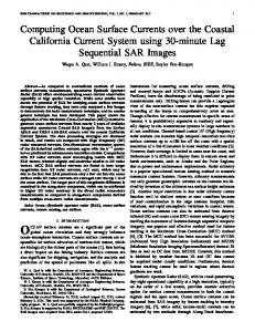
Fig. 1. MCC method. The solid box in the first image has been labeled as the “template subwindow”; this is the pattern to search for in the second image. The larger dashed box in the second image is called the “search window.”
accurately depict the seasonal cycle and represent similar current fields in space and time. Correlations, root mean square (rms) differences, and bias statistics are compared with previous MCC error estimates to determine the level of agreement between thermal and ocean color derived velocities. Finally, we present the increase in velocity vector coverage provided by the addition of ocean color MCC velocities. Past studies have applied the MCC method to a limited time series of ocean color data, and to our knowledge, this is the first comprehensive comparison that has been carried out between thermal and ocean color derived surface currents. II. MCC M ETHOD The MCC method [6], [9] is an automated procedure that calculates the displacement of small regions of patterns from one image to another. The procedure, illustrated in Fig. 1, cross correlates a template subwindow in an initial image with all possible subwindows of the same size that fall within the search window of a second image. The location of the subwindow in the second image that produces the highest cross correlation with the subwindow in the first image indicates the most likely displacement of that feature. The velocity vector is then calculated by dividing the displacement vector by the time separation between the two images. The main parameters controlling the MCC method are the minimum and maximum allowable time separation between images, the size of the template subwindow, and the size of the search window. The studies in [3] and [4] utilized thermal imagery and found that MCC velocities are most productively computed when the separation between images is less than 12 h. Ocean color images, however, are discretely separated by either 3–4 h or 21–27 h. In order to have enough velocity data points for this paper to be feasible, the use of a longer maximum time separation must be investigated. To do this, correlations were computed between thermal and ocean color velocities derived from image pairs with various time separations. This analysis is described in detail at the beginning of Section V and suggests that MCC currents can be consistently computed from time separations greater than 12 h. The size of the template subwindow is a balance between containing enough features for tracking (and hence having enough degrees of freedom for a statistically significant correlation) and smoothing out the structure of the flow. After comparing a number of velocity fields derived from various
template sizes, we determined that a 22 × 22 pixels (24.2 × 24.2 km) box best represented the motion seen in computer animations of sequential imagery. We also specified an overlap of 11 pixels between consecutive subwindows to increase the grid resolution to 11 × 11 pixels (12.1 × 12.1 km). The search window in the second image must be large enough to accommodate the largest expected velocity, which was specified as 70 cm/s for a number of reasons. The study in [10] indicates that high-velocity jets located off the California coast are characterized by core speeds that exceed 50 cm/s. After testing various maximum velocity thresholds, we found that the MCC method detected very few velocities greater than 70 cm/s and that a majority of these vectors were spatially incoherent. Velocities of this magnitude likely result from erroneous high correlations, as discussed in [1]. Minimizing the velocity threshold reduces the possibility of obtaining a high correlation by chance and decreases the MCC processing time. A raw MCC output velocity field contains vectors at every grid point, many of which result from low correlations. To capture vectors that accurately depict the ocean surface currents, the raw MCC vectors must be strictly filtered. The first filter employed is a correlation cutoff, which removes vectors that result from poorly correlated subwindows. As described in [1], the correlation cutoff value is increased with an increasing search range to reduce the possibility of obtaining a high correlation coefficient by chance. The second filter is a next-neighbor filter which removes spatially incoherent vectors. This filter requires that the immediate neighboring vectors surrounding a target vector agree to within a certain magnitude. For this paper, it is required that both the u and v components of three neighboring vectors are within 10 cm/s of the target vector components. After the filtering process is complete, the individual vector fields can be composited over a specified period of time to increase the spatial coverage and depict the mean flow. It is important to note that the composite vector field will represent the mean flow (or close to the mean flow) only if there is a consistent vector coverage throughout the compositing period. If the coverage is intermittent, the composite field will contain velocities from various times throughout the compositing period and could have a temporal bias. In this case, the composite field has improved spatial coverage, but does not represent the mean flow. Rather, it is simply a merged view of instantaneous velocities taken from different times during the compositing period. A number of past studies have analyzed the accuracy of the MCC method by comparing MCC velocities derived from thermal AVHRR imagery to independent current measurements. The study in [4] compared MCC currents to acoustic Doppler current profiler (ADCP) data and geostrophic velocities computed from dynamic height data and found rms difference errors on the order of 25 cm/s. The study in [5] processed 11 AVHRR images from a three-day period and suggested that MCC currents underestimate drifting buoy and ADCP currents by 30%–50% and have rms directional differences on the order of 60◦ . However, these differences were comparable to the differences between ADCP and drifting buoy currents. The study in [11] found the maximum correlation coefficient
CROCKER et al.: COMPUTING SURFACE CURRENTS FROM INFRARED AND OCEAN COLOR SATELLITE IMAGERY
437
between MCC and geostrophic currents to be 0.73. The study in [1] processed seven years of AVHRR data using the MCC method and compared the resulting currents with geostrophic currents computed from dynamic height data, satellite altimeter currents, and drifting buoy currents. They estimate the precision of the MCC method to be between 8 and 20 cm/s. These studies all conclude that the MCC method is an effective technique for determining the mesoscale surface flow. If the error between AVHRR and ocean color derived MCC velocities is within the range of error established by these past comparisons, it is strong evidence that AVHRR and ocean color MCC velocities can be merged together to increase the spatial and temporal coverage while maintaining the overall accuracy of the MCC method. III. S ATELLITE I MAGERY AND I NDIVIDUAL MCC V ELOCITY F IELDS In this section, we first describe the imagery that is used in this paper and the resulting individual surface velocity fields (“individual” refers to a postfiltered precomposited single vector field derived from two sequential images). Sample images and their corresponding vector fields are presented to illustrate how the addition of ocean color increases the overall vector coverage by reducing the effects of isothermal flow, clouds, and lack of satellite data. The vectors analyzed in this paper were derived from two separate sets of images located within the region 32◦ N to 42◦ N and -118◦ W to -132◦ W. The first set is a year-long collection of AVHRR thermal infrared (11 µm) images obtained from the National Oceanic and Atmospheric Administration (NOAA) 12, 16, and 17 polar-orbiting satellites in 2003. The study in [1] demonstrated that it is more effective to use 11-µm brightness temperature (BT) images than computed sea surface temperature (SST) images for the MCC application. This is due to the fact that the standard SST algorithm uses the difference between AVHRR channels 4 and 5 as part of the SST calculation, which has the effect of amplifying the noise in the resulting SST image. Cross correlations were found to be consistently higher if 11-µm BTs were used instead of an SST product. Since the MCC method computes velocities from feature displacements, precise image registration is essential since any errors in geolocation will be treated as surface displacements, producing errors in the estimates of the surface velocities. The images have been geolocated to an estimated 1-km pixel accuracy using the method described in [12]. AVHRR images are also cloud masked so that cloud motion is not detected by the MCC method. Nominally, six AVHRR thermal BT images were available per day (two images from each satellite). An example thermal image from October 27, 2003, is presented in Fig. 2 along with the vector field that was computed from the image shown and an AVHRR image acquired on the same day at 11: 00 GMT. The second set of images are chlorophyll_a concentrations from the Moderate Resolution Imaging Spectroradiometer (MODIS) (onboard the Aqua and Terra satellites) and Seaviewing Wide Field-of-view Sensor (SeaWiFS) (onboard the SeaStar satellite) ocean color sensors and were obtained from the Goddard Space Flight Center (GSFC) Distributed Active
Fig. 2. Channel 4 (11 µm) AVHRR image from October 27, 2003, at 22:24 GMT and MCC vectors derived from this image, and an AVHRR image acquired on October 27 at 11:00 GMT. Vectors in subregions A, B, and C are compared to those in Fig. 3 to illustrate the complementary nature of thermal and ocean color derived MCC velocities and how merging these two products increases the vector coverage. (Subregion A) The thermal-derived MCC vectors are located at the center and southwest edge of the rotating eddy feature. The thermal gradient along the upper edge of the feature is too weak to be tracked by the MCC method. (Subregion B) The number of MCC vectors is limited due to extensive cloud cover. (Subregion C) The MCC vectors are located along the northern and western edge of this region where there is a relatively strong thermal gradient.
Archive Center. This collection of ocean color imagery spans all of 2003 and covers the same geographic region as the AVHRR imagery. The 1.1-km-resolution MODIS ocean color data were converted to chlorophyll_a concentrations using the Chlor_a_2 algorithm [13]. The ∼1-km resolution data from the SeaWiFS instrument were converted to chlorophyll_a concentrations using the OC4 algorithm [14]. The MODIS and SeaWiFS data systems at the GSFC performed the geolocation and cloud masking of these images, which are accurate to within 1 km. Since ocean color images are only produced from daytime satellite imagery, nominally three images were available per day (one from each satellite). A sample ocean color image from October 26, 2003, is presented here in Fig. 3 along with the vector field that was derived from the image shown and a MODIS image acquired on the same day at 18:35 GMT. Figs. 2 and 3 depict some general characteristics of the thermal and ocean color imagery and illustrate the advantage of deriving surface currents from both image sets. A comparison between the images shown in Figs. 2 and 3 indicates that the large-scale surface features are similar; however, the details of these features are not the same, suggesting the complementary nature of the two MCC-derived velocity fields. The source of the infrared surface temperature patterns in this region is coastal upwelling [15] which creates cold tongues that become involved with local baroclinic instability processes, resulting
438
IEEE TRANSACTIONS ON GEOSCIENCE AND REMOTE SENSING, VOL. 45, NO. 2, FEBRUARY 2007
Fig. 3. Chlorophyll_a computed from MODIS ocean color data on October 26, 2003, at 21:50 GMT and MCC vectors derived from this image, and an ocean color image from October 26 at 18:35 GMT. (Subregion A) The ocean color derived velocities are located along the northern and western edge of the rotating eddy feature. The ocean color gradient is relatively weak in the center where MCC velocities are not present. (Subregion B) This region is cloud free in both ocean color images and facilitates extensive feature tracking as evidenced by the large number of MCC velocities. (Subregion C) The MCC velocities are not present because this region was beyond the edge-of-scan in the corresponding image acquired at 18:35 GMT.
in mesoscale eddies and their associated offshore directed tongues [16]. Chlorophyll surface patterns owe their existence to the biological activity in the study region. The same coastal upwelling that generates the cold tongues drives part of this activity, but other influences also contribute to the details of the ocean color surface patterns. The thermal and ocean color surface patterns evolve similarly over time, indicating that the forcing mechanisms responsible for the patterns are similar. It is evident that the surface currents advect the thermal and chlorophyll features in nearly the same manner, such that the thermal and ocean color features and their displacements have a high correspondence. For this reason, spatially coincident thermal and ocean color derived MCC velocities should correlate well in regions of large scale (relative to the MCC template subwindow size of 22 × 22 pixels) coherent flow, where features are advected linearly with minimal rotation and deformation. As an example, both thermal and ocean color vectors identify a southerly flowing jet located directly below subregion A in Figs. 2 and 3. It should be noted that the MCC method is capable of identifying largescale rotations, such as eddies, by tracking the differential linear translation of smaller features encompassed within the larger rotating feature. Ocean color features can complement thermal features, providing chlorophyll gradients where the thermal gradients are nonexistent or too weak to be tracked by the MCC method. One
Fig. 4. Combined thermal and ocean color vector fields from Figs. 2 and 3. The thermal vector field was derived from an image pair acquired on October 27, 2003, and the ocean color vector field was derived from an image pair acquired on October 26, 2003. Notice the complementary nature of the two independent velocity fields and how merging the two fields increase the coverage. (Subregion A) By merging the thermal and ocean color derived velocity fields, the eddy rotation is fully resolved. (Subregion B) Ocean color vectors provide significant coverage improvement due to a lack of cloud cover. (Subregion C) Thermal vectors provide surface-current information where ocean color data are lacking.
example of this can be seen in subregion A of Figs. 2 and 3. The thermal gradients along the northern and western edges of the eddy are quite diffuse, and the MCC method was unable to detect the feature displacements. However, the ocean color gradients sufficiently define these edges of the eddy, such that the MCC method is able to resolve the rotational flow. Conversely, thermal imagery can complement ocean color imagery. On the eastern side of the eddy, the MCC method was able to track the thermal features, but was unable to produce ocean color vectors due to weak gradients. Fig. 4 shows the two vector fields, with the thermal velocities in red and the ocean color velocities in black. Note that, the rotation in subregion A is clearly resolved in the combined velocity field, but unresolved in the separate fields. The effects of cloud cover and a lack of satellite coverage provide additional motivation for processing both thermal and ocean color imagery and merging the resulting vector fields. In Fig. 2, the ocean surface located within subregion B is almost completely obscured by clouds, resulting in very few vectors. This area is cloud free in the ocean color image pair, allowing the calculation of surface velocities. The MCC method did not track feature displacements in subregion C of Fig. 3 because this area was located beyond the edge-of-scan in the ocean color image acquired at 18:35 GMT. However, the two AVHRR images from October 27 contain data for this region, and the MCC method was able to calculate surface motion. Again, Fig. 4 shows both the thermal (red) and ocean color (black)
CROCKER et al.: COMPUTING SURFACE CURRENTS FROM INFRARED AND OCEAN COLOR SATELLITE IMAGERY
439
Fig. 5. Total number of MCC vectors per month in 2003 from (a) thermal AVHRR and (b) ocean color imagery. It should be noted that ocean color images are produced from daytime data only, while infrared images are collected during both day and night.
velocity fields and illustrates the increase in spatial coverage gained through the addition of ocean color derived vectors. The number of vectors in the thermal, ocean color, and combined fields are 533, 611, and 1021, respectively. For this one example, the addition of ocean color vectors increases the spatial coverage of thermal vectors by 92%. The maximum possible number of vectors in a single velocity field is 6213 when the grid spacing is 12.1 × 12.1 km. IV. V ELOCITY C OVERAGE The total number of thermal and ocean color MCC velocities computed each month in our study region is shown in Fig. 5. Due to the higher frequency of coverage provided by AVHRR imagery, there are considerably more thermal than ocean color velocities in almost every month of 2003. NOAA polar-orbiting satellites provide global coverage twice per day, one daytime image and one nighttime image. Since we used imagery from three NOAA satellites, there were approximately six thermal infrared AVHRR images available each day. The MODIS and SeaWiFS instruments also provide global coverage twice per day; however, ocean color images are only produced from data acquired during the daytime as visible channels are used in the algorithm. As a result, there were approximately three ocean color images available each day. The seasonal trend seen in the number of AVHRR and ocean color vectors is mainly a result of the cloud cover climatology of the study region, but is also influenced by the extent of trackable features. It is well known that fall has the clearest sky conditions off the coast of California, a fact which is clearly reflected by the high number of vectors during August through November. The spring of 2003 was a period of relatively high cloud cover, resulting in the low number of vectors surrounding April. The relatively large number of AVHRR vectors in mid summer is a bit of a surprise since summer in this region is often foggy and overcast due to the effects of coastal upwelling. To determine the monthly variability in the extent of trackable thermal and ocean color features, we normalize the Fig. 5 plots by their respective total annual number of vectors. There are a total of 187 858 thermal and 67 703 ocean color MCC velocities from 2003. The normalized plots, shown as Fig. 6,
Fig. 6. Monthly percent of the total number of thermal and ocean color MCC velocities in 2003.
depict the monthly percentage of the total number of vectors. Assuming that clouds have a relatively equal affect on the number of thermal and ocean color vectors on a monthly basis, differences between the thermal and ocean color monthly percentage of vectors will be due to differences in the extent of trackable features. During spring, there is a higher percentage of ocean color derived than thermal-derived velocities, corresponding to the spring phytoplankton bloom in the CC. The study in [17] analyzed approximately seven years of CZCS imagery from the CC region and found that chlorophyll concentrations reach their annual maximum from May to June; however, these high concentrations are located close to the coast. From March to May, the concentrations are not quite as high, but the chlorophyll is distributed over a much larger area offshore. This widespread distribution of chlorophyll corresponds to a large extent of trackable features, leading to the high percentage of ocean color MCC velocities found during spring. April appears to be somewhat of an anomaly during this period, but the reduction in the percentage of ocean color vectors during this month is likely due to extensive cloud cover. This is supported by the fact that the percentage of thermal vectors also decreases to a minimum. By June, the spring bloom has subsided, and there are more trackable thermal features than ocean color features. Fall is characterized by a minimal cloud cover and a second phytoplankton bloom [17], such that the percentage of thermal and ocean color vectors is nearly the same. Chlorophyll concentrations do not reach their annual maximum at this time, but there are significantly high concentrations throughout the extent of the study region that provide a large number of trackable features. Fig. 7 shows the spatial distribution of all thermal and ocean color derived vectors from 2003. The thermal vectors are distributed along the length of the California coast, with the largest number of vectors occurring near San Francisco Bay. The number of thermal vectors diminishes farther away from the coast, with the coverage being poor toward the western boundary of the study region. The ocean color vectors are
440
IEEE TRANSACTIONS ON GEOSCIENCE AND REMOTE SENSING, VOL. 45, NO. 2, FEBRUARY 2007
is advection by the surface currents. The offset locations of the most persistent trackable thermal and ocean color features hints at the advantage of combining the two MCC products. The high concentration of near-shore thermal-derived velocities is complemented by the high concentration of offshore ocean color derived velocities. V. C OMPARISONS OF M ONTHLY AND S EASONAL MCC V ELOCITY F IELDS A. Sampling Issues
Fig. 7. Spatial distribution of all (a) thermal and (b) ocean color derived vectors in 2003. For both plots, the lowest contour level is five vectors, such that grid points in the white areas may contain anywhere from zero to four vectors. The largest number of vectors occur in regions where the trackable surface features are most persistent. Note the different scales of the color bars.
concentrated along the southern California coast with the largest numbers occurring in the Southern California Bight. The ocean color vector coverage also decreases away from the coast and does not extend as far west as the thermal vector coverage. If we again assume that the spatial distribution of the clouds is relatively the same in the thermal and ocean color imagery throughout the year, it is evident that a majority of the trackable thermal features are located close to shore along the entire length of California, whereas the trackable ocean color features are concentrated slightly farther offshore. One possible explanation for this discrepancy is that nonadvective processes, such as biomass reproduction, may control the chlorophyll distribution along the inshore coastal region. Since the MCC method is only sensitive to advection, the ocean color derived velocities are concentrated slightly offshore where the dominant mechanism controlling the chlorophyll distribution
Ocean surface velocity vectors were computed using the MCC method for the cloud-free portions of image pairs separated by 3–31 h. Cloud cover, edge-of-scan distortions, lack of data, and regions of isothermal flow result in MCC velocity fields with highly variable spatial and temporal coverage. Compositing individual velocity fields increases the spatial coverage and improves the accuracy of MCC-derived velocities when compared to other surface current estimates [4], [11]. To accomplish this task and to accentuate the dominant mesoscale flow, we created monthly composites of thermal and ocean color MCC velocity fields for 2003. In order to assess the intrinsic correspondence between thermal and ocean color derived surface velocities, all the coincident velocities (coincident thermal and ocean color velocities are those that are located at the same grid location in a composite velocity field) from the twelve monthly composites are decomposed into their cross- and along-shore components. The positive along-shore direction is defined as 26 degrees west of North and the positive cross-shore direction is 26 degrees north of East. This coordinate system better represents the coastal geography and physical nature of the currents in the study region. As mentioned earlier, previous studies found that MCC velocities are most successfully computed when the separation between image pairs is less than 12 h. However, few ocean color images have time separations within that range, so that the maximum time separation was extended to 31 h. To determine the effect of the image time separation on the consistency of the thermal and ocean color MCC vectors, we calculated correlations between thermal and ocean color vectors for various time separations. Ocean color vectors were separated into two groups, vectors derived from image pairs with a time separation ranging from 3 to 4 h and vectors derived from images with a 21–27-h separation. The time separations of all ocean color image pairs fell in one of these two ranges. The distribution of time separations for AVHRR thermal image pairs was much more uniform, allowing the vectors to be divided into five groups corresponding to the following image time separations: 3–7, 7–12, 12–19, 19–25, and 25–31 h. Thermal and ocean color monthly composites were created for each respective time separation range, and correlation coefficients were calculated for all spatially coincident thermal and ocean color vectors. Fig. 8 summarizes these results and shows correlations as a function of thermal image time separation for the two ocean color time separations. The results are analyzed in terms of the thermal image time separations since they provide a sufficient temporal distribution from which the effects of image time separation can be examined.
CROCKER et al.: COMPUTING SURFACE CURRENTS FROM INFRARED AND OCEAN COLOR SATELLITE IMAGERY
Fig. 8. Correlation coefficients between coincident thermal and ocean color derived velocities in monthly composites as a function of image time separation. Correlations are computed for the cross- and along-shore velocity components. Ocean color imagery is discretely separated by 3–4 or 21–27 h, whereas the thermal imagery can be separated by 3–31 h. The 95% confidence interval is shown for each correlation coefficient.
Fig. 8 indicates that thermal and ocean color MCC velocities generally have the lowest correlations for the shortest (3–7 h) and longest (25–31 h) image time separations, while the highest correlations occur for intermediate time separations (7–25 h). Correlations may be low for short time separations because the effective resolution of the MCC method is proportional to the image time separation. The smallest velocity (a displacement of one pixel) that can be detected between images separated by 3 h is approximately 10 cm/s. The velocity resolution increases to approximately 1 cm/s for images separated by 31 h. This implies that the longer time separations have a greater sensitivity to feature displacements and potentially provide more precise velocity estimates. It is also clear that very long time separations do not provide consistent results. One possibility is that surface features deform or rotate significantly over long time periods, such that the MCC method is unable to accurately detect the feature displacements. Contrary to past studies, it is evident that the MCC method can produce consistent currents from imagery with time separations as large as 25 h. Although somewhat subjective, we suggest that image time separations less than 6 h and greater than 25 h should be neglected or used with caution. Preliminary qualitative analysis suggested that there was poor agreement between the low-velocity vectors. To investigate this, correlation coefficients were computed for coincident vectors falling within specified magnitude ranges. The six magnitude bins are: 0–5, 5–10, 10–20, 20–30, 30–40, and 40–50 cm/s. The correlation coefficients between ocean color and thermal vectors for each bin are shown in Fig. 9. It is clear that correlations are largest for high-velocity surface features, with correlations near 0.8 and higher for velocities ranging from 10–50 cm/s. The low-velocity thermal and ocean color vectors have poor agreement, with cross- and along-shore correlation coefficients of 0.08 and 0.10 for vectors ranging from 0–5 cm/s.
441
Fig. 9. Relationship between velocity magnitude and correlation coefficient for the cross- and along-shore components of coincident thermal and ocean color velocities in monthly composites. The 95% confidence interval is shown for each correlation value.
A majority of the low-velocity vectors are concentrated close to shore on the continental shelf (Fig. 10) where local topography, tides, upwelling, and other small-scale processes can have a large influence on the surface flow. The MCC method may have difficulty in accurately identifying low-magnitude surface currents for a number of reasons. Shelf circulation features often have time scales of one to three days and length scales of 3–10 km [18]. These scales are too fine to be resolved by monthly composites and the 24.2 × 24.2 km MCC template subwindow that was utilized for our computations. In addition, small image navigation errors can produce inaccurate low-magnitude vectors. A 1-km navigation error over 31 h (the longest time separation between images) corresponds to a velocity error of 0.90 cm/s, while the same navigation error over a 3-h time separation (shortest time between images) corresponds to a velocity error of 9.26 cm/s. The mean image miss-navigation velocity error is around 5 cm/s. A slight error in the AVHRR image geolocation causes the coastline to be offset in sequential images. The MCC method detects this coastal displacement and produces velocities over land. Land velocities are not produced from sequential ocean color imagery because land contaminated pixels were removed (set to zero) prior to our acquisition of the data. This fact ensures that land velocities are not included in the correlations computed between coincident thermal and ocean color derived velocities. We have masked out a majority of the thermal land vectors; however, the contours over land in Fig. 10(a) indicate that a few land vectors are still present [contours over land in Fig. 10(b) are simply a result of the plotting program]. To eliminate the few remaining land vectors and minimize the influence of weak inaccurate shelf velocities and imprecise image navigation, all velocities with magnitude less than 5 cm/s are removed and excluded from further comparison analysis. This method was also employed in [5], where vectors with magnitude less than 5 cm/s were removed from their MCC analysis to prevent a disproportionately large contribution to error differences from very small velocities.
442
IEEE TRANSACTIONS ON GEOSCIENCE AND REMOTE SENSING, VOL. 45, NO. 2, FEBRUARY 2007
Fig. 10. Location and number of (a) thermal and (b) ocean color velocities from monthly composites with magnitudes less than 5 cm/s. These velocities are removed from further analysis.
B. Seasonal Composite Velocity Fields The CC is generally characterized as a broad southeastward flow with significant seasonal variability. The study in [19] recently documented a representative seasonal cycle for the CC based on five years of altimeter-derived surfacecurrent residuals. The residual surface flow was computed from sea surface height anomaly data and represented the mean-removed geostrophic surface circulation. Their analysis suggests that the seasonal cycle begins in spring (April–June) with equatorward flow persisting directly offshore southern California. This southerly flow strengthens and propagates northwest as the surface currents weaken along the southern California coast. Surface velocities reach a maximum in the summer (July–September) and are strongest offshore northern California. The poleward Davidson current begins to develop along inshore regions of the California coast. During fall (October–December), the equatorward flow continues to propagate offshore and the Davidson current expands northward. A weakening of the southerly CC is found along the full extent of the California coast. By winter (January–March), the equa-
torward transport of the CC is significantly reduced, and the Davidson current reaches its maximum extent. At this time, the strongest surface currents are found offshore and to the south. This section focuses on comparing thermal and ocean color derived seasonal velocity composites to verify that these two MCC products represent similar velocities fields in space and time and accurately depict the characteristic seasonal cycle of the central CC. In Fig. 11(a)–(d), we present seasonal velocity composites derived from infrared imagery in red and those from the ocean color imagery in black. Our presentation begins in winter of 2003 to maintain the chronological order of our velocity dataset. The composite velocities are on a 24.2 × 24.2 km grid. They have been filtered using the next-neighbor filter, and velocities with magnitude less than 5 cm/s have been removed. The correlations and rms differences between the thermal and ocean color seasonal velocity composites are presented in Table I. These statistics are computed in the crossand along-shore directions for spatially coincident thermal and ocean color velocities in each seasonal composite. In winter [Fig. 11(a)], the largest MCC velocities occur offshore southern California, where significant eddy circulation remains from the previous seasonal cycle. Coastal velocities are quite weak, but exhibit a complex structure. The surface flow throughout the region is predominantly to the southeast. A poleward Davidson current is not evident. The surface currents are highly variable over the three-month winter composite period, suggesting an energetic culmination of the seasonal cycle. The jet that flows south along −127◦ W is prominent during January; however, by March, it flows eastward just north of 35◦ N. The agreement between coincident thermal and ocean color velocities is relatively poor, particularly in the offshore locations. The along- and cross-shore correlations are 0.50 and 0.67, and the rms differences are 10.47 and 10.09 cm/s, respectively. Disagreement between the thermal and ocean color MCC winter composites is attributed to minimal offshore sampling. As made evident by Fig. 7, very few MCC velocities are located in the southwest corner of the study region. The velocity coverage in this region was particularly poor during the winter months as a result of extensive cloud cover. The low sampling rate, in conjunction with the high-variability currents, produces a somewhat unreliable seasonal composite. Also, significant disagreement occurs between low-magnitude velocities and velocities located in the continental shelf region, as discussed in Section V-A. The thermal and ocean color derived spring seasonal composites [Fig. 11(b)] depict a broad equatorward meandering stream located adjacent to the southern California coast, corresponding to the beginning of the seasonal cycle. Offshore and to the north, the surface flow is slightly more complex and is dominated by shorter scale rotational features and narrow jets. While cloud cover also persists during the spring season, the coastal regions were sampled quite well and are now dominated by relatively high-velocity currents. The MCC method adequately detects the coastal surface flow, and the comparison statistics show a significant improvement compared to winter. The correlations have increased to 0.61 and 0.78, and the rms error has decreased to 6.61 and 6.51 cm/s in the along- and cross-shore directions.
CROCKER et al.: COMPUTING SURFACE CURRENTS FROM INFRARED AND OCEAN COLOR SATELLITE IMAGERY
443
Fig. 11. (a) Winter, (b) spring, (c) summer, and (d) fall 2003 seasonal velocity composites. Thermal-derived MCC velocities are shown in red and ocean color derived MCC velocities are shown in black. The orientation of the along- and cross-shore directions is shown in (c). TABLE I COMPARISON STATISTICS BETWEEN SPATIALLY COINCIDENT THERMAL AND OCEAN COLOR SEASONAL VELOCITY COMPOSITES FROM 2003. THE ORIENTATION OF THE ALONG- AND CROSS-SHORE DIRECTIONS IS SHOWN IN FIG. 11(c)
The inshore equatorward flow propagates west and north to create the strong summertime CC jet seen north of 35◦ N in Fig. 11(c). Compared to the spring season, the characteristic surface circulation has transitioned from a broad relatively weak southerly flow to a strong, narrow, highly dynamic jet that meanders east and west in a tight looping motion. While the structure of the jet has become more complex, the net flow of the jet continues to be in the southerly direction and
is well represented by both thermal and ocean color derived velocities. The equatorward flow weakens or reverses in the southern portion of the study region. The flow is predominantly offshore along the length of the California coast, corresponding to the strong upwelling conditions that exist during the summer in this region. The relatively cloud-free conditions and high surface velocities found during the summer of 2003 provide optimal conditions for the MCC method and lead to the high
444
IEEE TRANSACTIONS ON GEOSCIENCE AND REMOTE SENSING, VOL. 45, NO. 2, FEBRUARY 2007
Fig. 12. Mean along- and cross-shore velocities for thermal and ocean color seasonal composites. A positive cross-shore velocity indicates onshore flow and a positive along-shore velocity indicates northwesterly flow [see Fig. 11(c) for orientation].
correlations and low rms differences between the two MCC velocity products. The correlations are 0.81 and 0.82 in the along- and cross-shore directions, and the rms error reaches an annual minimum of 6.52 and 5.75 cm/s. By fall [Fig. 11(d)], the CC jet has moved slightly farther offshore and continues to increase in complexity. It is no longer a single meandering stream. A large loop in the jet has been severed from the main flow to form a cyclonic eddy centered at −129◦ W and 38◦ N. The circular eddy is clearly marked by a ring of red and black vectors surrounding the vector-free center. The centers of eddies are characterized by purely rotational, isothermal, and iso-color flow, which the MCC method is unable to detect. Both thermal and ocean color velocities depict a smaller anticyclonic eddy centered at −124◦ W and 35◦ N. This eddy appears to be interacting with the strong jet to the west of it, possibly causing a break in the southerly flow. A narrow poleward Davidson current located along the coast north of San Francisco Bay is clearly represented by both MCC products. Again, the clear fall skies provide ideal conditions for the application of the MCC method. As a result, the alongand cross-shore correlations peak at 0.84 and 0.89, and the rms error between the thermal and ocean color derived composites remains low at 6.56 and 6.47 cm/s. In Fig. 12, we present the mean along- and cross-shore velocities for the thermal and ocean color derived seasonal composites. As indicated by the orientation arrows in Fig. 11(c), a positive velocity in the cross-shore direction represents onshore flow, while a positive velocity in the along-shore direction represents northwesterly flow. In winter, the positive crossshore velocity corresponds to the transition of the CC jet from fall, where it is located far offshore, to spring, where the jet is located closest to the shore. From winter to spring, the along-shore velocity increases (becomes more negative) in the southerly direction, which correlates to the development and strengthening of the summertime jet. The cross-shore velocity is slightly negative during this time, indicating that the jet is beginning its progression offshore. During summer,
the equatorward flow weakens in the southern portion of the study region, which is reflected by the reduced magnitude of the southerly flow. The cross-shore flow, however, reaches its maximum velocity, corresponding to the strong summertime upwelling conditions. The cross-shore flow appears to force the summertime jet to the west as it begins to kink and meander back and forth in the east–west direction. These processes leads to the high cross-shore mean velocity seen in summer. The offshore propagation of the CC jet slows in fall as it approaches its farthest westward extent. The mean along-shore velocity stays relatively constant from summer to fall, indicating the transition into the next seasonal cycle. It is clear that both the thermal and ocean color derived seasonal composites accurately depict a majority of the seasonal cycle described in [19]; however, there is some disagreement during winter. The two MCC winter composites indicate relatively strong southerly flow throughout the study region, contrary to the weakened southerly or poleward flow suggested in [19]. The MCC method did not detect the poleward Davidson current during the winter of 2003, but it is evident in the fall 2003 velocity composite. With the exception of winter, the correlations between the two MCC products are close to or above the maximum correlation of 0.73 calculated in [11]. The rms differences are well below the average rms errors of 25 and 14 cm/s established in [1] and [4], and the mean bias between the two datasets is less than 2 cm/s (Fig. 12). It is interesting to note that the cross-shore correlations are consistently higher than those for the along-shore velocities. This suggests that the cross-shore velocities are more consistently captured by both the infrared and ocean color images. Likewise, the rms variability is greater for the along-shore component than it is for the cross shore, which may reflect the increased variability introduced by the combination of the mesoscale eddies and the predominately southward CC. The error between the thermal and ocean color MCC velocities is less than the established absolute error of the MCC method, suggesting that these independent current estimates can be merged together to form a refined current map without degrading the overall accuracy of the MCC method. VI. I NCREASED V ECTOR C OVERAGE The previous sections established the high correspondence between thermal and ocean color derived velocities. The present section will address the increase in velocity coverage that results from the combination of the two MCC products. To illustrate the increase in vector coverage provided by ocean color, we examine the temporal and spatial distribution of the coverage increase. Fig. 13 shows the percent increase in the total number of vectors provided by ocean color for each month in 2003. The addition of ocean color increases the total number of MCC vectors between 10% and 110%, depending on the month, with an average increase around 40%. It is important to recall that there was approximately twice the number of thermal images processed as ocean color images, suggesting that the 40% increase provided by ocean color represents a significant number of vectors. It should be noted that some of the ocean color derived velocities will occur at the same locations as the
CROCKER et al.: COMPUTING SURFACE CURRENTS FROM INFRARED AND OCEAN COLOR SATELLITE IMAGERY
Fig. 13. Percent increase in the total number of MCC vectors provided by the addition of ocean color for each month in 2003.
thermal-derived velocities and therefore will not provide new data. However, since the two MCC products are independent and have a high agreement, merging coincident thermal and ocean color velocities increases the statistical significance of the resulting velocity estimate. To evaluate the increase in spatial coverage (the amount of new data) provided by ocean color vectors, we compare the number of spatially noncoincident ocean color vectors to the total number of thermal vectors at each grid point in threeday composites. The relatively short compositing period of three days was used for this purpose to obtain a more accurate representation of the instantaneous spatial variability, free from the compositing effects (filling in gaps in vector coverage) associated with longer period composites. Thermal and ocean color three-day composites were created for all of 2003, and the spatially noncoincident ocean color vectors were identified. The percent increase in vector coverage provided by ocean color was calculated by dividing the number of noncoincident ocean color vectors at each grid point by the total number of thermal vectors at each grid point. Fig. 14 shows the percent increase in spatial vector coverage (synonymous to the percent increase in new data) in three-day composites provided by ocean color. The addition of ocean color increases the coverage anywhere from 0%–100+%, with an average increase of approximately 25%. It is now evident that ocean color MCC velocities provide a significant number of reliable surface-current estimates, where thermal velocities are not present, and the two MCC products can be merged together to form a refined surface-current map with enhanced coverage and statistical significance. VII. S UMMARY D ISCUSSION The MCC method is an automated technique that can be implemented to calculate feature displacements between two sequential images. Numerous studies have applied this method to AVHRR thermal infrared imagery and have cited its capabilities in mapping advective ocean surface currents. Comparisons with in situ and other remotely sensed current measurements suggest that MCC-derived velocities have rms magnitude dif-
445
Fig. 14. Spatial increase in vector coverage in three-day composites provided by ocean color. This illustrates that ocean color adds a significant number of new surface-current estimates where thermal-derived velocities are not present.
ferences on the order of 10–20 cm/s, with correlations around 0.70 [1], [4], [5], [11]. While the MCC method is constrained to the detection of linear advection with minimal deformation, it is also limited by cloud cover, undesirable satellite viewing conditions, and isothermal flow. These characteristics result in velocity fields with highly variable spatial and temporal coverage. The intention of this paper was to determine if surface currents could be consistently calculated from sequential ocean color imagery and to evaluate the degree at which these velocities correspond to MCC velocities derived from thermal imagery. If the thermal and ocean color derived velocities agree to within the established absolute error of the MCC method, it is a strong evidence that the two products can be merged together to increase the overall coverage of the resulting velocity fields. While it is true that any additional source of imagery would increase the sampling rate of the ocean surface and thereby increase the number of MCC-derived velocities, two independent velocity products should not be merged unless they depict very similar circulation. Ocean color imagery has the same resolution as AVHRR imagery and is, therefore, a likely source of supplemental MCC velocities. In this analysis, MCC surface currents are derived from yearlong collections (2003) of 1.1-km-resolution AVHRR thermal infrared imagery and 1.1-km MODIS and SeaWiFS ocean color imagery for the central CC. Examination of individual image pairs and the corresponding velocity fields indicates the complementary nature of these two datasets and the velocities derived from them. It is evident that the MCC method can detect ocean color feature displacements in regions of isothermal flow and vice versa, which leads to a spatial and temporal increase in vector coverage. While the ocean color signal is also attenuated by clouds, processing this dataset, in addition to thermal imagery, increases the sampling of the ocean surface, thus reducing the effects of undesirable viewing conditions and isothermal flow. Monthly composites were created to analyze the correspondence between thermal and ocean color derived velocities. Contrary to past recommendations [3], [4], we found that MCC
446
IEEE TRANSACTIONS ON GEOSCIENCE AND REMOTE SENSING, VOL. 45, NO. 2, FEBRUARY 2007
velocities can be effectively calculated from image pairs with time separations on the order of one day. The agreement between thermal and ocean color was relatively high for MCC velocities derived from image pairs with time separations between 7 and 25 h and was significantly lower for velocities derived from image pairs with time separations outside of this range. Correlations were below 0.10 between spatially coincident velocities with magnitude less than 5 cm/s. These low-magnitude vectors were concentrated close to the coast, suggesting that the MCC method does not adequately detect the short space and time scale processes that can dominate the continental shelf region. In addition, small errors in image geolocation translate into velocity errors on the order of 5 cm/s, limiting the reliability of low-magnitude MCC velocities. On the other hand, velocities greater than 10 cm/s had correlations higher than 0.8, indicating the consistent detection of high velocity flow by the thermal and ocean color MCC products. The correlations between coincident thermal and ocean color velocities (with magnitudes greater than 5 cm/s) from seasonal composites range from 0.50 to 0.89, with a mean correlation of approximately 0.74. The mean rms difference is approximately 7.4 cm/s, with a mean bias less than 2 cm/s. These difference statistics fall well within the established range of absolute MCC error calculated from previous studies (discussed at the beginning of this section). Both the thermal and ocean color derived seasonal velocity composites depict the major features of the CC seasonal cycle, confirming that these two products represent similar current fields in both space and time. For this specific case study, merging ocean color with thermal MCC velocities increases the total number of velocity estimates by approximately 40%, which provides around 25% new velocity data that are spatially noncoincident with the thermal MCC data. Sequential ocean color imagery is a reliable source for deriving surface-current estimates that complement thermalderived MCC velocities and can provide velocity information where thermal imagery does not permit feature tracking, such as regions of isothermal flow.
[6] W. J. Emery, A. C. Thomas, M. J. Collins, W. R. Crawford, and D. L. Mackas, “An objective method for computing advective surface velocities from sequential infrared satellite images,” J. Geophys. Res., vol. 91, no. C11, pp. 12 865–12 878, 1986. [7] J. F. R. Gower, K. L. Denman, and R. J. Holyer, “Phytoplankton patchiness indicates the fluctuation spectrum of mesoscale oceanic structure,” Nature, vol. 288, no. 5787, pp. 157–159, 1980. [8] C. A. E. Garcia and I. S. Robinson, “Sea surface velocities in shallow seas extracted from sequential coastal zone color scanner satellite data,” J. Geophys. Res., vol. 94, no. C9, pp. 12 681–12 692, 1989. [9] R. M. Ninnis, W. J. Emery, and M. J. Collins, “Automated extraction of pack ice motion from Advanced Very High Resolution Radiometry,” J. Geophys. Res., vol. 91, no. 10, pp. 725–734, 1986. [10] B. M. Hickey, “Coastal oceanography of Western North America from the tip of Baja California to Vancouver Island,” in In the Sea, vol. II, A. Robinson and K. Brink, Eds. Hoboken, NJ: Wiley, 1998. [11] J. Gao and M. B. Lythe, “Effectiveness of the MCC method in detecting oceanic circulation patterns at a local scale from sequential AVHRR images,” Photogramm. Eng. Remote Sens., vol. 64, no. 4, pp. 301–308, 1998. [12] W. J. Emery, D. Baldwin, and D. K. Matthews, “Maximum cross correlation automatic satellite image navigation and attitude corrections for open ocean image navigation,” IEEE Trans. Geosci. Remote Sens., vol. 41, no. 1, pp. 33–42, Jan. 2003. [13] K. L. Carder, F. R. Chen, Z. Lee, S. K. Hawes, and J. P. Cannizzaro, MODIS Ocean Science Team Algorithm Theoretical Basis Document. Greenbelt, MD: Goddard Space Flight Center, 2003. ATBD 19, Case 2, Chlorophyll_a. [14] J. E. O’Reilly, S. Maritorena, B. G. Mitchell, D. A. Siegel, K. L. Carder, S. A. Garver, M. Kahru, and C. McClain, “Ocean color chlorophyll algorithms for SeaWIFS,” J. Geophys. Res., vol. 103, no. C11, pp. 24 937– 24 953, 1998. [15] M. Ikeda and W. J. Emery, “A continental shelf upwelling event off Vancouver Island as revealed by satellite infrared imager,” J. Mar. Res., vol. 42, no. 2, pp. 303–317, 1984. [16] M. Ikeda, W. J. Emery, and L. A. Mysak, “Seasonal variability of the meanders in the California current system off Vancouver Island,” J. Geophys. Res., vol. 89, no. C7, pp. 3487–3505, 1984. [17] A. C. Thomas, F. Huang, P. T. Strub, and C. James, “Comparisons of the seasonal and interannual variability of phytoplankton pigment concentrations in the Peru and Californian current systems,” J. Geophys. Res., vol. 99, no. C4, pp. 7355–7370, 1994. [18] P. Marchesiello, J. C. McWilliams, and A. Shchepetkin, “Equilibrium structure and dynamics of the California current system,” J. Phys. Oceanogr., vol. 23, no. 4, pp. 753–783, 2003. [19] P. T. Strub and C. James, “Altimeter-derived surface circulation in the large-scale NE Pacific Gyres. Part 1. Seasonal variability,” Prog. Oceanogr., vol. 53, pp. 163–183, 2002.
ACKNOWLEDGMENT The authors would like to thank the program manager, E. Lindstrom, for the continued support and the reviewers for their useful comments. R EFERENCES [1] M. M. Bowen, W. J. Emery, J. Wilken, P. C. Tildesley, I. J. Barton, and R. Knewtson, “Extracting multi-year surface currents from sequential thermal imagery using the maximum cross correlation technique,” J. Atmos. Ocean. Technol., vol. 19, no. 10, pp. 1665–1676, 2002. [2] M. M. Bowen, J. L. Wilkin, and W. J. Emery, “Variability and forcing of the East Australian current,” J. Geophys. Res., vol. 110, no. C3, C03019, 2005. [3] W. J. Emery, C. Fowler, and A. Clayson, “Satellite-image-derived Gulf Stream currents compared with numerical model results,” J. Atmos. Ocean. Technol., vol. 9, no. 3, pp. 286–304, 1992. [4] R. Tokmakian, T. P. Strub, and J. McClean-Padman, “Evaluation of the maximum cross-correlation method of estimating sea surface velocities from sequential satellite images,” J. Atmos. Ocean. Technol., vol. 7, no. 6, pp. 852–865, 1990. [5] K. A. Kelly and P. T. Strub, “Comparison of velocity estimates from Advanced Very High Resolution Radiometer in the coastal transition zone,” J. Geophys. Res., vol. 97, no. C6, pp. 9653–9668, 1992.
R. Ian Crocker received the B.S. degree in environmental engineering from the University of Colorado, Boulder, in 2004, where he is currently working toward the M.S. degree in aerospace engineering sciences. He is currently a Research Assistant with the Colorado Center for Astrodynamics Research, University of Colorado. His research involves various remote-sensing applications in physical oceanography.
Dax K. Matthews received the B.S. and M.S. degrees in aerospace engineering from the University of Colorado, Boulder, in 2002 and 2003, respectively, where he is currently working toward the Ph.D. degree in aerospace engineering. His primary research interest is satellite oceanography. He has also conducted research in space habitat design.
CROCKER et al.: COMPUTING SURFACE CURRENTS FROM INFRARED AND OCEAN COLOR SATELLITE IMAGERY
William J. Emery (M’90–SM’01–F’03) received the Ph.D. degree in physical oceanography from the University of Hawaii at Manoa, Honolulu, in 1975. After working at Texas A&M University, he moved to the University of British Columbia in 1978, where he created a satellite oceanography facility and educational program. He was appointed Full Professor in aerospace engineering sciences, University of Colorado, Boulder, in 1987. He is a coauthor of two textbooks on physical oceanography, has translated three oceanographic books (German to English), and has authored over 130 refereed publications. He is active in the analysis of satellite data for oceanography, meteorology, and terrestrial vegetation. His research interests are satellite sensing of sea surface temperature, mapping ocean surface currents, and terrestrial vegetation. He has recently started working in urban change detection using high-resolution optical imagery and synthetic aperture radar data. He also works with passive microwave data for polar applications to ice motion and ice concentration as well as atmospheric water vapor studies. In addition, his group writes analysis software and has established/operated data systems for the distribution of satellite data received by their own antennas. He is an Associate Member of the Laboratory for Atmospheric and Space Physics, an affiliate member of NOAA’s Cooperative Institute for Research in Earth Science, and a founding member of the University of Colorado’s Program in Atmospheric and Oceanic Sciences. Dr. Emery is a member of the Administrative Committee of the IEEE Geoscience and Remote Sensing Society and the Editor of the IEEE GEOSCIENCE AND REMOTE SENSING LETTERS.
447
Daniel G. Baldwin received the B.S. and M.S. degrees from Pennsylvania State University, University Park, in 1980 and 1983, respectively. From 1982 to 1988, he was an Associate Scientist with the National Center for Atmospheric Research, Boulder, CO, where he was involved in developing cloud detection algorithms for use with AVHRR data. From 1988 to 1993, he was a Senior Scientific Programmer with the Colorado Center for Astrodynamics Research, (CCAR), University of Colorado, Boulder. Since 1993, he has been a Senior Professional Research Assistant with CCAR, working on projects involving AVHRR data.