Computing the Radius of Pointedness of a Convex Cone - IMPA

Mathematical Programming manuscript No. (will be inserted by the editor) Alfredo Iusem · Alberto Seeger

Computing the Radius of Pointedness of a Convex Cone Dedicated to C. Gonzaga on his 60th Birthday Received: date / Revised version: date Abstract. Let Ξ(H) denote the set of all nonzero closed convex cones in a finite dimensional Hilbert space H. Consider this set equipped with the bounded Pompeiu-Hausdorff metric δ. The collection of all pointed cones forms an open set in the metric space (Ξ(H), δ). One possible way of measuring the degree of pointedness of a cone K is by evaluating the distance from K to the set of all nonpointed cones. The number ρ(K) obtained in this way is called the radius of pointedness of the cone K. The evaluation of this number is, in general, a very cumbersome task. In this note, we derive a simple formula for computing ρ(K), and we propose also a method for constructing a nonpointed cone at minimal distance from K. Our results apply to any cone K whose maximal angle does not exceed 120 degrees.

1. Introduction Let H be a real Hilbert space with inner product h·, ·i and associated norm k · k. Throughout this work, we assume that 2 ≤ dim H < ∞. A convex cone in H is understood as a nonempty set K ⊂ H satisfying tK ⊂ K for any t > 0 and K + K ⊂ K. The zero cone {0} is of no interest, and therefore it is left aside from the discussion. The set Ξ(H) = {K ⊂ H : K is a nonzero closed convex cone} is equipped with the bounded Pompeiu-Hausdorff metric δ(K1 , K2 ) = sup |dist[z, K1 ] − dist[z, K2 ]|,

(1)

kzk ≤1

where dist[z, K] stands for the distance from z to K. It is known (see e.g. [9]) that an equivalent expression for δ is given by   δ(K1 , K2 ) = max sup dist[z, K2 ], sup dist[z, K1 ] , (2) z∈K1 ∩SH

z∈K2 ∩SH

where SH denotes the unit sphere in H. Alfredo Iusem: Instituto de Matematica Pura e Aplicada, Estrada Dona Castorina 110 - Jardim Botanico, Rio de Janeiro, Brazil Alberto Seeger: University of Avignon, Department of Mathematics, 33, rue Louis Pasteur, 84000 Avignon, France Mathematics Subject Classification (1991): 47L07, 52A20

2

Alfredo Iusem, Alberto Seeger

Recall that a cone K ∈ Ξ(H) is said to be pointed if K ∩ −K = {0}. As shown in [3], the set P(H) = {K ∈ Ξ(H) : K is pointed} is open in the metric space (Ξ(H), δ). In order to measure the degree of pointedness of a cone K, the number ρ(K) =

inf

δ(Q, K),

(3)

Q∈M(H)

that is to say, the distance from K to the set M(H) = {Q ∈ Ξ(H) : Q is not pointed}, has been suggested in [4]. Since M(H) is compact in the metric space (Ξ(H), δ), the infimum in (3) is actually attained. The number ρ(K) is called the radius of pointedness of K because ρ(K) = sup{r ∈ [0, 1] : Ur (K) ⊂ P(H)} corresponds to the radius of the largest ball Ur (K) = {Q ∈ Ξ(H) : δ(Q, K) < r} centered at K and contained in P(H). The theoretical properties of the function ρ : Ξ(H) → [0, 1] are discussed in [4]. What worries us here is that the evaluation of ρ(K), using either (1) or (2), is, in general, a quite difficult task. Notice that the minimization variable in (3) is not a usual vector, but an element living in a metric space. The purpose of this paper is twofold: firstly, to derive a simple formula for evaluating ρ(K); and, secondly, to construct a nonpointed cone at minimal distance from K. Denote by θmax (K) the maximal angle that can be formed by picking up two unit vectors in K ∈ Ξ(H), that is to say, θmax (K) =

sup

arccos hu, vi.

(4)

u,v∈K∩SH

In constrast with (3), the above maximization problem takes place in a space having a linear structure. We assume that evaluating θmax (K) is not too expensive an operation or, at least, it is not as costly as evaluating ρ(K). Necessary optimality conditions for the nonconvex optimization problem (4) are derived in [5]. It is now well understood how to exploit these optimality conditions, for instance, in the case of a polyhedral cone. As we shall see in a moment, the term θmax (K) plays an important role in the discussion. Among other things, it appears in the very definition of the coefficient r   1 + cos θmax (K) θmax (K) = cos . (5) σ(K) = 2 2

Computing the Radius of Pointedness of a Convex Cone

3

The term inside the square root is called the angular index of K. It ranges over the closed interval [0, 1], taking the value 0 when K is not pointed and the value 1 when K is a ray. A more detailed explanation on the expression (5) could be helpful at this point in time, but, without further ado, we simply state: Theorem 1. Assume that K ∈ Ξ(H) is not a ray. Let K be moderate in the sense that θmax (K) ≤ 2π/3. Then, the following two conclusions hold: (a) ρ(K) is equal to σ(K), (b) if u, v ∈ K ∩ SH are such that arccos hu, vi = θmax (K), then K + R(u − v) is a member of M(H) lying at minimal distance from K. That a cone is moderate simply means that its maximal angle does not exceed 120 degrees. The reader may rightfully wonder why this special upper bound comes into the picture. We hope to provide at least a partial answer to this question by the end of this paper. Theorem 1 is our main result. Its proof is far from being a trivial exercise, and, unfortunately, we must go over a long series of preliminary lemmas.

2. Link to Mathematical Programming Although this paper deals exclusively with the relation between two measures of pointedness of a closed and convex cone, namely ρ(K) and σ(K), it is worthwhile to emphasize that it is part of an ongoing research project dealing with all measures of pointedness (cf. [4–6]). A general analysis of such measures has been undertaken in [6], where it is shown that any measure of pointedness evaluated at the dual cone K + = {y ∈ H : hx, yi ≥ 0 ∀x ∈ K} provides an adequate measure of solidity of K. Measures or indices of solidity play a meaningful role in the complexity analysis of interior methods for convex programming with conic constraints, as we describe next. Consider the problem minimize f (x) Ax = b, x ∈ K, where f : Rn → R is a convex and continuously differentiable function, A is an n × m real matrix, b is a vector in Rm , and K ⊂ Rn is a closed convex cone with nonempty interior. Generally speaking, these interior point methods execute Newton steps for minimizing the sum of the objective f plus a barrier function, subject just to the linear equality constraints. Thus, the iterate xk+1 is obtained by taking a Newton step from xk , for the penalized objective f (x) + ηk ϕ(x), subject to Ax = b. The terms ηk > 0 are penalization parameter and the barrier function ϕ : int(K) → R forces the sequence to stay in the interior of K, because it diverges to infinity when its argument approaches the boundary of K. A careful choice of the parameters ηk and the barrier function ϕ makes it possible to obtain accurate estimates of the number of iterations required to achieve an

4

Alfredo Iusem, Alberto Seeger

iterate xk whose distance to the solution set does not exceed a certain value ε (such number is called the computational complexity of the algorithm), and in fact such complexity is bounded by a low degree polynomial in log(1/ε). One of the conditions on ϕ, necessary for this kind of result, demands that it be conically log-homogeneous, i.e. such that ϕ(tx) = ϕ(x) + θ log t for all x ∈ K, all t > 0 and some θ > 0, and in this case the complexity includes a term of the order of log(1/θ). It turns out to be the case that the log-homogeneity constant θ of the barrier function is essentially an index of solidity of K, as considered in [6]. The most frequent solidity index of a cone K, used in the analysis of log-homogeneous barriers, is the Frobenius one, namely Fr(K) =



radius of the largest ball contained in K and centered in a unit vector.

It has been shown in [6] that Fr(K) = f? (K + ), where f? (K) denotes the basic index of pointedness of K, defined as the distance from the origin to the convex hull of the intersection of K with the unit sphere. Thus, indices of pointedness are of interest for determining the computational complexity ot these interior point methods. Since indices of solidity and of pointedness are essentially equivalent, via dualization, an in-depth study of indices of pointedness of cones is very likely have interesting consequences for the complexity theory of interior point algorithms. See e.g. [1] and [8] for the use of solidity indices in this context.

3. An equivalent expression for σ(K) In this section we exhibit an equivalent formulation for σ(K). We start by recalling the celebrated orthogonal decomposition lemma established by Moreau in 1962. We use the notation πK (z) to indicate the projection of z ∈ H onto K, that is to say, πK (z) is defined as the point in K at the shortest distance from z. As usual, K − = −K + stands for the polar (or negative dual) cone of K. Lemma 1. Consider a closed convex cone K ⊂ H and its polar K − . Each z ∈ H admits a unique decomposition in the form z = x + y, with x ∈ K, y ∈ K − , hx, yi = 0. In fact, x = πK (z) and y = πK − (z). Proof. See [2] or [7].

t u

Next we present a purely technical trigonometrical lemma. Lemma 2. For α ∈ [0, π/2] and β ∈ [π/2, π], it holds that cos(β − α) ≤ 1 − 2 min{cos2 α, cos2 β}.

(6)

Equality in (6) occurs exactly when α + β = π (or, equivalently, when cos2 α = cos2 β).

Computing the Radius of Pointedness of a Convex Cone

5

Proof. The inequality (6) can be rewritten in the form min{cos2 α, cos2 β} ≤ sin2 [(β − α)/2]. Assume, on the contrary, that cos2 α > sin2 [(β − α)/2]

and

cos2 β > sin2 [(β − α)/2].

(7)

Note that (β − α)/2 ∈ [0, π/2]. The first inequality in (7) yields sin[(β − α)/2] < cos α = sin[π/2 − α], from where it follows that α + β < π. Similarly, the second inequality in (7) yields sin[(β − α)/2] < − cos β = sin[β − π/2], from where we obtain π < α + β. In other words, both inequalities in (7) cannot occur simultaneously. The second part of the lemma is implicit in the above discussion. t u Define, for K ∈ Ξ(H), the minmax coefficient ξ(K) = inf max{dist[z, K], dist[−z, K]}. kzk=1

(8)

By combining Lemmas 1 and 2, we get: Proposition 1. For any K ∈ Ξ(H), it holds that σ(K) ≤ ξ(K). Proof. Suppose that K is not a ray, otherwise the result is trivial. Let z ∈ H be a unit vector such that ξ(K) = max {dist[z, K], dist[−z, K]},

(9)

i.e., z ∈ SH achieves the infimum in (8). For convenience, we write (9) in the form ξ(K) = max {kz − πK (z)k, k − z − πK (−z)k}. If πK (z) = 0, then kz − πK (z)k = 1 and ξ(K) = 1. Similarly, if πK (−z) = 0, then k − z − πK (−z)k = 1, and we get again ξ(K) = 1. In both cases, the result is trivial. So, without loss of generality, we assume that πK (z) 6= 0

and πK (−z) 6= 0.

This assumption is compatible with the fact that K is not a ray. We claim that [ξ(K)]2 ≥

1 1 + hx, yi, 2 2

(10)

with x = kπK (z)k−1 πK (z) and y = kπK (−z)k−1 πK (−z). From Lemma 1, we obtain hz, xi = kπK (z)k and hz, yi = −kπK (−z)k. So, it is rather trivial to prove that kz − πK (z)k2 = kz − hz, xixk2 = 1 − hz, xi2 ,

6

Alfredo Iusem, Alberto Seeger

k − z − πK (−z)k2 = k − z − h−z, yiyk2 = 1 − hz, yi2 . This yields the equality   [ξ(K)]2 = max 1 − hz, xi2 , 1 − hz, yi2 = 1 − min hz, xi2 , hz, yi2 . Since hz, xi ∈]0, 1[ and hz, yi ∈] − 1, 0[, one has α = arccoshz, xi ∈]0, π/2[ and β = arccoshz, yi ∈]π/2, π[. The use of Lemma 2 produces  1 − cos(β − α)  1 1  [ξ(K)]2 = 1 − min cos2 α, cos2 β ≥ 1 − = + cos(β − α). 2 2 2 For proving (10), we must verify that cos(β − α) ≥ hx, yi. With this purpose, we introduce the vectors 1 1 b= [x − (cos α)z], c = [y − (cos β)z]. sin α sin β By construction, b and c are unit vectors orthogonal to z. Hence, hx, yi = cos α cos β + sin α sin β hb, ci. Since α, β ∈]0, π[, one has sin α sin β ≥ 0, and therefore hx, yi ≤ cos α cos β + sin α sin βkbk kck = cos α cos β + sin α sin β = cos(β − α). This completes the proof of (10). Let θ= arccos hx, yi. From (10) and (5) we obtain r r 1 + cos θ 1 + cos θmax (K) ξ(K) ≥ ≥ = σ(K). 2 2 t u Before establishing the reverse inequality to that of Proposition 1, we present a few additional auxiliary results. The next lemma is elementary and has to do with the angular index of a finitely generated cone K = {Ga : a ∈ Rm + },

with Ga = a1 g1 + · · · + am gm .

(11)

The finite collection {g1 , · · · , gm } ⊂ H of nonzero vectors is called a set of generators for K. Notice that the variational problem minimize {hu, vi : u, v ∈ K ∩ SH } takes here the particular form  2 2 minimize hGa, Gbi : a, b ∈ Rm + , kGak = kGbk = 1 .

(12)

Lemma 3. Let K ∈ Ξ(H) be the cone generated by {g1 , . . . , gm } ⊂ H. Let (¯ a, ¯b) be a solution to the minimization problem (12). Then,  ¯ − (¯ at M ¯b)M ¯b ∈ Rm  +  Ma  ¯ M b − (¯ at M ¯b)M a ¯ ∈ Rm + (13) t a ¯ M a ¯ = 1    ¯t ¯ b M b = 1, where M denotes the m × m-matrix with entries hgi , gj i (1 ≤ i, j ≤ m).

Computing the Radius of Pointedness of a Convex Cone

7

Proof. A simple rearrangement of (12) tells us that the pair (¯ a, ¯b) solves also the following problem: min − (a − b)t M (a − b) (14) m s.t. at M a = 1, bt M b = 1, a ∈ Rm + , b ∈ R+ .

(15)

Thus, (¯ a, ¯b) satisfies the Karush-Kuhn-Tucker optimality conditions for (14)– (15), namely (15) and additionally M (¯b − a ¯ ) − λ1 M a ¯ ∈ Rm +, ¯ ¯ M (¯ a − b) − λ2 M b ∈ Rm , +

a ¯t [M (¯b − a ¯ ) − λ1 M a ¯] = 0, t ¯b [M (¯ a − ¯b) − λ2 M ¯b] = 0, for suitable KKT multipliers λ1 , λ2 ∈ R. By combining all these conditions, one gets λ1 = λ2 = a ¯t M ¯b − 1. By plugging this into the above system, one arrives at the desired conclusion. t u Remark: Notice that the conditions (13) are necessary for solving the minimization problem (14)–(15), but they are far from being sufficient. In fact, we are minimizing a function which is concave, not convex, and the feasible set is not convex either. The next result is also related to finitely generated cones. If K admits the representation (11), then the linear space spanned by K is simply the linear space spanned by the gj ’s. In short, spanK = span{g1 , · · · , gm }.

(16)

Imagine that we have a z in (16), and we want to project this vector onto the cone K. The following lemma helps us to compute such projection πK (z). Lemma 4. Let K ∈ Ξ(H) be the cone generated by {g1 , . . . , gm } ⊂ H, and M be the m × m- matrix with entries hgi , gj i (1 ≤ i, j ≤ m). Take any z = G(¯ ν ) with ν¯ ∈ Rm . Then, G(¯ µ) is the projection of z onto K if and only if, the complementarity system µ ¯ ∈ Rm µ − ν¯) ∈ Rm ¯t M (¯ µ − ν¯) = 0 + , M (¯ +, µ

(17)

holds. Proof. Clearly G(¯ µ) = πK (z) if and only if µ ¯ minimizes the function µ ∈ Rm 7→ kG(µ) − G(¯ ν )k2 over the positive orthant Rm + . This is a convex minimization problem which satisfies usual constraint qualifications, so that the Karush-Kuhn-Tucker conditions are both necessary and sufficient for optimality. These conditions are precisely those stated in (17). t u

8

Alfredo Iusem, Alberto Seeger

We now return to the case of a general cone K ∈ Ξ(H), and pick up the main stream of the discussion. Proposition 2. Take any K ∈ Ξ(H). For u, v ∈ K ∩ SH , the following two conditions are equivalent: (a) arcoshu, vi = θmax (K), (b) ku − vk = diam(K ∩ SH ). If u, v ∈ K ∩ SH satisfies any of these conditions, then πK (u − v) = (1 − hu, vi)u

and

πK (v − u) = (1 − hu, vi)v.

(18)

Proof. The equivalence between (a) and (b) is evident. Let us check the conclusion (18). If K happens to be a ray, then (18) holds trivially. So, we assume that u 6= v. We carry out the proof in two steps. Step 1. We suppose first that K is finitely generated. Consider the representation (11), and write u = G(¯ a), v = G(¯b), with a ¯, ¯b ∈ Rm + . In such a case u − v = G(¯ ν ),

with ν¯ = a ¯ − ¯b ∈ Rm ,

and also (1 − hu, vi)u = G(¯ µ),

with µ ¯ = (1 − hu, vi)¯ a = (1 − a ¯t M ¯b)¯ a.

In view of Lemma 4, in order to verify that πK (u − v) = (1 − hu, vi)u, it suffices to check that (¯ µ, ν¯) satisfies the complementarity system (17). First of all, one has hu, vi ≤ kukkvk = 1, and therefore µ ¯ ∈ Rm + . Secondly, M (¯ µ − ν¯) = M [(1 − a ¯t M ¯b)¯ a − (¯ a − ¯b)] = M ¯b − (¯ at M ¯b)M a ¯. Since (¯ a, ¯b) solves the problem (12), Lemma 3 yields M (¯ µ − ν¯) ∈ Rm + . Finally, µ ¯t M (¯ µ − ν¯) = (1 − a ¯t M ¯b)¯ at M [(1 − a ¯t M ¯b)¯ a − (¯ a − ¯b)] = 0. We have proved that πK (u − v) has the required value. A completely similar argument shows that πK (v − u) = (1 − hu, vi)v. Step 2. We now consider an arbitrary K ∈ Ξ(H). Assume that the first equality in (18) does not hold, i.e. πK (u − v) 6= (1 − hu − vi)u.

(19)

Consider the cone C generated by g1 = u, g2 = v, g3 = kπK (u − v)k−1 πK (u − v). Since C ⊂ K, we have ku − vk = diam(C ∩ SH ). Since πK (u − v) belongs to C, we have that πC (u − v) = πK (u − v). Applying Step 1 to the finitely generated cone C, we conclude that πC (u − v) = (1 − hu, vi)u, which contradicts (19). A similar contradiction arises if we assume that the second equality in (18) does not hold. We proceed as before, but now working with the cone C generated by g1 = u, g2 = v, g3 = kπK (v − u)k−1 πK (v − u). The proof is thus complete.

t u

Computing the Radius of Pointedness of a Convex Cone

9

Next we establish that ξ and σ coincide, which is the main result of this section. Proposition 3. For all K ∈ Ξ(H), one has ξ(K) = σ(K).

(20)

Proof. Suppose that K is not a ray because otherwise (20) holds trivially. Take u, v ∈ K ∩ SH such that ku − vk = diam(K ∩ SH ), and set z = ku − vk−1 (u − v). Since πK is positively homogeneous, the use of Proposition 2 yields {dist[z, K]}2 = kz − πK (z)k2 = ku − vk−2 ku − v − (1 − hu, vi)uk2 . A further simplification leads to {dist[z, K]}2 =

1 − hu, vi2 1 + hu, vi khu, viu − vk2 = = = [σ(K)]2 , 2 ku − vk ku − vk2 2

using (5) in the last equality. The computation of k − z − πK (−z)k2 follows the same line, and produces {dist[−z, K]}2 = [σ(K)]2 . This shows that ξ(K) ≤ max{dist[z, K], dist[−z, K]} = σ(K), using (8) in the inequality. The opposite inequality clearly follows from Proposition 1. t u Corollary 1. Suppose that K ∈ Ξ(H) is not a ray. Let u, v ∈ K ∩ SH be such that arccos hu, vi = θmax (K). Then σ(K) = dist[z, K] = dist[−z, K], with z = (u − v)/ku − vk. Proof. This result is implicitly contained in the proof of Proposition 3.

t u

The equality between ξ and σ has another important consequence, namely it implies, as we show next, that σ(K) ≤ ρ(K), with no additional assumptions on K (the moderation hypothesis is needed for the reverse inequality). Proposition 4. For all K ∈ Ξ(H), one has σ(K) ≤ ρ(K). Proof. Take C ∈ M(H) such that ρ(K) = δ(K, C). Since C is not pointed, it contains a line. Let z be a unit vector in this line, so that both z and −z belong to C ∩ SH . Then   ρ(K) = δ(K, C) = max sup dist[x, C], sup dist[x, K] x∈K∩SH

≥

sup

x∈C∩SH

dist[x, K] ≥ max{dist[z, K], dist[−z, K]} ≥ ξ(K) = σ(K),

x∈C∩SH

using the definition of C in the first equality, (2) in the second one, (8) in the last inequality, and Proposition 3 in the last equality. t u

10

Alfredo Iusem, Alberto Seeger

4. Two additional lemmas We start this section with a technical lemma, in the form of a numerical inequality. Lemma 5. Take real numbers α, β and γ such that −1/2 ≤ α ≤ β ≤ γ ≤ 1,

(21)

γ ≥ αβ,

(22)

β ≥ αγ.

(23)

Then, 1 + α
(1 − β 2 )(γ − β)2 ≤ (γ − αβ)2 . (24) 2 Proof. We consider two cases: (i) Suppose β ≥ 0. Then αβ ≤ β, so that 0 ≤ γ − β ≤ γ − αβ, which implies (γ − β)2 ≤ (γ − αβ)2 .

(25)

The inequality (24) follows from (25) and the fact that (1 − β 2 )(1 + α)/2 lies in ]0, 1[. (ii) Suppose now β < 0. Then α < 0 and γ ≥ αβ > 0. Since −1/2 ≤ α, we have 1 ≤ 2(1 + α), so that 0 < 1 + α ≤ 2(1 + α)2 , implying that √ √ 1 + α ≤ 2(1 + α). Multiplying both sides of this inequality by 1 − α > 0, we get √ √ (1 − α) 1 + α ≤ 2(1 − α2 ), which gives, after some rearrangement, √ √ √ √ 0 < −α( 1 + α − 2α) ≤ 2 − 1 + α, where the leftmost inequality follows from the fact that α < 0. Keeping in mind the relation (23), we obtain √ √ 2− 1+α β √ ≥ −α ≥ − , √ γ 1 + α − 2α and, therefore,

√ √ √ β √ ( 2α − 1 + α) ≤ 2 − 1 + α. γ √ Dividing by γ −1 1 + α > 0 and rearranging, we get r 2 0 0, t > 0. (28) By linear independence of {g1 , g2 , g3 }, the coefficients α = hg1 , g2 i, β = hg1 , g3 i, γ = hg2 , g3 i belong to the open interval ] − 1, 1[. In fact, much more can be said about these coefficients. Since the pair (g1 , g2 ) solves the minimization problem cos θmax (K) =

inf

u,v∈K∩SH

hu, vi,

(29)

we have −1/2 ≤ α ≤ min{β, γ}, and, in addition, β − αγ ≥ 0,

(30)

γ − αβ ≥ 0.

(31)

The lower bound −1/2 is due to the moderation assumption. The relations stated in (30) and (31) are obtained by working out the KKT conditons for the minimization problem in (29). Having said this, we now proceed with the proof of (27). A priori, there is no direct relationship between the coefficients β and γ, so two cases must be considered: Case β ≥ γ. Let πK be the projection mapping into K. Note that πK : H → H is positively homogeneous because K is a cone. Write x in the form x = y + ηz,

with y = tg3 , η = skg1 − g2 k, and z = kg1 − g2 k−1 (g1 − g2 ).

Since y + πK (ηz) belongs to K, one has dist[x, K] ≤ kx − [y + πK (ηz)]k = ky + ηz − y − πK (ηz)k = ηkz − πK (z)k = η dist[z, K]. In view of Corollary 1, we just need to check that η ≤ 1. To do this, we combine 1 = ky + ηzk2 = kyk2 + 2η hy, zi + η 2 ,

12

Alfredo Iusem, Alberto Seeger

with the fact that hy, zi = tkg1 − g2 k−1 hg3 , g1 − g2 i = tkg1 − g2 k−1 (β − γ) ≥ 0. Case β < γ. This case is more difficult to deal with. The setting under which we are working now is as follows: −1/2 ≤ α ≤ β < γ < 1,

(32)

and additionally (30) and (31). Observe, incidentally, that (30)–(32) imply γ>0

and

β + γ > 0.

(33)

On the other hand, we know that (s, t) satisfies the normalization condition ks(g1 − g2 ) + tg3 k2 = 1, that is to say, 2(1 − α)s2 − 2(γ − β)st + t2 = 1.

(34)

Since 1 − α > γ − β > 0, one has   2(1 − α) β − γ det = 2(1 − α) − (γ − β)2 > 0, β−γ 1 so (34) defines a nondegenerate ellipse E ⊂ R2 . In fact, (s,t) belongs to E+ = {(s0 , t0 ) ∈ E : s0 > 0, t0 > 0}, the portion of E that lies in the positive quadrant. Since the vectors {g1 , g2 , g3 } are linearly independent, it follows that x ∈ / K. The projection of x onto K has the form πK (x) = µ1 g1 + µ2 g2 + µ3 g3 , with a vector µ = (µ1 , µ2 , µ3 ) ∈ R3 solving a certain linear complementarity problem. According to Lemma 4, the vector µ solves the system [M (µ − ν)]i ≥ 0, µi ≥ 0, µi [M (µ − ν)]i = 0,

for i = 1, 2, 3.

(35)

Here ν = (ν1 , ν2 , ν3 ) = (s, −s, t) collects the coefficients appearing in the representation of x, and     hg1 , g1 i hg1 , g2 i hg1 , g3 i 1αβ M =  hg2 , g1 i hg2 , g2 i hg2 , g3 i  =  α 1 γ  hg3 , g1 i hg3 , g2 i hg3 , g3 i β γ 1 is the Gramian matrix associated to {g1 , g2 , g3 }. For convenience, we write the first part of (35) in the extended form (µ1 − s) + α(µ2 + s) + β(µ3 − t) ≥ 0, α(µ1 − s) + (µ2 + s) + γ(µ3 − t) ≥ 0, β(µ1 − s) + γ(µ2 + s) + (µ3 − t) ≥ 0.

(36) (37) (38)

Computing the Radius of Pointedness of a Convex Cone

13

We shall exploit these relations in a moment, but first we record a formula for computing the distance from x to K. It is clear that {dist[x, K]}2 = kx − πK (x)k2 = hµ − ν, M (µ − ν)i. Since 1 = kxk2 = hν, M νi and hµ, M (µ − ν)i = 0, we get p dist[x, K] = 1 − hν, M µi.

(39)

We now proceed with the analysis of the system (35). We must go through the 8 possibilities concerning the structure of J = {i ∈ {1, 2, 3} : µi > 0}, the set of active indices. • J = {1, 2, 3}. This means that πK (x) belongs to the interior of K, but this situation cannot occur because x ∈ / K. • J = ∅. This means that πK (x) = 0, and therefore x belongs to the polar cone of K. Thus, hgi , xi ≤ 0 for i ∈ {1, 2, 3}, or, equivalently, s(1 − α) + tβ ≤ 0, s(α − 1) + tγ ≤ 0, s(β − γ) + t ≤ 0.

(40)

But, in view of 0 < γ − β < 1 − α, the system (40) is inconsistent. Indeed, 0 < t ≤ s(γ − β) < s(1 − α) ≤ −tβ ≤ |tβ| < t. This contradiction leads us to discard the case J = ∅. • J = {2}, J = {1, 2}, or J = {2, 3}. We shall see that none of these cases can occur. We have µ2 > 0, and therefore τ=

s ∈]0, 1[. s + µ2

Note that the convex combination y = τ πK (x) + (1 − τ )x lies in K. Indeed, y= =

µ2 s (µ1 g1 + µ2 g2 + µ3 g3 ) + (sg1 − sg2 + tg3 ) s + µ2 s + µ2 sµ1 + sµ2 sµ3 + tµ2 g1 + g3 . s + µ2 s + µ2

Since the coefficients in front of g1 and g3 are strictly positive, the vector y lies, in fact, in the relative interior of the face generated by g1 and g3 . On the other hand, kx − yk = τ kx − πK (x)k < kx − πK (x)k, contradicting the fact that πK (x) is the projection of x onto K. • J = {3}. This case can also be discarded. We have µ1 = µ2 = 0, so that πK (x) belongs to the relative interior of the ray R+ g3 . It follows that πK (x) coincides with the projection of x onto the line Rg3 , i.e. πK (x) = hg3 , xig3 , implying that µ3 = s(β − γ) + t.

14

Alfredo Iusem, Alberto Seeger

Condition (36) yields in this case s(α − 1) + βs(β − γ) ≥ 0, that is to say, 1 − α + β(γ − β) ≤ 0, but this inequality cannot occur because −β(γ − β) ≤ |β|(γ − β) < γ − β < 1 − α. • J = {1, 3}. This is the toughest case, and the only one where we use the moderation hypothesis. We have µ2 = 0. Equalities in (36) and (38) yield the system µ1 + βµ3 = s(1 − α) + βt, βµ1 + µ3 = s(β − γ) + t, obtaining in this way µ1 = s + s (1 − β 2 )−1 (βγ − α), µ3 = t + s (1 − β 2 )−1 (αβ − γ).

(41) (42)

Since x = s(g1 − g2 ) + tg3 and πK (x) = µ1 g1 + µ3 g3 , one gets kx − πK (x)k2 = k(µ1 − s)g1 + sg2 + (µ3 − t)g3 k2  s 2 k(βγ − α)g1 + (1 − β 2 )g2 + (αβ − γ)g3 k2 . = 1 − β2 Thus kx − πK (x)k2 =



s 2  (βγ − α)2 + (1 − β 2 )2 + (αβ − γ)2 1 − β2

+2(βγ − α)(1 − β 2 )α + 2(αβ − γ)(1 − β 2 )γ + 2(αβ − γ)(βγ − α)β . After a due simplification, we end up with kx − πK (x)k2 =

κs2max κs2 ≤ , 1 − β2 1 − β2

(43)

where κ = 1 − α2 − β 2 − γ 2 + 2αβγ = (1 − α2 )(1 − β 2 ) − (γ − αβ)2 > 0,  −1/2 smax = 2(1 − α) − (γ − β)2 .

(44) (45)

Notice that κ is positive because it is equal to the determinant of the positive definite matrix M . The right hand side of (45) corresponds to the largest value that s can achieve when the pair (s, t) ranges over E. Now, plugging (44)–(45) into (43), we get kx − πK (x)k2 ≤

(1 − α2 )(1 − β 2 ) − (γ − αβ)2  . (1 − β 2 ) 2(1 − α) − (γ − β)2

On the other hand, cos θmax (K) = hg1 , g2 i = α, and therefore p σ(K) = (1 + α)/2.

Computing the Radius of Pointedness of a Convex Cone

15

So, in order to obtain the estimate (27), it suffices to check that (1 − α2 )(1 − β 2 ) − (γ − αβ)2 1+α  ≤ . 2 (1 − β 2 ) 2(1 − α) − (γ − β)2

(46)

By rearranging terms, (46) is seen to be equivalent to 1 + α
(1 − β 2 )(γ − β)2 ≤ (γ − αβ)2 . 2

(47)

We invoke Lemma 5, whose assumptions hold by virtue of (30)–(32), for establishing the inequality in (47). We still have to examine the last case concerning the structure of J. Before proceeding ahead, it is a good idea to pause for a moment, and see what we have obtained insofar. Denote by FJ = cone{gi : i ∈ J} the face of K generated by the vectors {gi : i ∈ J}. By convention, F∅ = {0}. If "ri" stands for relative interior, then the sets AJ = {(s, t) ∈ E+ : πK (s(g1 − g2 ) + tg3 ) ∈ ri FJ }, form a partition of E+ . Since AJ = ∅ for the first six choices of J ⊂ {1, 2, 3}, one ends up with the decomposition E+ = A{1,3} ∪ A{1} .

(48)

By (41), the set A{1,3} is empty if the condition 1 − β 2 > α − βγ

(49)

is not fulfilled. Under (49), A{1,3} turns out to be an arc of the ellipse E. Indeed, by (42), the coefficient µ3 is positive only if t > ms,

with m = (1 − β 2 )−1 (γ − αβ).

The inequality (37) being here redundant, we get the characterization A{1,3} = {(s0 , t0 ) ∈ E+ : t0 > ms0 }. This set is an arc of the ellipse E, with extremities (0, 1) and (s∗ , t∗ ) = [m2 − 2(γ − β)m + 2(1 − α)]−1/2 (1, m). As seen in Figure 1, the extremity (s∗ , t∗ ) is obtained by intersecting E+ with the line Lm = {(s0 , t0 ) ∈ R2 : t0 = ms0 }. We now switch the attention to A{1} . • J = {1}. This time πK (x) belongs to the relative interior of the ray R+ g1 . More precisely, πK (x) = µ1 g1

with

µ1 = s(1 − α) + tβ.

For notational convenience, we introduce the linear form (s0 , t0 ) ∈ R2 7→ `(s0 , t0 ) = s0 (1 − α) + t0 β,

(50)

16

Alfredo Iusem, Alberto Seeger

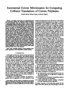
Fig. 1. Extremities of the arc A{1,3}

and the corresponding quadratic form (s0 , t0 ) ∈ R2 7→ q(s0 , t0 ) = [`(s0 , t0 )]2 . By working out formula (39), one gets p dist[x, K] = 1 − q(s, t), so our job consists in proving that 1 − q(s, t) ≤ (1 + α)/2.

(51)

Before taking care of (51), recall that the case J = {1} occurs exactly when (s, t) ∈ A{1} . From (48) , we know that A{1} = E+ \A{1,3} . This set is an arc of the ellipse E, closed at the extremity (s∗ , t∗ ), and open at the extremity (s0 , t0 ) = ([2(1 − α)]−1/2 , 0). We are supposing that γ − αβ > 0, because otherwise A{1} = ∅. Let us compute A{1} again, but this time using (37)–(38), that is to say, α(µ1 − s) + s − γt ≥ 0, β(µ1 − s) + γs − t ≥ 0. Plugging µ1 − s = tβ − sα into this system, we get after a short rearrangement (1 − α2 )s ≥ (γ − αβ)t, (γ − αβ)s ≥ (1 − β 2 )t. Since κ > 0, we have γ − αβ 1 − α2 < , 2 1−β γ − αβ

(52) (53)

Computing the Radius of Pointedness of a Convex Cone

17

and therefore (52) is redundant. In other words, the system (52)–(53) reduces to t ≤ ms. This confirms that the line Lm is cutting E+ into two disjoints arcs. We now proceed with the proof of (51). Observe that 1 − q(s, t) ≤ 1 − q(˜ s, t˜),

(54)

with (˜ s, t˜) being an arbitrary minimizer of q over the closed arc Ω = A{1} ∪ {(s0 , t0 )}. Since the linear form ` is positive over Ω, the point (˜ s, t˜) is also a minimizer of ` over Ω. Three different possibilities must be considered. If (˜ s, t˜) = (s0 , t0 ), then 1 − q(s, t) ≤ 1 − q(s0 , t0 ) = (1 + α)/2, and we are done. If (˜ s, t˜) = (s∗ , t∗ ), then we obtain (51) by using a continuity argument. Indeed, (s∗ , t∗ ) can be approached by a sequence {(sn , tn )}n∈N of points in A{1,3} . Projecting xn = sn (g1 − g2 ) + tn g3 into K produces a vector πK (xn ) lying in the relative interior of the face generated by g1 and g3 . As we have seen before, such a situation leads to the estimate {dist[xn , K]}2 ≤ (1 + α)/2. By passing to the limit, one gets 1 − q(s∗ , t∗ ) ≤ (1 + α)/2.

(55)

The inequality (51) follows then by combining (54) and (55). Finally, suppose that (˜ s, t˜) is not an extremity of the arc Ω. We claim that this case must be ruled out because it leads to a contradiction. Observe that now (˜ s, t˜) minimizes ` not only over Ω, but also over E. Recall that a non-zero linear form attains always a unique minimum over a non-degenerate ellipse. By inspecting the level sets of the linear form `, one sees that the value `(s, t) decreases when the argument (s, t) leaves the point (s0 , t0 ) and starts moving toward (˜ s, t˜) along the arc Ω. Since s and t are related through the relation (34), one can write p t(γ − β) + 2(1 − α) − t2 [2(1 − α) − (γ − β)2 ] (56) s = η(t) = 2(1 − α) for all t in some neighborhood V of t0 = 0. We are choosing, of course, the positive root of the quadratic equation (34). Define now ψ : V → R as p t(γ + β) + 2(1 − α) − t2 [2(1 − α) − (γ − β)2 ] . (57) ψ(t) = 2 It follows from (56) that `(η(t), t) = η(t)(1 − α) + tβ = ψ(t).

18

Alfredo Iusem, Alberto Seeger

From the previous discussion, we know that ψ(t) ≤ ψ(t0 ) for any t > 0 small enough, and therefore ψ 0 (t0 ) ≤ 0. But, on the other hand, a direct computation from (57) gives ψ 0 (t0 ) = (γ+β)/2. Since β+γ > 0 by (33), we get a contradiction. This confirms our claim and completes the proof of Lemma 6. t u Remark: The point (s∗ , t∗ ) has a special significance because it separates the regions corresponding to the cases J = {1} and J = {1, 3}. Actually, we did not use the formula that we got for (s∗ , t∗ ). It was enough to know that such a borderline point does exist.

5. The main result: proof and consequences The ground is now prepared for the proof of Theorem 1, our main result. Proof. Proposition 4 tells us that σ(K) ≤ ρ(K). Let L = R(u − v) be the line generated by u − v. By assumption, u and v are two unit vectors in K forming an angle equal to θmax (K). One can check that K ∩ L = {0}, so that K + L is a nonpointed closed convex cone. From the very definition of ρ(K), one has ρ(K) ≤ δ(K + L, K), so everything boils down to proving the inequality δ(K + L, K) ≤ σ(K).

(58)

Since K is a subset of K + L, we get from (2) δ(K + L, K) =

sup

dist[x, K],

x∈(K+L)∩SH

and, therefore, it is enough to show that dist[x, K] ≤ σ(K)

∀x ∈ (K + L) ∩ SH .

Suppose, on the contrary, that there exists x ˜ ∈ (K + L) ∩ SH such that dist[˜ x, K] > σ(K).

(59)

We decompose x ˜ in the form x ˜ = s(u − v) + ty,

with y ∈ K ∩ SH , s ∈ R, t ∈ R+ ,

and define C as the cone generated by g1 = u, g2 = v, and g3 = y. Observe that u, v are vectors in C ⊂ K achieving the maximal angle θmax (C) = θmax (K). Two cases must be distinguished: (i) Suppose first that the vectors {g1 , g2 , g3 } are linearly dependent. This implies that the linear space spanned by C is two-dimensional. This type of situation is well understood. In fact, it is not difficult to prove that σ(C) = ρ(C) = δ(C + L, C).

Computing the Radius of Pointedness of a Convex Cone

19

Since x ˜ ∈ (C +L)∩SH , one also has dist[˜ x, C] ≤ ρ(C). But dist[˜ x, K] ≤ dist[˜ x, C] and σ(C) = σ(K), so we are contradicting (59). (ii) Suppose now that the vectors {g1 , g2 , g3 } are linearly independent. By applying Lemma 6 to the cone C, we conclude that dist[˜ x, C] ≤ σ(C). As before, the inequalities dist[˜ x, K] ≤ dist[˜ x, C] and σ(C) = σ(K) lead to a contradiction with the assumption (59). t u The case of a perpendicular cone falls within the range of Theorem 1. Recall that a cone K ∈ Ξ(H) is said to be perpendicular if θmax (K) = π/2. This amounts to saying that K contains a pair of orthogonal unit vectors, and, in addition, hu, vi ≥ 0 ∀u, v ∈ K. √ Corollary 2. The radius of pointedness of any perpendicular cone is 2/2. Remark: Any self-dual cone is perpendicular. So, the Loewner cone √ of positive semidefinite symmetric matrices has a radius of pointedness equal to 2/2. The same remark applies to the Lorentz (or ice-cream) cone, and to the Pareto cone (or positive orthant). We recover in this way some particular results announced in [4].

6. By way of conclusion Theorem 1 has the merit of displaying a nice and simple formula for computing the radius of pointedness of a moderate cone K. The formula says that   θmax (K) . (60) ρ(K) = cos 2 In addition to this, Theorem 1 shows how to construct a nonpointed cone Q at minimal distance from K. A question that is bound to occur is the following one: is it possible to obtain the same conclusions as in Theorem 1, but without imposing the moderation assumption? As far as (60) is concerned, there are some facts suggesting that this formula may be true also for non-moderate cones. Consider, for instance, the case of a revolution cone K = {x ∈ H : kxkcos ϑ ≤ he, xi},

with e ∈ SH .

Even if we take θmax (K) = 2ϑ as large as we want, both sides of (60) yield the same value, namely cos ϑ. A more elaborate example is that of an elliptic cone p hx, Axi ≤ t}, K = {(x, t) ∈ Rd × R : with A being a positive semidefinite symmetric matrix of order d × d. Formula (60) turns out to be true for an arbitrary elliptic cone, be it moderate or not (see Theorem 8.3 in [4] for details).

20

Alfredo Iusem, Alberto Seeger

Although our proof method for Theorem 1 relies on the moderation assumption, there is some hope that formula (60) remains true over the whole Ξ(H). We show next that this is the case, if we manage to prove that ρ is antitone, meaning that ρ(K) ≥ ρ(K 0 ) whenever K ⊂ K 0 . Indeed, take an arbitrary K in Ξ(H). Let C ⊂ K be the 2-dimensonal cone generated by two unit vectors in K realizing its maximal angle. Under the antitonicity assumption, ρ(K) ≤ ρ(C). Since all 2-dimensional cones are revolution cones, we have ρ(C) = σ(C). Finally, the choice of C guarantees that C and K have the same maximal angle, so that σ(C) = σ(K). It follows that ρ(K) ≤ σ(K). The result is then a consequence of Proposition 4. However, one should not be over-optimistic either. As the next proposition shows, without the moderation assumption, at least one of the conclusions of Theorem 1 fails! Proposition 5. Let the dimension of H be at least three. For any angle θ ∈]2π/3, π[, there exist a cone K ∈ Ξ(H) and vectors u, v ∈ K ∩ SH such that (a) arccos hu, vi = θmax (K) = θ, (b) K + R(u − v) ∈ M(H), (c) δ(K + R(u − v), K) > σ(K). Proof. Take any θ ∈]2π/3, π[. We shall construct a non-moderate cone generated by three linearly independent unit vectors. Due to Proposition 3.2 of [4], there is no loss of generality in supposing that H = R3 . From the way the angle θ has been chosen, one sees that the coefficient p r = (1 + cos θ)/2 belongs to the interval ]0, 1/2[. Consider the cone K generated by the vectors  p  p  g1 = − 1 − r2 , r, 0 g2 = 1 − r2 , r, 0 , g3 =

p  p p p 1 2 2 , r 1 − 4r 2 , 4 − 12r 2 + 3 . 1 − r 1 − 4r 16r 2(1 − 2r2 )

This choice may seem quite strange at first sight, but, in fact, it is dictated by a certain number of requirements. To start with, observe that g1 and g2 are two unit vectors forming an angle equal to θ. Indeed, α = hg1 , g2 i = 2r2 − 1 = cos θ. Observe, incidentally, that α ∈ ] − 1, −1/2[. The first two components of g3 are chosen so that p − 2|α| − 1 , β = hg1 , g3 i = 2 p 2|α| − 1 γ = hg2 , g3 i = . 2|α|

Computing the Radius of Pointedness of a Convex Cone

21

Fig. 2. Non-moderate polyhedral cone generated by {g1 , g2 , g3 }

Finally, one chooses the last component of g3 so that kg3 k = 1. The vectors {g1 , g2 , g3 } are linearly independent, and one can easily check that β = αγ,

γ > αβ,

α < −1/2 < β < 0 < γ < 1.

Among the extreme rays {g1 , g2 , g3 } of the cone K, the pair (g1 , g2 ) forms the largest angle because α < β < γ. Although the maximal angle of a finitely generated cone may fail to be attained by a pair of extreme rays, this is not occurring in this particular example. Indeed, by using Theorem 6.4 of [5], it is possible to check that arccos hg1 , g2 i = θmax (K). (61) Take now  −1/2 s = 2(1 − α) − (γ − β)2 , t = (γ − β)s, x = s(g1 − g2 ) + tg3 . In such case, s > 0, t > 0, kxk = 1, and we are in the same setting as in the case J = {1, 3} of Lemma 6, that is to say, πK (x) belongs to the relative interior of the face of K generated by g1 and g3 . In view of (43)–(45), we can write kx − πK (x)k2 =

s2 [(1 − α2 )(1 − β 2 ) − (γ − αβ)2 ] . 1 − β2

If one replaces the value of s and subtracts [σ(K)]2 , one ends up with

1 − α2 1 − β 2 − (γ − αβ)2 1+α 2 2 kx − PK (x)k − [σ(K)] = − . (1 − β 2 ) [2(1 − α) − (γ − β)2 ] 2

22

Radius of Pointedness of a Convex Cone

Replacing β = αγ, we obtain, after some algebra, i
h 2 2 γ 2 1 − α2 −α − 12 − α 2γ kx − PK (x)k2 − [σ(K)]2 = . (1 − α2 γ 2 ) [2 − γ 2 (1 − α)] By expressing γ in terms of α, one gets finally
3(2α + 1)2 1 − α2 kx − PK (x)k − [σ(K)] = > 0. 2(5 + 2α)(6α2 + α + 1) 2

2

(62)

Thus, we have shown that kx − PK (x)k > σ(K). If we denote by L the line through g1 − g2 , then x ∈ (K + L) ∩ SH and δ(K + L, K) =

sup

dist[w, K] ≥ dist[x, K] = kx − PK (x)k.

w∈(K+L)∩SH

The conclusion is that δ(K + L, K) > σ(K).

t u

Observe that the expression on the right-hand side of (62) vanishes not only for α = −1/2, but also for α = −1. These values correspond, respectively, to θmax (K) = 2π/3 and θmax (K) = π. One can easily check that Theorem 1 is also true θmax (K) = π. So, it is the zone 2π/3 < θmax (K) < π that we view as a No Man’s Land where everything could happen. Acknowledgement. We are indebted to L.M. Gra˜ na Drummond (Federal University of Rio de Janeiro) for suggesting us the study of the coefficient σ. The comments provided by both referees were very helpful for improving the general presentation of this work.

References 1. Freund, R., Vera, J.R.: Condition-based complexity of convex optimization in conic linear form via the ellipsoid algorithm, SIAM Journal on Optimzation 10 (2000), 155-176. 2. Hiriart-Urruty, J.B.: Projection sur un cone convexe ferm´ e d’un espace euclidien. D´ ecomposition orthogonale de Moreau, Revue de Math´ ematiques Sp´ eciales (1989), 147-154. 3. Iusem, A., Seeger, A.: Pointedness, connectedness, and convergence results in the space of closed convex cones, Journal of Convex Analysis 11 (2004), 267-284. 4. Iusem, A., Seeger, A.: Measuring the degree of pointedness of a closed convex cone: a metric approach, Mathematische Nachrichten (2005), to appear. 5. Iusem, A., Seeger, A.: On pairs of vectors achieving the maximal angle of a convex cone, Mathematical Programming, (2005), to appear. 6. Iusem, A., Seeger, A.: Axiomatization of the index of pointedness of closed convex cones, Computational and Applied Mathematics, (2005), to appear. 7. Moreau, J.J.: D´ ecomposition orthogonale d’un espace hilbertien selon deux cones mutuellement polaires. Comptes Rendues de l’Acad´ emie des Sciences de Paris 255 (1962), 238-240. 8. Pe˜ na, J., Renegar, J.: Computing approximate solutions for conic systems of constraints, Mathematical Programming 87 (2000), 351-383. 9. Rockafellar, R.T., Wets, R.J.: Variational Analysis, Springer-Verlag, Berlin, 1998.