Apr 12, 2005 - ISSN 1458-9478. URL: http://cosco.hiit.fi/Articles/hiit-2005-1.pdf ..... In addition, this work was supported in part by the IST Programme of the Eu-.
COMPUTING THE REGRET TABLE FOR MULTINOMIAL DATA Petri Kontkanen, Petri Myllym¨aki
April 12, 2005
HIIT TECHNICAL REPORT 2005–1
COMPUTING THE REGRET TABLE FOR MULTINOMIAL DATA Petri Kontkanen, Petri Myllym¨aki
Helsinki Institute for Information Technology HIIT Tammasaarenkatu 3, Helsinki, Finland PO BOX 9800 FI-02015 TKK, Finland http://www.hiit.fi
HIIT Technical Reports 2005–1 ISSN 1458-9478 URL: http://cosco.hiit.fi/Articles/hiit-2005-1.pdf
c 2005 held by the authors Copyright °
NB. The HIIT Technical Reports series is intended for rapid dissemination of results produced by the HIIT researchers. Therefore, some of the results may also be later published as scientific articles elsewhere.
Computing the Regret Table for Multinomial Data Petri Kontkanen, Petri Myllym¨aki Complex Systems Computation Group (CoSCo) Helsinki Institute for Information Technology (HIIT) University of Helsinki & Helsinki University of Technology P.O. Box 9800, FIN-02015 HUT, Finland. {Firstname}.{Lastname}@hiit.fi Abstract Stochastic complexity of a data set is defined as the shortest possible code length for the data obtainable by using some fixed set of models. This measure is of great theoretical and practical importance as a tool for tasks such as model selection or data clustering. In the case of multinomial data, computing the modern version of stochastic complexity, defined as the Normalized Maximum Likelihood (NML) criterion, requires computing a sum with an exponential number of terms. Furthermore, in order to apply NML in practice, one often needs to compute a whole table of these exponential sums. In our previous work, we were able to compute this table by a recursive algorithm. The purpose of this paper is to significantly improve the time complexity of this algorithm. The techniques used here are based on the discrete Fourier transform and the convolution theorem.
1
Introduction
The Minimum Description Length (MDL) principle developed by Rissanen [Rissanen, 1978; 1987; 1996] offers a wellfounded theoretical formalization of statistical modeling. The main idea of this principle is to represent a set of models (model class) by a single model imitating the behaviour of any model in the class. Such representative models are called universal. The universal model itself does not have to belong to the model class as often is the case. From a computer science viewpoint, the fundamental idea of the MDL principle is compression of data. That is, given some sample data, the task is to find a description or code of the data such that this description uses less symbols than it takes to describe the data literally. Intuitively speaking, this approach can in principle be argued to produce the best possible model of the problem domain, since in order to be able to produce the most efficient coding of data, one must capture all the regularities present in the domain. The MDL principle has gone through several evolutionary steps during the last two decades. For example, the early realization of the MDL principle, the two-part code MDL [Rissanen, 1978], takes the same form as the Bayesian BIC criterion [Schwarz, 1978], which has led some people to incor-
rectly believe that MDL and BIC are equivalent. The latest instantiation of the MDL is not directly related to BIC, but to the formalization described in [Rissanen, 1996]. Unlike Bayesian and many other approaches, the modern MDL principle does not assume that the chosen model class is correct. It even says that there is no such thing as a true model or model class, as acknowledged by many practitioners. The model class is only used as a technical device for constructing an efficient code. For discussions on the theoretical motivations behind the modern definition of the MDL see, e.g., [Rissanen, 1996; Merhav and Feder, 1998; Barron et al., 1998; Gr¨unwald, 1998; Rissanen, 1999; Xie and Barron, 2000; Rissanen, 2001]. The most important notion of the MDL principle is the Stochastic Complexity (SC), which is defined as the shortest description length of a given data relative to a model class M. However, the applications of the modern, so called Normalized Maximum Likelihood (NML) version of SC, at least with multinomial data, have been quite rare. The modern definition of SC is based on the Normalized Maximum Likelihood (NML) code [Shtarkov, 1987]. Unfortunately, with multinomial data this code involves a sum over all the possible data matrices of certain length. Computing this sum, usually called the regret, is obviously exponential. Therefore, practical applications of the NML have been quite rare, In our previous work [Kontkanen et al., 2003; 2005], we presented a polynomial time (quadratic) method to compute the regret. In this paper we improve our previous results and show how mathematical techniques such as discrete Fourier transform and fast convolution can be used in regret computation. The idea of applying these techniques to the regret computation problem was first suggested in [Koivisto, 2004], but as discussed in [Kontkanen et al., 2005], in order to apply NML to practical tasks such as clustering, a whole table of regret terms is needed. We will modify the method of [Koivisto, 2004] for this task. In Section 2 we shortly review how the stochastic complexity is defined and our previous work on the computational methods. We also introduce the concept of the regret table. Section 3 previews some mathematical results about convolution and discrete Fourier transform and presents the new fast convolution-based NML algorithm. Finally, Section 4 gives the concluding remarks and presents some ideas for future work.
2
Stochastic Complexity for Multinomial Data
2.1 NML And Stochastic Complexity The most important notion of the MDL is the Stochastic Complexity (SC). Intuitively, stochastic complexity is defined as the shortest description length of a given data relative to a model class. To formalize things, let us start with a definition of a model class. Consider a set Θ ∈ Rd , where d is a positive integer. A class of parametric distributions indexed by the elements of Θ is called a model class. That is, a model class M is defined as M = {P (· | θ) : θ ∈ Θ}.
(1) N
Consider now a discrete data set (or matrix) x = (x1 , . . . , xN ) of N outcomes, where each outcome xj is an element of the set X consisting of all the vectors of the form (a1 , . . . , am ), where each variable (or attribute) ai takes ˆ N ) denote on values v ∈ {1, . . . , ni }. Furthermore, let θ(x the maximum likelihood estimate of data xN , i.e., ˆ N ) = arg max{P (xN | θ)}. θ(x
(2)
θ∈Θ
The Normalized Maximum Likelihood (NML) distribution [Shtarkov, 1987] is now defined as PN M L (xN | M) =
ˆ N ), M) P (xN | θ(x , RN M
where RN M is given by X ˆ N ), M), RN P (xN | θ(x M =
(3)
(4)
xN
and the sum goes over all the possible data matrices of size N . The term RN M is called the regret. The definition (3) is intuitively very appealing: every data matrix is modeled using its own maximum likelihood (i.e., best fit) model, and then a penalty for the complexity of the model class M is added to normalize the distribution. The stochastic complexity of a data set xN with respect to a model class M can now be defined as the negative logarithm of (3), i.e., ˆ N ), M) P (xN | θ(x (5) RN M ˆ N ), M) + log RN . (6) = − log P (xN | θ(x M
SC(xn | M) = − log
2.2 NML for Single Multinomial Model Class In this section we instantiate the NML distribution (3) (and thus the stochastic complexity) for the single-dimensional multinomial case. Let us assume that a discrete random variable X with K values is multinomially distributed. That is, the parameter set Θ is a simplex Θ = {(θ1 , . . . , θK ) : θk ≥ 0, θ1 + · · · + θK = 1},
(7)
where θk = P (X = k), k = 1, . . . , K.
(8)
We denote this model class by MK . Now consider a data sample of size N from the distribution of X, i.e., xN = (x1 , . . . , xN ) and each xj ∈ {1, . . . , K}. The likelihood is clearly given by K N N Y Y Y (9) θkhk , θxj = P (xj | θ) = P (xN | θ) = j=1
j=1
k=1
where hk is the frequency of value k in xN . Numbers (h1 , . . . , hK ) are called the sufficient statistics of data xN . Word “sufficient” refers to the fact that the likelihood depends on the data only through them. To instantiate the NML distribution (3) for the MK model class, we need to find the maximum likelihood estimates for the parameters θk . As one might intuitively guess, the ML parameters are given by the relative frequencies of the values k in the data (see, e.g., [Johnson et al., 1997]): ˆ N ) = (θˆ1 , . . . , θˆK ) θ(x (10)
h1 hK ,..., ). (11) N N Thus, the likelihood evaluated at the maximum likelihood point is ¶h K µ Y hk k N ˆ N , (12) P (x | θ(x )) = N =(
k=1
and the NML distribution becomes QK ¡ hk ¢hk N , PN M L (x | MK ) = k=1N N RMK where X ˆ N ), MK ) RN P (xN | θ(x MK =
(13)
(14)
xN
=
X
h1 +···+hK =N
¶h K µ Y hk k N! , h1 ! · · · hK ! N
(15)
k=1
and the sum goes over all the compositions of N into K parts, i.e., over all the possible ways to choose a vector of nonnegative integers (h1 , . . . , hK ) such that they sum up to N . The N !/(h1 ! · · · hK !) factor in (15) is called the multinomial coefficient and it is one of the basic combinatorial quantities. It counts the number of arrangements of N objects into K boxes each containing h1 , . . . , hK objects, respectively. An efficient method for computing (15) was derived in [Kontkanen et al., 2003]. It is based on the following recursive formula: ¶h K µ X Y N! hk k N RMK = (16) h1 ! · · · hK ! N h1 +···+hK =N k=1 X N ! ³ r1 ´r1 ³ r2 ´r2 1 2 · RrM · RrM = k1 k2 r1 !r2 ! N N r1 +r2 =N
(17)
N ³ r ´r µ N − r ¶N −r X N! = r!(N − r)! N N r=0
−r (18) · RrMk1 · RN Mk2 , where k1 + k2 = K. See [Kontkanen et al., 2003] for details.
n/k 0 1 ··· N
2.3 NML for Clustering Model Class In [Kontkanen et al., 2005] we discussed NML computation methods for a multi-dimensional model class suitable for cluster analysis. The selected model class has also been successfully applied to mixture modeling [Kontkanen et al., 1996], case-based reasoning [Kontkanen et al., 1998], Naive Bayes classification [Gr¨unwald et al., 1998; Kontkanen et al., 2000b] and data visualization [Kontkanen et al., 2000a].
1 R01 R11 ··· RN 1
2 R02 R12 ··· RN 2
case: X
RN MT ,K =
h1 +···+hK =N
·
K m Y Y
= P (ai | c, MT ).
(19) Suppose the special variable c has K values and each ai has ni values. The NML distribution for the model class MT is now
PN M L (xN | MT ) =
¶f ¶h m K ni µ K µ Y hk k Y Y Y fikv ikv
k=1
·
N
i=1 k=1 v=1
1
RN MT ,K
hk
,
(20)
where hk is the number of times c has value k in xN , fikv is the number of times ai has value v when c = k, and RN MT ,K is the regret
X
RN MT ,K =
h1 +···+hK =N
·
K m Y Y
¶h K µ Y hk k N! h1 ! · · · hK ! N k=1
X
i=1 k=1 fik1 +···+fikni =hk
·
¶f ni µ Y fikv ikv
v=1
h1 +···+hK =N
·
(21)
hk
X
=
hk ! fik1 ! · · · fikni !
m Y K Y
i=1 k=1
¶h K µ Y hk k N! h1 ! · · · hK ! N k=1
RhMk n . i
(22)
It turns out [Kontkanen et al., 2005] that the recursive formula (18) can be generalized also to this multi-dimensional
k=1
(23)
i
N ! ³ r1 ´r1 ³ r2 ´r2 r1 !r2 ! N N
r1 +r2 =N 1 · RrM T ,k1
i=1
"
X
¶h K µ Y n! hk k h1 ! · · · hK ! N
RhMk n
i=1 k=1
P (c, a1 , . . . , am | MT ) = P (c | MT )
K R0K R1K ··· RN K
Table 1: The regret table.
Let us assume that we have m variables, (a1 , . . . , am ). We also assume the existence of a special variable c (which can be chosen to be one of the variables in our data or it can be latent) and that given the value of c, the variables (a1 , . . . , am ) are independent. The resulting model class is denoted by MT . Our assumptions can now be written as m Y
··· ··· ··· ··· ···
2 · RrM T ,k2
(24)
N ³ r ´r µ N − r ¶N −r X N! = r!(N − r)! N N r=0 −r · ·RrMT ,k1 · RN MT ,k2 ,
#
(25)
where k1 + k2 = K.
2.4 The Regret Table As discussed in [Kontkanen et al., 2005], in order to apply NML to the clustering problem, two tables of regret terms are needed. The first one consists of the one-dimensional terms RnMk for n = 0, . . . , N and k = 1, . . . , n∗ , where n∗ is defined by n∗ = max{n1 , . . . , nm }. The second one holds the multi-dimensional regret terms needed in computing the stochastic complexity PN M L (xN | MT ). More precisely, this table consists of the terms RnMT ,k for n = 0, . . . , N and k = 1, . . . , K, where K is the maximum number of clusters. The idea of the regret table can also be generalized. The natural candidate for the first dimension of the table is the size of the data. In addition to number of values or clusters, the other dimension can be, e.g., number of classes in classification tasks, or number of components in mixture modeling. The regret table is figured in Table 1. For the single-dimensional multinomial case, the procedure of computing the regret table starts by filling the first column, i.e., the case k = 1. This is trivial, since clearly RnM1 = 1 for all n = 0, . . . , N . To compute the column k, for k = 2, . . . , K, the recursive formula (18) can be used by choosing, e.g., k1 = k − 1,¡ k2 = 1.¢ The time complexity of filling the whole table is O K · N 2 . The multi-dimensional case is very similar, since the recursion formula is essentially the same. The only exception is the computation of the first column. When k = 1, Equation (22) reduces to m Y (26) RnMn , RnMT ,1 = i
i=1
for n = 0, . . . , N . After these easy calculations, the rest of the regret table can be filled by applying the recursion (25) similarly as in the single-dimensional case. The time complexity ¡of calculating the multi-dimensional regret table is ¢ also O K · N 2 . In practice, the quadratic dependency on the size of data in both the single- and multi-dimensional cases limits the applicability of NML to small or moderate size data sets. In the next section, we will present a novel, significantly more efficient method for computing the regret table.
3
3.1 Discrete Fourier Transform Consider a finite-length sequence of real or complex numbers a = (a0 , a1 , . . . , aN −1 ). The Discrete Fourier Transform (DFT) of a is defined as a new sequence A with ah · e2πihn/N
(27)
µ ¶ 2πhn 2πhn ah · cos + i sin , N N
(28)
h=0
=
N −1 X h=0
for n = 0, . . . , N − 1. A very intuitive explanation of the DFT is presented in [Wilf, 2002], where it is shown that if the original sequence is interpreted as the coefficients of a polynomial, the Fourier transformed sequence is obtained by evaluating the values of this polynomial at certain points on the complex unit circle. See [Wilf, 2002] for details. To recover the original sequence a given the transformed sequence A, the Discrete inverse Fourier Transform (DFT−1 ) is used. The definition of DFT−1 is very similar to DFT, and it is given by N −1 1 X Ah · e−2πihn/N N h=0 ¶ µ N −1 2πhn 1 X 2πhn − i sin , = Ah · cos N N N
an =
where
n X
ah bn−h , n = 0, . . . , N − 1.
(31) (32)
(33)
h=0
As mentioned in [Koivisto, 2004], the so-called fast convolution algorithm can be used to derive very efficient methods for regret computation. In this section, we will present a version suitable for computing regret tables. We will start with some mathematical background, and then proceed by deriving the fast NML algorithm.
An =
c=a∗b = (c0 , c1 , . . . , cN −1 ),
cn =
Fast Convolution
N −1 X
section, we will briefly review basic properties of convolution that are relevant to the discussion of the rest of the section. Let a = (a0 , a1 , . . . , aN −1 ) and b = (b0 , b1 , . . . , bN −1 ) be two sequences of length N . The convolution of a and b is defined as a sequence c,
(29)
(30)
h=0
for n = 0, . . . , N − 1. A trivial algorithm for computing ¡the ¢discrete Fourier transform of length N takes time O N 2 . However, by means of the classic Fast Fourier Transform (FFT) algorithm (see, e.g., [Wilf, 2002]), this can be improved to O (N log N ). As we will soon see, the FFT algorithm is the basis of the fast regret table computation method.
3.2 The Convolution Theorem A mathematical concept of convolution turns out to be a key element in the derivation of the fast NML algorithm. In this
Note that the convolution is mathematically equivalent to polynomial multiplication if the contents of the sequences are interpreted as the coefficients of the polynomials. A direct of the convolution (33) clearly takes ¡ computation ¢ time O N 2 . The convolution theorem shows how to compute convolution via the discrete Fourier transform: Let a = (a0 , a1 , . . . , aN −1 ) and b = (b0 , b1 , . . . , bN −1 ) be two sequences. The convolution of a and b can be computed as c = a ∗ b = DFT−1 (DFT(a) · DFT(b)),
(34)
where all the vectors are zero padded to length 2N , and the multiplication is component-wise. In other words, the Fourier transform of the convolution of two sequences is equal to the product of the transforms of the individual sequences. Since both the DFT and DFT−1 can be computed in time O (N log N ) via the FFT algorithm, and the multiplication in (34) only takes time O (N ), it follows that the time complexity of computing the convolution sequence via DFT is O (N log N ).
3.3 The Fast NML Algorithm In this section we will show how the fast convolution algorithm can be used to derive a very efficient method for the regret table computation. The new method replaces the recursion formulas (18) and (25) discussed in the previous section. Our goal here is to calculate the column k of the regret table given the first k − 1 columns. Let us define two sequences a and b by nn n nn n Rk−1 , bn = R . (35) an = n! n! 1 Evaluate now the convolution of a and b, n X hh h (n − h)n−h n−h R R1 (36) h! k−1 (n − h)! h=0 µ ¶h µ ¶n−h n nn X n! h n−h = n! h!(n − h)! n n
(a ∗ b)n =
h=0
· Rhk−1 R1n−h
(37)
n
=
n Rn , n! k
(38)
where the last equality follows from the recursion formulas (18) and (25). This derivation shows that the column k can be computed by first evaluating the convolution (38), and then multiplying each term by n!/nn .
It is now clear that by computing the convolutions via the DFT method discussed in the previous section, the time complexity of computing the whole regret table drops to ¡O (N log ¢ N · K). This is a major improvement over O N 2 · K obtained by the recursion method of Section 2.
4
Conclusion And Future Work
In this paper we discussed efficient computation algorithms for normalized maximum likelihood computation in the case of multinomial data. The focus was on the computation of the regret table needed by many applications. We showed how advanced mathematical techniques such as discrete Fourier transform and convolution can be applied to the problem. The main result of the paper is a derivation of a novel algorithm for regret table computation. The theoretical time complexity of this algorithm allows practical applications of NML in domains with very large datasets. With the earlier quadratic-time algorithms, this was not possible. In the future, we plan to conduct an extensive set of empirical tests to see how well the theoretical advantage of the new algorithm transfers to practice. On the theoretical side, our goal is to extend the regret table computation to more complex cases like general graphical models. We will also research supervised versions of the stochastic complexity, designed for supervised prediction tasks such as classification. Acknowledgements This work was supported in part by the Academy of Finland under the projects Minos and Civi and by the National Technology Agency under the PMMA project. In addition, this work was supported in part by the IST Programme of the European Community, under the PASCAL Network of Excellence, IST-2002-506778. This publication only reflects the authors’ views.
References [Barron et al., 1998] A. Barron, J. Rissanen, and B. Yu. The minimum description principle in coding and modeling. IEEE Transactions on Information Theory, 44(6):2743– 2760, October 1998. [Gr¨unwald et al., 1998] P. Gr¨unwald, P. Kontkanen, P. Myllym¨aki, T. Silander, and H. Tirri. Minimum encoding approaches for predictive modeling. In G. Cooper and S. Moral, editors, Proceedings of the 14th International Conference on Uncertainty in Artificial Intelligence (UAI’98), pages 183–192, Madison, WI, July 1998. Morgan Kaufmann Publishers, San Francisco, CA. [Gr¨unwald, 1998] P. Gr¨unwald. The Minimum Description Length Principle and Reasoning under Uncertainty. PhD thesis, CWI, ILLC Dissertation Series 1998-03, 1998. [Johnson et al., 1997] N.L. Johnson, S. Kotz, and N. Balakrishnan. Discrete Multivariate Distributions. John Wiley & Sons, 1997. [Koivisto, 2004] M. Koivisto. Sum-Product Algorithms for the Analysis of Genetic Risks. PhD thesis, Report A2004-1, Department of Computer Science, University of Helsinki, 2004.
[Kontkanen et al., 1996] P. Kontkanen, P. Myllym¨aki, and H. Tirri. Constructing Bayesian finite mixture models by the EM algorithm. Technical Report NC-TR-97-003, ESPRIT Working Group on Neural and Computational Learning (NeuroCOLT), 1996. [Kontkanen et al., 1998] P. Kontkanen, P. Myllym¨aki, T. Silander, and H. Tirri. On Bayesian case matching. In B. Smyth and P. Cunningham, editors, Advances in CaseBased Reasoning, Proceedings of the 4th European Workshop (EWCBR-98), volume 1488 of Lecture Notes in Artificial Intelligence, pages 13–24. Springer-Verlag, 1998. [Kontkanen et al., 2000a] P. Kontkanen, J. Lahtinen, P. Myllym¨aki, T. Silander, and H. Tirri. Supervised model-based visualization of high-dimensional data. Intelligent Data Analysis, 4:213–227, 2000. [Kontkanen et al., 2000b] P. Kontkanen, P. Myllym¨aki, T. Silander, H. Tirri, and P. Gr¨unwald. On predictive distributions and Bayesian networks. Statistics and Computing, 10:39–54, 2000. [Kontkanen et al., 2003] P. Kontkanen, W. Buntine, P. Myllym¨aki, J. Rissanen, and H. Tirri. Efficient computation of stochastic complexity. In C. Bishop and B. Frey, editors, Proceedings of the Ninth International Conference on Artificial Intelligence and Statistics, pages 233–238. Society for Artificial Intelligence and Statistics, 2003. [Kontkanen et al., 2005] P. Kontkanen, P. Myllym¨aki, W. Buntine, J. Rissanen, and H. Tirri. An MDL framework for data clustering. In P. Gr¨unwald, I.J. Myung, and M. Pitt, editors, Advances in Minimum Description Length: Theory and Applications. The MIT Press, 2005. [Merhav and Feder, 1998] N. Merhav and M. Feder. Universal prediction. IEEE Transactions on Information Theory, 44(6):2124–2147, October 1998. [Rissanen, 1978] J. Rissanen. Modeling by shortest data description. Automatica, 14:445–471, 1978. [Rissanen, 1987] J. Rissanen. Stochastic complexity. Journal of the Royal Statistical Society, 49(3):223–239 and 252–265, 1987. [Rissanen, 1996] J. Rissanen. Fisher information and stochastic complexity. IEEE Transactions on Information Theory, 42(1):40–47, January 1996. [Rissanen, 1999] J. Rissanen. Hypothesis selection and testing by the MDL principle. Computer Journal, 42(4):260– 269, 1999. [Rissanen, 2001] J. Rissanen. Strong optimality of the normalized ML models as universal codes and information in data. IEEE Transactions on Information Theory, 47(5):1712–1717, July 2001. [Schwarz, 1978] G. Schwarz. Estimating the dimension of a model. Annals of Statistics, 6:461–464, 1978. [Shtarkov, 1987] Yu M. Shtarkov. Universal sequential coding of single messages. Problems of Information Transmission, 23:3–17, 1987.
[Wilf, 2002] H. S. Wilf. Algorithms and Complexity. A K Peters, Ltd., 2002. [Xie and Barron, 2000] Q. Xie and A.R. Barron. Asymptotic minimax regret for data compression, gambling, and prediction. IEEE Transactions on Information Theory, 46(2):431–445, March 2000.