Establishing high-level relationships between the flow physics governing SRP and design choices related to vehicle configuration and system performance will ...
CONCEPTUAL MODELING OF SUPERSONIC RETROPROPULSION FLOW INTERACTIONS AND THE RELATIONSHIP TO SYSTEM PERFORMANCE Ashley M. Korzun and Robert D. Braun Georgia Institute of Technology, Atlanta, Georgia, USA
ABSTRACT
in support of numerous design trades may be infeasible with current computational capabilities.
Supersonic retropropulsion is an entry, descent, and landing technology applicable to and potentially enabling the high-mass missions to the surface required for advanced robotic and human exploration at Mars. For conceptual design, an initial understanding of the significance of retropropulsion configuration on the vehicle’s static aerodynamic characteristics and the relation of this configuration to other vehicle performance metrics that traditionally determine vehicle configuration is necessary. This work develops an approximate model for the aerodynamic - propulsive flow interaction based on momentum transfer within the flowfield and the geometry of relevant flow structures. This model is used to explore the impact of operating conditions, required propulsion system performance, propulsion system composition, and vehicle configuration on the integrated aerodynamic drag characteristics of full-scale vehicles for Mars entry, descent, and landing. Conclusions are then drawn on the fidelity and effort required to support specific design trades for supersonic retropropulsion.
In place of high-fidelity aerodynamic analyses, an approximate model for the SRP aerodynamic - propulsive interaction can be used to provide an initial understanding of the significance of SRP configuration on the vehicle’s aerodynamic characteristics. These effects can then be related to other performance metrics traditionally determining vehicle configuration. Establishing high-level relationships between the flow physics governing SRP and design choices related to vehicle configuration and system performance will also assist in determining the fidelity and effort required to evaluate individual SRP concepts.
Key words: Mars exploration; entry, descent, and landing (EDL); supersonic retropropulsion (SRP).
1.
INTRODUCTION
Supersonic deceleration has been identified as a critical deficiency in extending heritage technologies to the highmass systems required to achieve long-term exploration goals at Mars. Supersonic retropropulsion (SRP), or the use of retropropulsive thrust while an entry vehicle is traveling at supersonic conditions, is a technology potentially amending this deficiency. SRP aerodynamic propulsive interactions alter the aerodynamic characteristics of the vehicle, and models must be developed that accurately represent the impact of SRP on system mass and performance. While systems analyses will rely heavily on high-fidelity computational methods to develop these models, existing computational tools and approaches applied to SRP flow interactions are computationally expensive in accurately and consistently simulating the features and behaviors of SRP flowfields. Use of such approaches
Experimental efforts have determined that flowfield structure and flowfield stability for SRP are highly dependent on the retropropulsion configuration, the strength of the retropropulsion exhaust flow relative to the strength of the freestream flow, and the expansion condition of the jet flow. Momentum transfer within the flowfield governs the change in the surface pressure distribution of the vehicle, and accordingly, governs the change in the vehicle’s integrated static aerodynamic characteristics. Parameters governing SRP aerodynamics have been identified using both experimental trends from the literature and analytical relations of momentum transfer within the SRP flowfield. These analytical relations are specific to highly under-expanded jet flows, contact surfaces, and blunt bodies in supersonic flows. In this study, a momentum-based, analytical flow model is developed and then used to explore the impact of SRP operating conditions, required propulsion system performance, propulsion system composition, and vehicle configuration on the integrated aerodynamic drag characteristics of full-scale vehicles for Mars entry, descent, and landing (EDL). This is completed through assessment of relative changes in surface pressure, integrated aerodynamic drag coefficient, and total axial force coefficient as functions of the maximum vehicle thrust-to-weight ratio (T /W ), the number of nozzles amongst which the thrust is distributed, and jet flow composition. Relative differences in these quantities and physical changes in flowfield structure are used to identify the fidelity and effort required to support specific design trades for SRP.
2.
APPROACH
The computational expense of using high-fidelity tools to simulate SRP flowfields prohibits using such tools for high-level trade studies. Development of an approximate model for the SRP aerodynamic - propulsive interaction provides an approach for understanding the relative significance of different design choices. This section discusses the general approach taken to evaluate the sensitivity of aerodynamic drag and total axial force to systemlevel design choices. Development of the flowfield model used to obtain these quantities is discussed in detail in Section 3. Design choices to be faced by mission planners include SRP operating conditions (e.g. freestream conditions), the required propulsion system performance (e.g. Isp , (T /W )max ), propulsion system type (e.g. propellant combination, j ), nozzle geometry (e.g. Ae /A⇤ and potential system packaging impacts), and vehicle configuration (e.g. the number of nozzles distributing thrust). While each of these design choices is related to the others, an effort has been made here to establish a parametric approach to illustrate the significance of specific design choices. Three different physical scales are used to distinguish the effects of SRP and to identify differences arising from vehicle scale and application. These are a human-scale SRP system for a vehicle at Mars, a roboticscale SRP system for a precursor or technology demonstration mission at Mars, and a sub-scale, cold-gas model for experimentation in a wind tunnel or other Earth-based ground test facility. The operational envelope for SRP has been defined through analysis determining the optimal trajectories that minimize propulsion system mass (see [1]). The propulsion system performance required to achieve these trajectories is a strong function of the constraints on the analysis. For example, constraining the vehicle (T /W )max to minimize propulsion system mass and volume results in a vehicle (T /W )max approximately three times smaller than constraining the vehicle to a maximum sensed acceleration of 4 (Earth) g’s. The smaller (T /W )max results in lower thrust levels and operation at higher freestream Mach numbers. Vehicle (T /W )max is used here as a parameter to represent the operational SRP envelope for a human-scale vehicle, ranging from 3.5 to 10.0 (Marsrelative). This range spans the values of (T /W )max determined in [1] and those used in NASA EDL-SA work [2]. Baseline vehicle concepts utilize multiple nozzle propulsion systems to improve system reliability, to provide redundancy, and to allow for greater control authority during powered descent [2]. The results of [3–5] demonstrated that there can be flowfield differences between a single nozzle and multiple nozzles providing the same total thrust. With the dependence of the SRP aerodynamic - propulsive interaction on the relative areas of the nozzle exit and vehicle forebody and the desire to use multiple nozzles on a flight vehicle, the number of nozzles is a de-
sign choice. The configuration of multiple nozzles is assumed to consist of equally-spaced nozzles arranged in a ring and aligned parallel with and opposite the freestream flow direction. The change in the vehicle’s static aerodynamic performance is explored for cases with the required thrust distributed over 3, 4, 5, and 6 nozzles for a human-scale SRP system. The effect of varying the number of nozzles is also examined for a robotic precursor/technology demonstrator mission. A full-scale LOX/CH4 propulsion system capable of satisfying the thrust and throttling requirements defined in NASA mission concepts does not currently exist. However, propulsion system mass and volume for the same V requirement have been shown to be comparable between theoretical LOX/CH4 systems and existing LOX/RP-1 systems [1]. The differences in SRP flowfield structure are explored for variations in the composition of the exhaust gas. Exhaust gas characteristics representative of different propellant types (LOX/CH4 , LOX/RP1, and LOX/LH2 ) are considered for both full-scale and sub-scale applications. The emphasis is on changes in the aerodynamic properties of the nozzle flow that would arise as propulsion system types are traded. 3.
FLOWFIELD MODEL DEVELOPMENT
This section describes the development of an approximate model for the SRP aerodynamic - propulsive interaction. The flow model is derived from a momentum - force balance at the contact surface and the geometry of the jet flow, body, and contact surface. All assumptions about the structure of the SRP flowfield are consistent with the discussion presented in [3, 6]. Elements of the flow model leverage analytical work in the literature. The flow model structure is directly based on analytical and experimental work by Finley [6] from the mid1960s. Finley’s model is strictly limited to hemispherical bodies, sonic nozzles (Me = 1), air as the composition of the freestream and jet flows ( 1 = j = 1.4), a single, central nozzle, and small jet structures relative to the diameter of the body. In this section, Finley’s original model is re-derived to generalize the flow model to Me > 1, j and 1 other than 1.4, forebody shapes other than hemispheres, and multiple nozzles on the forebody. These modifications extend the applicability of the flow model to the conditions and geometries more relevant to SRP system design. 3.1.
Overview of Aerodynamic - Propulsive Interaction Model
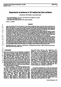
Fig. 1 illustrates the structure and progression of steps for the SRP flow model. Inputs to the model are the freestream conditions (M1 , 1 , p0,1 , T0,1 ), nozzle conditions ( j , p0,j , T0,j ), nozzle geometry (Ae /A⇤ or de ), and body geometry (dbody , rn ). Outputs from the model are the surface pressure (excluding the nozzle exit
plane), forebody integrated drag coefficient, and forebody axial force coefficient. There are two main elements to the SRP flow model. The first is a control surface analysis for the momentum - force balance at the contact surface (subscript: cs, M F ). The second is an analysis based on the flowfield geometry to match the contact surface to the body (subscript: cs, F G). Freestream conditions, nozzle conditions, nozzle geometry, body geometry, guess for α"
Inputs / Outputs"
α" Momentum – Force Balance 1. Integration of pressures on control surface to obtain force 2. Summation of jet flow entering and flow in jet layer leaving to obtain total momentum flux out of control surface 3. Equation of momentum flux out of control surface and forces on control surface to solve for dcs,M-F"
Flowfield Geometry Analysis 1. Finite-difference approach for isentropic free jet expansion (Mach disk location and diameter) 2. Continuity relation in stagnation region (contact surface location relative to nozzle exit) 3. Similar triangles relations to match the contact surface to the body and to solve for dcs,FG"
dcs,FG"
dcs,M-F"
Iterate on α until dcs,M-F = dcs,FG"
Dead-air Region Pressure
pda = p0,2 − ( p0,2 − p∞ )cos2 α Integration of Forebody Pressure Distribution
CD,f and CA,f"
€
CA, f = CD, f + CT
€
Figure 1. General structure of the flow model.
Integration of pressures over the control surface yields the force on the control surface. The summation of the jet flow entering the control surface and the flow in the jet layer exiting the control surface yields the total momentum flux out of the control surface. The diameter of the contact surface, dcs,M F , is then determined from the momentum - force balance. The definition of the control surface and additional details and discussion on this element of the flow model are given in Section 3.2. The flowfield geometry analysis establishes the diameter and axial location of the contact surface from the physics and structure of the jet interaction region. The Mach disk location and diameter are provided by an analytical finitedifference approach developed by Salas [7]. A continuity relation is applied in the stagnation region to determine the location of the contact surface, relative to the nozzle exit. Similar triangles are then used to match the contact surface to the body, yielding the diameter of the contact surface, dcs,F G . Additional details and discussion on the flowfield geometry analysis are given in Section 3.3. There are two independent variables in the analysis: P and ↵. P is specified by the conditions of interest, namely
the total pressure of the jet and the freestream conditions (P = p0,j /p0,2 ). The half-angle of the cone partially defining the shape of the contact surface is defined to be the angle ↵ that permits the diameter of the blunting sphere of the contact surface (determined from conservation of momentum within the flowfield) to be equal to the diameter of the blunting sphere of the contact surface determined from the structure of the jet. The model iterates on ↵ until dcs,M F matches dcs,F G . The pressure distribution on the contact surface is then determined as a function of ↵ and the pressure in the recirculation region by assuming modified-Newtonian theory. To determine the surface pressure distribution on the body, the pressure in the recirculating region is assumed to be a uniform pressure acting over the entire forebody surface outboard of the nozzle(s) with the exception of the nozzle exit area(s). Following Finley’s original notation, this pressure is referred to as the ‘dead-air’ pressure, pda , and is calculated using the equation shown in Fig. 1. Experimental investigations have observed surface pressures to decrease rapidly to near-constant values outside of the nozzle and over much of the forebody for moderate to high jet pressure ratios (see [4, 5, 8]). In this analysis, the pressure distribution across the forebody is assumed to be constant; no model for pressure recovery toward the shoulder has been implemented in this work. The forebody drag coefficient, CD,f is then calculated by integrating the surface pressure distribution, excluding the nozzle exit area(s). With all cases defined to be at zero angle of attack, the total axial force coefficient, CA,f , is then determined as the sum of CD,f and CT . The thrust coefficient, CT , is a force coefficient, defined in Eq. 1, where T is the thrust, q1 is the freestream dynamic pressure, and Aref is the aerodynamic reference area.
CT =
T q1 Aref
(1)
The flow model has been verified against analytical results from Finley [6] and validated against experimental results from multiple sources, including a recent NASA wind tunnel test [6, 8, 9]. In the development of the model, the flow is assumed to be steady, inviscid, isentropic, and behave as a calorically perfect gas. The flowfield is assumed to be axisymmetric. Sections 3.2 - 3.4 discuss the flow model in detail, including the historical references on which portions of the analysis are based, the modifications made to Finley’s original flow model, and the solution process for the surface pressure and integrated aerodynamic drag and total axial force coefficients for the forebody. 3.2.
Momentum - Force Balance Analysis
The first portion of the overall flowfield analysis is a momentum - force balance at the contact surface. Fig. 2
shows the general characteristics of an SRP flowfield with a single nozzle at the center of a blunt body, indicating the locations of the bow shock, contact surface, and Mach disk. Adapted from Finley [6], Fig. 3 shows the control surface (dashed line and labeled) to which the momentum - force balance is applied and illustrates the geometric relationship between the contact surface and the body.
barrel shock bow shock
jet boundary
body
M > 1!
M < 1!
stagnation point contact surface
M < 1!
M > 1!
jet
equal to the ‘dead-air’ pressure, pda . The pressure on the spherical portion of the control surface is the difference between the pressure at the stagnation point, p0,2 (the total pressure behind a normal shock wave), and pda . The conical portion of the control surface is defined by the cone half-angle, ↵. The pressure on the conical portion of the control surface is equal to pda , with the exception of the nozzle exit, where the pressure is equal to pe . While not strictly applicable, to allow for closed-form analysis, the pressure distribution on the contact surface is approximated through use of modified-Newtonian theory. For SRP flowfields, the contact surface separates the post-shock freestream flow and the jet flow. The pressure forces on the contact surface must be balanced by the momentum fluxes and pressure forces from multiple sources: the jet flow entering the control surface, the flow in the jet layer exiting the control surface, and the nose of the body. Integrating the pressure on the control surface yields the force portion of the momentum - force balance:
Mach disk
F = 90Z
shear layer jet layer
0
Figure 2. SRP flowfield structure for a single, central jet. (Adapted from [3, 6]).
control surface
pda!
α"
body
pda! θ"
pe!
p0,2!
(p0,2
⇣⇡⌘ 4
d2e (pe
pda )cos✓ 2⇡
✓
dcs 2
◆
sin✓
✓
dcs 2
◆
d✓
pda ) (2)
If is the local inclination angle of the spherical portion of the control surface relative to the freestream direction, modified-Newtonian theory gives the following expression, which can be solved for the pressure on a spherical surface:
ul!
p!
↵
jet
½ dcs! contact surface
Figure 3. Control surface for the momentum - force balance analysis. (Adapted from [6]). Based on supporting evidence from Van Dyke and Gordon [10] and Finley [6], the contact surface is assumed to be spherical, with a radius of 1/2 dcs . The control surface is defined to be a spherically-blunted cone, including the contact surface and exit plane of the nozzle as well as enclosing the entire jet structure. The pressure everywhere inside of the control surface is defined to be
Cp = Cp,max sin2 = Cp,max sin2 ✓ 2 Cp = sin2 (90 ↵) 2 M1 8" # 1✓ 2 < 2 ( + 1) M1 1 · 2 : 4 M1 2( 1)
+2 +1
2 M1
✓ ◆ p0,2 pda 2 p0,2 = 1 cos2 ↵ 2 q1 M1 p1 2 = (p0,2 p1 ) cos2 ↵ 2 p1 M1 p0,2 p1 = cos2 ↵ q1 p0,2 pda = (p0,2 p1 ) cos2 ↵
◆
(3)
1
9 = ;
3.3.
Substituting the final form of Eq. 3 into Eq. 2:
Flowfield Geometry Analysis
F =
The cone half-angle used in Section 3.2 to define the conical section of the control surface cannot be uniquely dedcs dcs 2 (p0,2 p1 )sin ✓cos✓ 2⇡ sin✓ d✓ termined from the momentum - force balance alone. De2 2 termination of the distance of the contact surface from 0 the body and matching of the contact surface to the body ⇣⇡⌘ are also required. Using geometric relationships for the d2e (pe pda ) 4 jet structure, contact surface, and body, the diameter of (4) the spherical contact surface, dcs , can be determined separately from the momentum - force balance as a function of the cone half-angle, ↵. For a given set of conditions, Integrating and rewriting in terms of the cone half-angle, there is one ↵ for which the diameter of the contact sur↵: face is the same by both approaches. ✓ 2 ◆ ⇣ ⌘ ⇡dcs ⇡ 2 Distance of the Contact Surface from the Body F = (p0,2 p1 )cos4 ↵ d (pe pda ) 8 4 e Fig. 4, adapted from Finley [6], shows the assumed ge(5) ometry of the jet structure in relation to the contact surface and the body. As described earlier, the jet flow is The total momentum flux out of the control surface is the assumed to have a structure consistent with highly undernet result of the jet flow entering the control surface and expanded jet flow, terminating with a Mach disk and the flow from the jet layer leaving the control surface: bounded by a barrel shock. d(mu) =m ˙ e ue + m ˙ l ul cos↵ (6) dt 90Z
↵
✓
◆
✓
◆
Combining Eq. 5 and Eq. 6 yields the complete expression for the momentum - force balance on the control surface: ✓ 2 ◆ ⇣⇡⌘ ⇡dcs (p0,2 p1 )cos4 ↵ d2 (pe pda ) 8 4 e (7) =m ˙ e ue + m ˙ l ul cos↵
jet layer
choked flow Mach disk stagnation point
jet boundary
ls"
½ ds" δ"
Recall from Eq. 3 that the assumption of modifiedNewtonian theory can be applied to determine the pressure distribution on the contact surface. The ‘dead-air’ pressure, pda , in terms of ↵, can be expressed as: pda = p0,2
(p0,2
p1 ) cos2 ↵
(8)
The same assumption made by Finley [6] for the total momentum of the flow in the jet layer is also assumed here, namely that the total momentum of the flow in the jet layer is equal to the momentum of the jet mass flow expanded isentropically and uniformly from p0,2 to pda . This assumption requires the mass flow rate of the jet, m ˙ e , to be equal to the mass flow rate of the jet layer, m ˙ l, in Eq. 7. Using isentropic relations for the ratio p0,2 /pda , the Mach number and static temperature of the flow in the jet layer exiting the control surface are determined, assuming all properties of the jet mass flow to be maintained (T0,j , Rj , j ). This allows for the determination of the velocity of the flow in the jet layer exiting the control surface, ul . Finally, all of the necessary quantities to determine the diameter of the spherical contact surface, dcs , from Eq. 7 are known. Note that the non-uniformity in the total pressure distributions due to the shock structure in the jet is neglected throughout this analysis.
contact surface
jet layer boundary
de"
x" ½ dcs" lcs"
body
α"
Figure 4. Flowfield geometry used to determine the location of the contact surface. (Adapted from [6]). In Finley’s model, empirical relationships were used for the Mach disk location and diameter. These relationships are valid for sonic jets and j = 1.4 only. For this analysis, these empirical relationships have been replaced with an inviscid, axisymmetric, under-expanded plume solver developed by Salas [7] that is valid for any Me and j . While most of the analytical work in the literature on the structure of under-expanded jets is based on the method of characteristics, Salas’ approach uses a finitedifference, downstream marching technique. Shocks and contact surfaces within the flow are treated explicitly as discontinuities, and the approach is applicable to both uniform and conical nozzle flows [7]. The jet is assumed to develop as an equivalent free-jet, expanding from p0,j to pda and terminating with a Mach disk. The Mach disk is in the plane that intersects the jet axis at a distance ls from the nozzle exit plane.
Mach Disk Location, ls / de
The theory developed by Abbett [11] is applied to determine the location of the Mach disk within Salas’ plume solver. Abbett divides the flow into two parts: (1) a quasione-dimensional streamtube along the centerline, and (2) the rest of the flow. On the nozzle exit side of the Mach disk, there is a supersonic streamtube that interacts with the supersonic flow outside of the streamtube. On the contact surface side of the Mach disk, there is a subsonic core flow. Abbett’s theory requires the subsonic core flow to be accelerated smoothly through a sonic condition with a minimum cross-sectional area to become supersonic. An iterative procedure using the location of the Mach disk as a parameter is applied to satisfy a sonic condition in solving for the Mach number distribution along the centerline of the jet flowfield [11]. The Mach disk axial location can be used to find initial conditions for the subsonic region in solving for the jet flowfield. In the flow solution, the throat-like region behaves as a saddlepoint singularity, and the parameter value resulting in the saddle-point singularity identifies the location of the Mach disk along the centerline [7, 11].
Fig. 6 compares the integrated drag and axial force coefficient results from the flow model for Salas’ analytical approach and Finley’s empirical relations in determining the location and diameter of the Mach disk. For reference, Finley’s empirical expressions are given in Eq. 9 and Eq. 10. The results shown in Fig. 6 assume a hemispherical forebody, Me = 1.0, and j = 1.4. The behaviors of CD,f and CA,f as CT increases are very similar, with the curves diverging for only very low CT . For CT greater than approximately 0.4, the difference in the integrated results is considered to be negligible. Ls =
Ds2 =
✓
ds de
◆2
ls = 0.77P 1/2 de
= 0.3 + 0.325P
✓
pda p0,2
(9) ◆
1
(10)
Blue – Experiment Red – Salas
7!7 6!6 5!5 4!4
Me = 2.0 Me = 2.5
3!3 2!22 2!
Me = 3.0
44 !
66 !
88 !
10 12 10 ! 12!
14 14 !
16 18 16 ! 18!
Jet Pressure Ratio, pe / p∞!
Mach Disk Radius, rs
55! 44! 33! 22! 11! 00! 0 0!
10 10 !
20 20 !
30 30 !
40 40 !
50 50 !
60 60 !
Jet Pressure Ratio, pe / p∞!
Figure 5. Comparison of the Mach disk location (top) and radius (bottom) determined via Salas’ approach with experimental data for contoured nozzles exhausting into an atmospheric pressure environment. 0.80!
0.25 0.8! 0.25 Salas Love
0.75
0.70!
0.7 0.2 0.20 ! 0.65
0.60!
CA,f CD,f
0.6 0.15 0.15 !
CA,f
Fig. 5 compares the Mach disk location and radius determined from Salas’ approach to experimental data from Love et al. [9] for three different exit Mach numbers. The nozzle flow ( j = 1.4) is exhausting from a contoured nozzle (parallel exit flow) into an ambient environment at atmospheric pressure. The results from Salas’ approach show minor over-predictions for the Mach disk location and radius as the jet pressure ratio increases, though the overall trends agree well with the experimental data.
8!8
66!
CD,f
Unlike other theories based strictly on a pressure differential, Abbett’s theory allows the Mach disk location to be dependent on the downstream conditions (downstream relative to a free jet), consistent with the subsonic nature of the flow in the region downstream of the nozzle exit [7]. Salas found Abbett’s theory to agree most consistently and most accurately with experimental data, as compared with three alternative theories for the boundary condition necessary to determine the location of the Mach disk [7].
9!9
0.55
0.5 0.1 0.10 !
0.50! Salas! Finley! Filled – C D,f! Salas Love Open – C A,f!
0.45 0.4 0.05 0.05 ! 0.35
0.000.2 ! 0.3 0.2 0.3 0.2 ! 0.3!
0.4 0.4 0.4 !
0.5 0.6 0.5 0.6 Thrust!Coefficient!
0.5
0.6
0.7 0.7 0.7 !
Thrust Coefficient, CT!
0.8 0.8 0.8 !
0.40! 0.30! 0.9 0.9 0.9 !
Figure 6. Comparison of integrated CD,f and CA,f using two different approaches for determining the Mach disk location and diameter. Salas’ approach is a higher fidelity under-expanded jet flow solver, and Finley’s empirical relations are those given by Eqs. 9 and 10. The flow exiting the Mach disk in the stagnation region is assumed to be uniform with a total pressure equal to p0,2 . This flow is then assumed to be choked in an annulus of mean diameter ds and width (see Fig. 4) and uniform in the direction tangent to the contact surface. Computational flow solutions for SRP (see [4, 5]) show the jet flow on the subsonic side of the Mach disk turning outboard and accelerating downstream of the stagnation region. As the flow accelerates, it reaches a critical point, and the flow in this annular region becomes choked.
Finley suggests that this behavior is analogous to the behavior in the region between the stagnation point and sonic line for a blunt body in supersonic flow. In earlier work, Moeckel [12] suggested the flow from the stagnation point to the sonic line to be similar to flow past the throat section of supersonic nozzle. In the case of onedimensional, isentropic, and non-reacting flow, the location of the maximum constriction (the shoulder of a blunt body or the throat of a supersonic nozzle) coincides with the critical point, either on the body or within a nozzle. In developing the original flow model, Finley assumed the critical point to be the outer boundary of the annular region, labeled as “choked flow” in Fig. 4. Under this assumption, a continuity relationship developed originally by Moeckel [12] and trigonometric relations derived by Love [13] are then applied to determine the height of the annular region, . The total pressure and total temperature remain constant between the Mach disk and the critical point under the stated assumptions. In agreement with Finley [6], the annulus of choked flow is assumed to have an average diameter equal to ds and a height equal to . The jet flow is assumed to decelerate from Me to M = 1.0 isentropically. The continuity relationship and equation for are given in Eqs. 11 and 12, respectively. The expression for (Eq. 12) is generalized here for Me > 1.0 and values of j other than 1.4. ⇢ e u e A e = ⇢ l u l Al ! ✓ ◆ (⇢l ul )choked (⇢u)cr Ae p0,2 = = Al,choked ⇢e ue p0,j choked ⇢e ue ✓ ◆ ✓ ◆ ⇡ 2 p0,2 Ae d2e 4 de = = = p0,j choked A⇤ 4ds 2⇡ d2s (11) ✓ ◆✓ 2◆✓ ◆✓ ◆ 1 de p0,j Ae = 4 ds p0,2 A⇤
1
(12)
The distance x is determined from (by the Pythagorean theorem): ✓ ◆2 ✓ ◆2 1 1 2 dcs =x + ds (13) 2 2
conical interface boundary. For any distance lcs , there will be only one diameter dcs such that the spherical segment of the contact surface is tangent to the conical interface boundary. This geometry is shown in Fig. 7. By using similar triangles from the geometry shown in Fig. 7, an expression for dbody /dcs can be derived for a spherical body. This expression is given by Eq. 15 and can be directly solved for dcs . Eq. 16 is the same relationship as that given in Eq. 15, rewritten in terms of D (D = dbody /de ). conical interface boundary
½ dcs! l – x s !
α" spherical contact surface segment
½ dbody! 1"
lcs!
Figure 7. Geometry for matching the contact surface to the body. (Adapted from [6]). dbody = dcs D=
dbody = de
dcs 2sin↵
h
+ 12 dbody
ls
x
dcs 2sin↵ dcs de
+ 2sin↵ 4
⇣
ls de
sin↵
x de
⌘i
(15)
(16)
Eq. 15 requires the diameter of the contact surface to be smaller than the diameter of the body (see Fig. 7). As the jet total pressure increases, the diameter of the jet and the diameter of the contact surface increase as well. As this occurs, the body is shielded more and more completely from the freestream. Experimental data has shown that as the total pressure of the jet flow increases, the forebody pressures decrease, eventually reaching and maintaining a minimum as the contact surface completely replaces the body as the freestream flow obstruction. The limit is assumed to be reached in this analysis as ↵ ! 0 .
Matching the Contact Surface to the Body
Recall that P and ↵ are the independent variables in solving for the pressure distribution on the contact surface. P is fixed by the thrust coefficient and freestream conditions of interest (P = p0,j /p0,2 ). The solution for a particular condition is the value of ↵ resulting in dcs /dbody matching for both methods (momentum - force balance and jet contact surface geometry). The ‘dead-air’ pressure, pda , is then found from Eq. 8. The aerodynamic drag coefficient, CD,f , is calculated by integrating pda over the forebody surface, excluding the nozzle exit area(s). As all cases are at zero angle of attack, the total axial force coefficient, CA,f is given by the sum of CD,f and CT .
Assuming the jet layer is thin near reattachment, the contact surface is matched to the body by determining the value of dcs for which the spherical segment of the contact surface is tangent to the conical interface boundary. The cone half-angle, ↵, then defines the position of the
Verification of the flow model for a single jet exhausting from the nose of a hemisphere at zero angle of attack is shown in Fig. 8. The flow model developed in this investigation is consistent with Finley’s model in the prediction of the distance of the contact surface from the exit
The location of the contact surface, relative to the nozzle exit, is then given by the distance lcs , shown in Fig. 4. This distance can be determined from: lcs =
1 dcs + (ls 2
x)
(14)
Contact Surface Location, lcs / dbody
plane of the nozzle. The agreement with the experimental data begins to deteriorate as CT increases beyond 0.1 for these specific conditions, though the trend appears to be approximately captured. Additional comparisons of results from the flow model developed in this investigation with modern experimental data are presented in Section 3.4. Replacing the assumption (known to be inaccurate) of an analogy based on linear sonic lines for the annular stagnation region with a more sophisticated approach using an analogy based on non-linear sonic lines to establish the momentum of the jet flow within the jet layer may improve agreement of the flow model with the experimental data. However, no such modification has been included in this analysis. 0.6 0.6 0.6"
M∞ = 2.5 Me = 1.0 0.5 0.5 0.5" γj = 1.4 p0,∞ = 40 psia 0.4 0.4 0.4" 0.3 0.3 0.3" 0.2 0.2 0.2"
000 "
0.1 0.2 0.3 0.4 0.4 0.1 0.2 0.3 0.1 " 0.2 " 0.3 " 0.4 " Thrust Coefficient, CT
0.5 0.5 0.5 "
Figure 8. Verification of the flow model through comparison with Finley’s original results. Experimental data from [6] are also shown. Fig. 9 shows the comparison of pda as predicted by the flow model and pda as measured experimentally by Finley [6] for a hemisphere with a single, central nozzle. The experimental data points are for the lowest measured pressures on the body [6]. For a range of pressure ratios, p0,j / p0,2 = 1.0 to 4.0, the ‘dead-air’ pressure predicted by the flow model is within 0.83 psi of the experimental ‘dead-air’ pressure, though the flow model is consistently over-predicting pda across these conditions. 9.09 8.58.5
Experiment Flow Model
pda (psi)
8.08
M∞ = 2.5 Me = 1.0 γj = γ∞ = 1.4 p0,∞ = 40 psia
7.57.5 7.07 6.56.5 6.06 5.55.5 5.05 4.54.51 1.0
1.5
1.5
2
2.0
2.5
3
2.5 3.0 p0,j / p0,2
3.5
3.5
Additional Modeling
In addition to generalizing Finley’s original model to Me > 1 and j other than 1.4, a number of other modifications have been made to extend the flow model’s applicability to the design choices of interest. These modifications include the capabilities to use axisymmetric forebody shapes other than hemispheres and to approximate a ring of multiple nozzles on the forebody. Additional Forebody Geometries To consider forebody geometries other than hemispheres, assuming no significant changes in the geometry of the contact surface, Finley [6] provided an expression where a plane projection was applied to the geometry in Fig. 7 for the geometry of interfaces meeting spheroids other than hemispheres. The equivalent bodies must pass through the same nozzle exit plane and meet a given interface at the same angle. If Dequiv is the value of D for a spherical body equivalent to a spheroidal body of D and , Dequiv can be found from: Dequiv = D
Finley Finley" Finley Experiment Experiment" Experiment Flow Model Flow Model Flow Model"
0.1 0.1 0.1"
3.4.
4
4.0
Figure 9. Comparison of pda as predicted by the flow model and as measured via experiment (from [6]) for a configuration with a single, central nozzle.
+ cot2 ↵ 1 csc ↵ 2
1/2
(17)
The fineness ratio, , is the ratio of the elliptical semiaxes parallel and normal to the freestream, respectively. For non-spheroidal bodies, such as sphere-cones, is approximated using the axial distance from the nose to the end of the forebody as the parallel axis and the radial distance from the centerline to the shoulder as the normal axis. Flat-faced bodies have a of zero. Multiple Nozzles The flow model described in Sections 3.2 and 3.3 is nominally for an SRP configuration with a single, centrallylocated nozzle on a blunt forebody. More realistic vehicle concepts with SRP generally utilize more than one nozzle. These SRP configurations can be approximated as a cluster or ring of equally-spaced nozzles at some radial distance from the nose. Gilles and Kallis [14] developed a simple modification to the analysis for a single jet that predicts the Mach disk location for a cluster of nozzles, validating their predictions against experimental results with reasonable accuracy. The cluster of jets is converted to an equivalent single jet with the same total mass flow rate. If there are n nozzles in the cluster, then the equivalent single jet has an exit diameter that is n1/2 times greater than the exit diameter of a single nozzle in the cluster, or de,eq = de n1/2 . Given that the physical dimensions of jets with equal nozzle exit conditions scale linearly with nozzle diameter, the location of the Mach disk for the single, equivalent jet, ls,eq , is then given by ls n1/2 . This assumes that the outer jet boundary defined by the cluster of jets is not dependent on the inboard interactions of the individual jet boundaries. Peterson and McKenzie [15] followed an analogous modification with similarly agreeable results. Fig. 10 illustrates the simplified flowfield geometry for this modification.
contact surface
1.6 1.6!
jet – jet interaction
1.4
1.2 1.2! 1
Cp!
bow shock
body
0.8 0.8! 0.6
0.4 0.4! 0.2
Mach disk
0.00! −0.2
outer jet boundary
-0.4 ! −0.4 0 0.0 !
0.2 0.2 !
0.4 0.4 !
0.6 0.6 !
0.8 0.8 !
1 1.0 !
Radial Location, r / rbody!
Figure 10. Geometry for modeling a cluster of jets as a single, equivalent jet flow. (Adapted from [14]).
(a) M∞ = 2.4! 3.03!
Results from [3–5] demonstrated that configurations with multiple nozzles arranged in a ring can have regions of high pressure preserved inboard of the nozzles under limited conditions. This inboard pressure has the potential to be a significant contributor to the aerodynamic drag on the vehicle forebody in these cases. On its own, modeling a cluster of nozzles as a single, equivalent jet does not account for the potential preservation of inboard surface pressures. As such, a simple approximation for the pressure inboard of the nozzles is developed here.
2.5 2.5 !
Cp!
2.02!
1.01! 0.5 0.5 !
0.00! 0 0.0 !
Fig. 11 shows experimental Cp data as a function of nondimensional radial location on the forebody and CT for a three nozzle configuration recently tested by NASA [8]. Excluding the lowest CT cases, the highest pressures are inboard of the nozzles, which are at the forebody halfradius. Fig. 12 shows the general decrease in Cp at the nose as CT increases for the same cases shown in Fig. 11. At the lowest thrust coefficients, there is minimal interaction between the individual jets, and a large portion of the “no-jet” pressure at the nose is maintained. For M1 = 2.4, 3.5, and 4.6, the pressure coefficients at the nose are 1.70, 1.77, and 1.79, respectively. An exponential function with a constant of -0.95 is used to approximate the decrease in Cp at the nose with increasing CT for all conditions. The initial value is Cp,max , assuming a perfect gas. At very low CT , the experimental data show an increase in Cp at the nose above the “no-jet” value. The exponential model does not capture the elevated Cp values for CT < 1. However, the conditions at which such behavior has been observed are well outside of the operational envelope defined for SRP in [1, 2] and are not considered within the analysis presented in this investigation. Fig. 13 compares integrated CD,f and CA,f results from the flow model to the cases from Fig. 11 and Fig. 12. No other data sets are available for comparison. As such, the favorable agreement of the flow model results and experimental data for CT > 1 is not unexpected, even though only Cp inboard of the nozzles is related to the experimental data. It is important to note that the results for CA,f also agree well with the trends observed in prior experimental investigations (see [3]). The results differ most at very low CT (below 1).
1.5 1.5 !
0.2 0.2 !
0.4 0.4 !
0.6 0.6 !
0.8 0.8 !
1 1.0 !
Radial Location, r / rbody!
(b) M∞ = 3.5! 3.03! 2.5 2.5 !
Cp!
2.02! 1.5 1.5 !
1.01! 0.5 0.5 !
0.00! 0 0.0 !
0.2 0.2 !
0.4 0.4 !
0.6 0.6 !
0.8 0.8 !
1 1.0 !
Radial Location, r / rbody! (c) M∞ = 4.6! (a) M∞ = 2.4
(b) M∞ = 3.5
(c) M∞ = 4.6
0°
View From Front of Model TOP 0°
CT"
Color
CT"
Color
CT"
Color
30°
330°
7 6 5 4
111
9 11
16
104 119
–"
–"
0.225
Magenta
0.199
Magenta
0.435
Orange
0.462
Orange
0.428
Orange
0.944
Green
0.968
Green
0.898
Green
1.931
Red
1.947
Red
1.959
Red
60°
110 101
118
103
100 99
97
8
2
102
12 24
113
19 26 25
88
89 120°
76
90 107
40
105
42 46
47
48
50
300°
37
41 45
270°
49
123
51 124
52
125 67
56 57
63
60
58
59
62 68
83 84
35
34
33
36 39
122
70
75 73
32
22 30 31 29
44
54 55
66
79 80 81 82
108
61 65
72
77 78
92
53
116
300° 23
28
43
115 91
21
27
38
114
112
93
20
1
96
94
17
13
3
98
10 14
117
109 95
90°
18
15 120
121
71
69
240°
64
74
240°
85 86 150°
106
87
210°
180°
2.939
Blue
2.963
Blue
2.937
Blue
180°
Figure 11. Data from the NASA Exploration Technology Development and Demonstration (ETDD) Program’s wind tunnel test of an SRP configuration with three nozzles at the half-radius. The nose is at r/rbody = 0, and the shoulder is at r/rbody = 1.
Fig. 12) and integrates Cp from the flow model over the outboard regions. With the inboard regions contributing less than the outboard regions to the integrated drag on the forebody, along with the inaccurate approximation of the individual jet flows as a larger, single jet structure at such low CT , the flow model significantly under-predicts CD,f and CA,f for CT < 1 and a multiple nozzle configuration.
3.03! M∞ = 2.4
2.5 2.5 !
M∞ = 3.5
Cp
2.02!
M∞ = 4.6
1.5 1.5 !
1.01! 0.5 0.5 !
0.00! Markers – Experimental −0.5 -0.5 !
Dashed – Model Fit!
00 !
0.5 0.5 !
1 1.0 !
1.5 1.5 !
2 2.0 !
2.5 2.5 !
3 3.0 !
Thrust Coefficient, CT!
Figure 12. Decrease in Cp at the nose with increasing CT for the three nozzle SRP configuration tested by the NASA ETDD Program. The markers represent experimental data points, and the dashed lines represent the approximation of these trends by an exponential model.
A configuration with a single, central nozzle does not require an additional approximation for pressures inboard of the nozzles. In contrast to a multiple nozzle configuration, the surface pressures predicted by the flow model for such a configuration agree more favorably with experimental data at conditions with aerodynamic drag preservation (see Fig. 9). Again, however, these conditions fall well outside of the envelope of conditions relevant to SRP. 4.
M∞ = 2.4
1.2 1.2 !
M∞ = 3.5
1.01!
M∞ = 4.6
CD,f
0.8 0.8 ! 0.6 0.6 ! 0.4 0.4 ! 0.2 0.2 !
0.00! Open – Analytic −0.2 -0.2 ! 00 !
Filled – Experimental! 0.5 0.5 !
1 1.0 !
1.5 1.5 !
2 2.0 !
2.5 2.5 !
Thrust Coefficient, CT!
3 3.0 !
3.03! 2.5 2.5 !
CA,f
2.02! 1.5 1.5 !
1.01!
CA,f = CT!
0.5 0.5 !
00! 0 0!
0.5 0.5 !
1 1.0 !
1.5 1.5 !
2 2.0 !
2.5 2.5 !
Thrust Coefficient, CT!
3 3.0 !
Figure 13. Comparison of CD,f (top) and CA,f (bottom) as functions of CT for the flow model and experimental data. The experimental data are for a three nozzle SRP configuration tested by the NASA ETDD Program. The dashed line in the bottom figure indicates CA,f = CT . Pressures greater than the freestream static pressure exist over portions of the forebody other than just inboard of the nozzles [8]. The flow model does not account for this. The flow model uses a modified-Newtonian approximation for the inboard regions based on Cp at the nose (see
DESIGN SENSITIVITIES
This section presents the results of the design choice sensitivities analysis. As discussed in Section 2, the primary parameters considered are the maximum vehicle T /W , the number of nozzles amongst which the thrust is evenly distributed, and the jet flow composition. These parameters are directly related to the design choices of SRP operating conditions, required propulsion system performance, SRP configuration, and propulsion system composition. The surface pressures and integrated aerodynamic force coefficients are determined from the approximate flow model as a function of these parameters. The experimental results given in [3, 8] demonstrated the dominant effect of SRP on the surface pressure distribution and integrated static aerodynamic characteristics. Even for thrust levels well below those considered to be flight-relevant, surface pressures are reduced far below the post-shock stagnation pressure and in some cases, below the freestream static pressure. This section considers flight-relevant conditions for two mission scales: a vehicle for human exploration and a large, robotic-scale vehicle for a precursor or technology demonstration mission. Conditions for a sub-scale experimental model are also used in examining the impacts of trading propulsion system composition. The human-scale vehicle concept is defined to be an approximately 53 t vehicle (ballistic coefficient of 400 kg/m2 ) from [1]. The forebody during the SRP phase (not necessarily the same forebody used during the hypersonic phase of the trajectory) is assumed to be a 70 spherecone with a 10 m-diameter circular cross-section and a 1.25 m nose radius. This vehicle has 3 LOX/CH4 engines and operates at an Isp of 350 seconds and a mixture ratio of 3.5, providing a total propulsive V of 509.5 m/s. For a mass-optimal (T /W )max of 3.5 (maximum thrust of 694.4 kN), the SRP phase begins at M1 = 2.86 and an altitude of 7.05 km. Where possible, all comparisons are made with the performance of this vehicle concept.
13 0.018 0.018 12!
12!
0.017 11 0.017 !
10!
10
0.016 0.016 !
9
0.015 0.015 !
8
8!
CD,f
0.014 0.014 7!
CA,f
6 0.013 0.013 !
CA,f
The sub-scale model is based on experimental work by Finley [6] and is a 2 inch-diameter hemisphere with a single nozzle at the nose (de = 0.0067 m). The conditions in this section for this configuration are assumed to be: M1 = 2.5, 1 = 1.4, p0,1 = 68.95 kPa, and Ae /A⇤ = 4.0.
pressure is preserved decreases as CT increases. As (T /W )max increases, the individual jet structures become increasingly highly under-expanded. Eventually, as CT continues to increase, the combined radial expansion of the jets is sufficient to completely shield the vehicle forebody from the oncoming freestream flow. This is reflected in the decrease in CD,f with increasing (T /W )max .
CD,f
The robotic-scale vehicle concept was developed through NASA’s EDL-SA study [16] and is considered to provide a comparison between a human-scale and advanced robotic-scale application of SRP. This concept uses 4 MMH/N2 O4 engines (based on a modified, pump-fed RS-72 engine) to land a 2.6 t payload on the surface of Mars. The vehicle is designed to maximize the payload capability of a Delta IV-Heavy launch vehicle, though the vehicle diameter is only 2.6 m. For a (T /W )max of 3.7 (maximum thrust of 62.4 kN), the SRP phase begins at M1 = 1.69 and an altitude of 7.60 km.
6!
5 0.012
0.012!
Operating Conditions and Required Propulsion System Performance
Fig. 14 (top) shows the variation in CD,f and CA,f as (T /W )max increases from the baseline value of 3.5 to 10.0 (relative to Mars). Fig. 14 (bottom) shows the same variation as a function of CT at SRP initiation. A summary of the conditions and results shown in Fig. 14 is given in Table 1. Note that the baseline value of (T /W )max (3.5) was determined in [1] to be the value minimizing both propulsion system mass and propulsion system volume. The maximum value considered in this analysis ((T /W )max = 10.0) is very close to the value used the exploration class, or human-scale, Mars EDL architectures developed through NASA’s EDL-SA efforts [2]. NASA EDLSA’s (T /W )max was determined from a constraint on the trajectory limiting the g-loading experienced by a deconditioned astronaut crew. The (T /W )max = 10.0 case has a lower propellant mass fraction than the (T /W )max = 3.5 case but a higher total propulsion system mass and volume due to the required hardware. In Fig. 14, the greatest variation in CD,f is seen for (T /W )max less than approximately 5.5. Table 1 shows the corresponding increase in CT at initiation as (T /W )max increases for each case. As discussed, SRP configurations with multiple nozzles can have regions of higher pressure inboard of the nozzles under limited conditions. However, the degree to which this inboard
33 ! 3
44 !
55 !
4
66 !
5
6
77 ! 7
88 ! 8
99 ! 9
Maximum Vehicle T/W!
10 10 !
10
4!
13
0.018 0.018 12!
CD,f CA,f
0.017 11 0.017 !
12! 10!
10 0.016 0.016 ! 9
0.015 0.015 !
8!
8
0.014 0.014 7!
CA,f = CT!
6!
0.0136 0.013 ! 5 0.012
0.012!
4 4
4!
CA,f
Analysis by NASA EDL-SA [2] and Korzun et al. [1] demonstrated mass-optimal SRP operation to favor conditions that maximize available thrust over the minimum time duration required to reach the target terminal state. Extreme degrees of drag preservation are required before deviations from this behavior occur, and such drag characteristics have not been observed in experimental testing or analysis. Therefore, the operating conditions for SRP are considered to be a direct function of the maximum thrust available from the propulsion system. The maximum vehicle T /W defines the maximum thrust available.
4
CD,f
4.1.
55 ! 5
66 ! 6
77 ! 7
88 ! 8
4 10 11 12 13 ! 99 ! 10 ! 11! 12! 13!
Thrust Coefficient, CT!
Figure 14. Variation in CD,f and CA,f as functions of (T /W )max (top) and CT (bottom). The dashed line in the figure on the right indicates CA,f = CT . Additionally, Fig. 14 shows the expected trend of CA,f = CT as (T /W )max is increased from 3.5 to 10.0. While some variation in CD,f is seen as (T /W )max is changed, this variation is extremely small in magnitude and has a negligible impact on the vehicle’s overall deceleration performance. It is significant, however, to note the potential effects of the operating conditions within the Martian atmosphere on the structure of the SRP flowfield. The nozzles are assumed to have a nozzle expansion ratio of 180 (Me = 5.22). Based on the specific Mars atmosphere model applied and the resulting values of pe /p1 , the individual jet flows are under-expanded but not by a significant margin. The pressure immediately outside of the nozzle exit may be higher than p1 , and such conditions could result in highly under-expanded jet structures not occurring across the full range of conditions considered. A number of works, both experimental and computational, have demonstrated the behavior of SRP flowfields with weakly under-expanded jet flows to be highly unsteady and also to exhibit unstable flow mode transitions [8, 17]. Restrict-
ing SRP operation with multiple nozzles to avoid such behaviors, it is likely desirable to operate with fewer engines, lower nozzle expansion ratios, and a higher vehicle T /W to increase pe . Table 1. Summary of conditions and results for the impact of SRP operating conditions and required propulsion system performance on CD,f and CA,f . (T /W )max 3.5 4.0 4.5 5.0 5.5 6.0 6.5 7.0 7.5 8.0 8.5 9.0 9.5 10.0
CT,total 4.78 5.33 5.92 6.52 7.12 7.74 8.35 8.96 9.58 10.20 10.82 11.44 12.05 12.65
CT,one nozzle 1.59 1.78 1.97 2.17 2.38 2.58 2.78 2.99 3.19 3.40 3.61 3.81 4.02 4.22
M1 2.81 2.76 2.73 2.71 2.69 2.68 2.67 2.67 2.66 2.66 2.66 2.65 2.65 2.65
(T /W )max 3.5 4.0 4.5 5.0 5.5 6.0 6.5 7.0 7.5 8.0 8.5 9.0 9.5 10.0
pe /p1 1.34 1.44 1.56 1.69 1.83 1.97 2.11 2.26 2.41 2.55 2.70 2.85 3.00 3.13
p0,j /p0,1 139.32 162.77 185.77 208.69 230.75 253.14 275.29 297.14 319.02 340.95 362.81 384.68 405.53 427.90
p0,j /p0,2 391.07 434.79 482.23 531.15 579.97 629.59 679.08 729.08 779.11 829.25 879.43 929.72 979.40 1028.05
(T /W )max 3.5 4.0 4.5 5.0 5.5 6.0 6.5 7.0 7.5 8.0 8.5 9.0 9.5 10.0
CD,f 0.0167 0.0148 0.0136 0.0130 0.0127 0.0123 0.0122 0.0121 0.0121 0.0121 0.0121 0.0121 0.0121 0.0121
CA,f 4.80 5.34 5.93 6.53 7.14 7.75 8.36 8.98 9.59 10.21 10.83 11.45 12.06 12.66
PMF 0.138 0.133 0.130 0.128 0.126 0.125 0.124 0.123 0.123 0.122 0.122 0.121 0.121 0.121
4.2.
tributed. Cases with (T /W )max = 3.5 and 10.0 are examined in this section for the human-scale vehicle concept with 3, 4, 5, and 6 engines. The baseline concept developed through NASA’s EDL-SA study is also considered to provide a comparison between a human-scale and advanced robotic-scale (and precursor/technology demonstrator) application of SRP. Fig. 15 shows the engine arrangements considered for 3 to 6 equally-sized engines for a human-scale vehicle. The exit areas of all of the engines are constrained by the base area of the vehicle. The baseline vehicle has a maximum diameter of 10 m. The maximum exit area for an individual nozzle is determined such that the available area is used efficiently and still allows for gimbaling of the engines. For packaging considerations related to nozzle length, the maximum expansion ratio for an individual nozzle is restricted to 180. 5
5
5
5
4
4
4
4
3
3
3
3
2
2
2
2
1
1
1
0
0
0
0
−1
−1
−1
−1
−2
−2
−2
−2
−3
−3
−5 −5
0
5
−5 −5
−3
−3
−4
−4
1
−4
−4
0
5
−5 −5
0
5
−5 −5
0
5
Figure 15. Arrangements of multiple engines showing the maximum allowable exit area for the individual nozzles.
mprop sys 16112 15970 15932 15952 16107 16088 16271 16273 16485 16497 16716 16742 16958 16994
Supersonic Retropropulsion Configuration
In this investigation, supersonic retropropulsion configuration is represented by the number of identical nozzles amongst which the required thrust is evenly dis-
Table 2 summarizes the conditions and results of distributing the required thrust over different numbers of engines during the SRP phase for both mission scales. To first order, distributing the required thrust over different numbers of engines has no discernible effect on the aerodynamic drag and total axial force on the vehicle. While changing the number of nozzles changes the individual jet structures and the amount of surface area over which pressure can potentially be preserved, the thrust requirements and associated operating conditions for both mission scales are such that the vehicle forebody is completely shielded from the oncoming freestream flow. The high-performance rocket engines under consideration for SRP at Mars all operate with large nozzle expansion ratios to maximize efficiency. The resulting vehicle configurations have ratios of total nozzle exit area to forebody area near 1, leaving little surface area for variation in pressure (due to SRP) to be resolved in the vehicle’s static aerodynamic characteristics. From a systems-level design perspective, varying the number of nozzles utilized for SRP, i.e. adding redundancy or throttling combinations of engines, is a trade that can be made without requiring significant support from high-fidelity computational analysis. This has been shown to be accurate for SRP configurations with identical nozzles arranged in a ring and directly opposing the freestream flow. For other variations in configuration, it may not be accurate to assume such independence of the integrated vehicle aerodynamics on SRP configuration. As an example, wind tunnel testing of a sub-scale model by NASA’s ETDD Program demonstrated drastic differences in the flowfield structure, behavior, and unsteadiness between a configuration with three nozzles
(similar to the configurations explored in this section) and a configuration with the same three nozzles and an additional nozzle in the center of the cluster (four nozzles total) [8, 18]. Major variations in vehicle configuration will require support from high-fidelity computational analysis, experimental testing, or both. It is important to note, however, that these conclusions apply to static aerodynamic effects in the axial direction only. Supersonic retropropulsion flowfields are inherently unsteady, and the effects of such dynamic behavior on vehicles of any scale remain unknown. Table 2. Summary of conditions and results for the impact of distributing the required thrust over different numbers of engines on CD,f and CA,f .
Number of Nozzles 3 4 5 6 3 4 5 6
pe /p1 1.34 1.33 1.34 1.33 3.13 3.10 3.13 3.10
= 53 t) CT,one nozzle
4.78 4.78 4.78 4.78 12.65 12.65 12.65 12.65
1.59 1.59 1.59 1.59 4.22 4.22 4.22 4.22
p0,j /p0,1
CD,f
CA,f
139.32 137.76 138.94 137.96 427.90 423.09 426.71 423.72
0.0167 0.0167 0.0167 0.0167 0.0121 0.0121 0.0121 0.0121
4.80 4.80 4.80 4.80 12.66 12.66 12.66 12.66
CT,one nozzle
M1
Robotic-scale concept (minit = 4.6 t) Number of (T /W )max CT,total Nozzles 3 3.7 20.51 4 3.7 20.51 5 3.7 20.51 Number of Nozzles 3 4 5
6.84 5.13 4.10
M1
2.81 2.81 2.81 2.81 2.65 2.65 2.65 2.65
2.66 2.66 2.66
66!
M∞ = 0.0 Me = 3.0 44! γ∞ = 1.33 pe / p∞ = 20
22!
y / de
CT,total
Holding the nozzle expansion ratio fixed, changing the propellant combination changes j . This also changes Me . Fig. 16(a) illustrates the effect of changing j on highly under-expanded jet structure, and Fig. 16(b) illustrates the effect of changing Me . The initial inclination of the free-jet boundary is greater for smaller values of j . This results in larger jet diameters and a Mach disk location closer to the nozzle exit as j is reduced. The exit Mach number increases with increasing j .
00! -2−2! -4−4! -6−6! 00 !
3.48 2.61 2.09
p0,j /p0,1 5866.2 4399.7 3519.7
CD,f 0.0110 0.0110 0.0110
CA,f 20.52 20.52 20.52
γj = 1.4
γj = 1.3
γj = 1.667
22 !
44 !
66 !
88 !
x / de!
10 10 !
12 12 !
14 14 !
16 16 !
M∞ = 0.0 pe / p∞ = 10 66! γ = 1.33 ∞ 44! γj = 1.20
88!
22! 00! -2−2! -4−4!
pe /p1
γj = 1.2
(a)!
y / de
Human-scale concept (minit Number of (T /W )max Nozzles 3 3.5 4 3.5 5 3.5 6 3.5 3 10.0 4 10.0 5 10.0 6 10.0
and the results from [1] show the mass and volume requirements for a LOX/RP-1 system to be comparable to those for a LOX/CH4 system. Should the primary propulsion system choice be changed or a precursor or technology demonstration mission fly a different propulsion system than that selected for the full-scale mission, the potential differences in the vehicle’s aerodynamic performance during SRP need to be understood.
-6−6! -8−8! 00 !
Me = 3.0
Me = 5.0
Me = 4.0
Me = 6.0
55 !
10 10 !
x / de!
15 15 !
20 20 !
(b)! 4.3.
Propulsion System Composition
As mentioned previously, LOX/CH4 is the propellant combination for the design reference architectures for Mars exploration. However, a flight-proven LOX/CH4 propulsion system capable of satisfying the thrust and throttling requirements for this application does not currently exist. There are LOX/RP-1 and LOX/LH2 propulsion systems in the same thrust class that have been flown,
Figure 16. Effect of j (a) and Me (b) on highly underexpanded jet structure. While there is no change in the initial inclination of the free-jet boundary at the nozzle exit, the distance from the nozzle exit plane to the Mach disk increases with increasing Me as a result of the increased momentum of the jet flow. At conditions where the body is not fully shielded from the freestream flow by the jet interaction structure, cases with a higher j should preserve more surface pres-
sure than cases with a lower tio.
j
for the same pressure ra-
Fig. 17 shows the effect of changing j on CD,f and CA,f for the sub-scale experimental configuration. Varying j only has an effect at low pressure ratios (pe /pda < 10), and even then, the change in CD,f is very small. Considering the flight-relevant operating conditions given in Tables 1 and 2, however, these differences may be significant. The baseline propulsion system choice for Mars design reference architectures is LOX/CH4 ( j = 1.19). Alternatives include LOX/RP-1 ( j = 1.24) and LOX/LH2 ( j = 1.26). If the expansion ratio of the nozzle is allowed to vary as j changes, these differences can be compensated for, and the same trends for CD,f and CA,f vs. CT or pe /p1 are preserved. 0.14 0.16 !
M∞ = 2.5 γ∞ = 1.40 Ae / A* = 4.0
0.12 0.14 ! 0.1 0.12 !
CD,f
0.08 0.10 ! 0.06 0.06 !
computational analyses. However, at this time, very little experimental work has been done using gases other than air or with high-temperature combustion products. When higher-fidelity analysis is required for more detailed design studies of SRP systems, additional experimental work will be required to verify the insensitivity of integrated, static aerodynamic characteristics on exhaust gas composition and any differences in the dynamic behavior of the SRP flowfield.
Table 3. Summary of results for the impact of changing the propulsion system type on CD,f and CA,f for the human-scale vehicle concept. (T /W )max 3.5 10.0 3.5 10.0 3.5 10.0
γj = 1.20 γj = 1.24 γj = 1.26 γj = 1.33 γj = 1.40 γj = 1.67
CT,total 4.78 12.65 4.78 12.65 4.78 12.65
Prop Type LOX/CH4 LOX/CH4 LOX/RP-1 LOX/RP-1 LOX/LH2 LOX/LH2
pe /p1 1.34 3.13 1.07 2.50 0.98 2.29
CD,f 0.0167 0.0121 0.0167 0.0121 0.0167 0.0121
CA,f 4.80 12.66 4.80 12.66 4.80 12.66
0.04 0.04 ! 0.02 0.02 !
00! −0.02 -0.02 !0 0!
5
5!
10
15
10!
15!
pe / pda!
20
20!
25
25!
(a)! 0.9! 0.8 0.8 !
Once a propulsion system has been selected, a trade between Isp and nozzle expansion ratio often takes place. Maximizing Isp maximizes propellant efficiency, driving the required propellant mass down. However, doing so also increases Ae /A⇤ , increasing the length and width of the nozzle and increasing the mass of the propulsion system hardware. The final choice is often driven by a compromise between available mass margin and the ability to package and operate the system.
CA,f
0.7 0.7 ! 0.6 0.6 ! 0.5 0.5 ! 0.4 0.4 ! 0.3 0.3 ! 0.2 0.2 !0 0!
55 !
10 10 !
15 15 !
pe / pda!
20 20 !
25
25!
(b)! Figure 17. Effect of j on CD,f (a) and CA,f (b) for a 2 inch-diameter hemisphere. Table 3 summarizes the results from changing the propulsion system from LOX/CH4 to LOX/RP-1 and LOX/LH2 for the human-scale vehicle concept. For these operating conditions and vehicle scale, the variations in j and Me from changing the propulsion system type do not result in any significant change in the integrated CD,f and CA,f of the vehicle. Within the range of SRP operating conditions defined for full-scale vehicles at Mars, trading the propulsion system type can be done without requiring significant additional contributions from high-fidelity
Changing the nozzle expansion ratio changes Me and the distance of the Mach disk from the nozzle exit. It also changes the ratio of the total nozzle exit area to the vehicle forebody (or base) area. These changes do affect the structure of the SRP flowfield. However, significant reduction in the nozzle expansion ratios of the propulsion systems baselined for the full-scale vehicle concepts would be required before any significant change in CD,f and CA,f would occur. The thrust performance would also need to be reduced (thus affecting the operating conditions) for appreciable pressures to be preserved over the increased forebody surface area and substantially contribute to CD,f . Based on the results given in this section, the static aerodynamic drag performance of fullscale vehicles utilizing SRP is likely to be insensitive to changes in Isp and Ae /A⇤ for the conditions defining flight-relevant operation and scale. Note, however, that along with all of the results in this investigation, these conclusions refer strictly to the static aerodynamic drag characteristics of the vehicle. No conclusions can be drawn on the dynamic effects arising from changes in the inherent unsteadiness of SRP flowfields, e.g. frequency and/or amplitude, or any other flow-driven effects on the stability of the vehicle from aftbody pressure variations or reattachment.
5.
CONCLUSIONS
This investigation developed an approximate SRP flowfield model to assist in evaluating the impact of entry, descent, and landing vehicle design choices on the vehicle’s static aerodynamic characteristics for flight-relevant conditions and scales. These design choices included SRP operating conditions, required propulsion system performance, SRP configuration, and propulsion system composition. The model was shown to be capable of capturing trends in integrated aerodynamic drag and axial force characteristics across a broad range of conditions and design parameters within the SRP design space. Relative differences in these quantities and physical changes in flowfield structure were used to identify the fidelity and effort required to support specific design trades. The SRP flowfield is governed by the quantities describing the composition and conditions of the freestream and nozzle flow(s) and the geometry and configuration of the vehicle. These quantities are: 1 , R1 , M1 , p1 , T1 , ⇤ j , Rj , p0,j , T0,j , Ae /A , and Ae,total /Avehicle . The impact of the individual quantities is problem-dependent, but generally, the most significant quantities are those dictating the expansion condition of the nozzle flow and Ae,total /Avehicle . The static forebody aerodynamic drag and axial force characteristics of vehicles at two different mission scales were shown to be insensitive to major trades common to conceptual design. Full-scale vehicles operate with high-performance engines, utilizing large nozzle expansion ratios and thrust levels well beyond those examined experimentally or with high-fidelity computational tools. The large variations in CD,f and CA,f observed through experiment, including in recent tests completed through NASA’s ETDD Program, are not resolvable as static effects at the conditions and physical scales required for the flight operation of SRP. The results of this investigation are limited to operation at zero angle of attack, though recent experimental results suggest extensibility of these conclusions to angles of attack below 8 [8]. Additionally, the applicability of the flow model developed is limited to forebody surface pressures and integrated, static aerodynamic drag effects. No conclusions can be drawn from this analysis on the potential changes in static stability characteristics. Considering the computational results in [4, 5], however, the severe reduction in surface pressure likely challenges or prevents the use of aerodynamic surfaces to control vehicle attitude in the SRP flight regime. In relating the flight-relevant operating conditions identified for SRP through systems analysis to parameters governing SRP flowfield structure, it was observed that highly under-expanded jet flow structures may not occur across the full range of conditions considered. A number of works, both experimental and computational, have demonstrated the behavior of SRP flowfields with weakly under-expanded jet flows to be highly unsteady and also to exhibit unstable flow mode transitions [8, 17]. To
avoid such behaviors by restricting SRP operation to conditions resulting in highly under-expanded jet structures, it is likely desirable to operate with fewer engines and a higher vehicle T /W . For configurations with multiple nozzles, reducing nozzle expansion ratios can provide additional margin for SRP operation with highly underexpanded jet flow structures. To this point, systems analysis efforts by NASA have assumed there to be no aerodynamic forces and moments acting on the vehicle during the SRP phase [2, 16]. Provided the conditions are within the range considered to be flight-relevant and the vehicle configurations remain similar to those discussed in this investigation, design trades may be evaluated with simple engineering models or assumptions. However, if the SRP configuration is varied with large changes in nozzle expansion ratio, a non-circular or non-uniform arrangement of nozzles is used, or the application of SRP as a thrust-dominated decelerator is changed, evaluation likely requires support from both high-fidelity computational analysis and experiment. Supersonic retropropulsion alone is not likely to drive design choices with mission-level implications. Recent wind tunnel tests completed by NASA’s ETDD Program uncovered SRP flowfields to be inherently unsteady. The dynamic effects of this behavior on vehicle stability remain unknown. If there are configurations and conditions that can be identified that minimize the dynamic response of the vehicle to flow interactions, the likelihood of the incorporation of SRP into a flight system would increase further. High-fidelity computational analyses and experimental work are also likely required for SRP analyses focused on vehicle control and stability. ACKNOWLEDGMENTS The authors would like the thank the following individuals and groups for their support of this work: Karl Edquist (NASA Langley Research Center), Ian Clark (Jet Propulsion Laboratory), Michael Grant (Georgia Tech), Richard Otero (Georgia Tech), and the NASA Exploration Technology Development and Demonstration Program, EDL Project, Supersonic Retropropulsion Element. REFERENCES [1] Korzun, A. M. and Braun, R. D., “Performance Characterization of Supersonic Retropropulsion for High-Mass Mars Entry Systems,” Journal of Spacecraft and Rockets, Vol. 47, No. 5, SeptemberOctober 2010, pp. 836–848. [2] Zang, T. A. and Tahmasebi, F., “Entry, Descent and Landing Systems Analysis Study: Phase 1 Report,” NASA TM 2010-216720, July 2010. [3] Korzun, A. M., Braun, R. D., and Cruz, J. R., “Survey of Supersonic Retropropulsion Technology
for Mars Entry, Descent, and Landing,” Journal of Spacecraft and Rockets, Vol. 46, No. 5, SeptemberOctober 2009, pp. 929–937. [4] Schauerhamer, D. G., Trumble, K. A., Kleb, W. L., Carlson, J.-R., Edquist, K. T., and Sozer, E., “Continuing Validation of Computational Fluid Dynamics for Supersonic Retropropulsion,” AIAA 20120864, January 2012. [5] Korzun, A. M., Clark, I. G., and Braun, R. D., “Application of a Reynolds-Averaged Navier-Stokes Approach to Supersonic Retropropulsion Flowfields,” AIAA 2011-3193, June 2011. [6] Finley, P. J., “The Flow of a Jet from a Body Opposing a Supersonic Free Stream,” Journal of Fluid Mechanics, Vol. 26, No. 2, October 1966, pp. 337– 368. [7] Salas, M. D., “The Numerical Calculation of Inviscid Plume Flow Fields,” AIAA 1974-523, June 1974. [8] Berry, S. A. and Rhode, M. N., “Supersonic RetroPropulsion Test 1853 in NASA LaRC Unitary Plan Wind Tunnel Test Section 2,” NASA EDL-01-TR9178, November 2010. [9] Love, E. S., Grigsby, C. E., Lee, L. P., and Woodling, M. J., “Experimental and Theoretical Studies of Axisymmetric Free Jets,” NASA TR R-6, 1959. [10] Dyke, M. V. and Gordon, H. D., “Supersonic Flow Past a Family of Blunt Axisymmetric Bodies,” NASA TR R-1, 1959. [11] Abbett, M., “Mach Disk in Underexpanded Exhaust Plumes,” AIAA Journal, Vol. 9, No. 3, 1970, pp. 512–514. [12] Moeckel, W. E., “Approximate Method for Predicting Form and Location of Detached Shock Waves Ahead of Plane or Axially Symmetric Bodies,” NACA TN 1921, July 1949. [13] Love, E. S., “A Re-Examination of the Use of Simple Concepts for Predicting the Shape and Location of Detached Shock Waves,” NACA TN 4170, 1957. [14] Gilles, S. E. and Kallis, J. M., “Penetration Distance of Retrorocket Exhaust Plumes into an Oncoming Stream,” USAF CR TDR-269(4181)-2, 1964. [15] Peterson, V. L. and McKenzie, R. L., “Effects of Simulated Retrorockets on the Aerodynamic Characteristics of a Body of Revolution at Mach Numbers from 0.25 to 1.90,” NASA TN D-1300, May 1962. [16] Cianciolo, A. D., “Entry, Descent and Landing Systems Analysis: Exploration Feed Forward Internal Peer Review Slide Package,” NASA TM 2011217050, February 2011. [17] Venkatachari, B. S., Ito, Y., Cheng, G. C., and Chang, C.-L., “Numerical Investigation of the Interaction of Counterflowing Jets and Supersonic Capsule Flows,” AIAA 2011-4030, June 2011.
[18] Berry, S. A., Rhode, M. N., and Edquist, K. T., “Supersonic Retropropulsion Experimental Results from the NASA Ames 9- x 7-Foot Supersonic Wind Tunnel,” AIAA 2012-2704, June 2012.