Conceptual Structure in Cellular Automata: The Density ... - CiteSeerX

Conceptual Structure in Cellular Automata: The Density Classification Task Manuel Marques-Pita1,2,3 and Luis M. Rocha1,2 1

2

Indiana University Instituto Gulbenkian de Ciˆencia 3 Portland State University [email protected]

Abstract

of their more fine-grained motifs (Alon, 2007)—as well as some progress on modeling specific biological systems as networks of automata. But we are still to fully grasp how the dynamics of complex networks can lead to collective computation and how to harness them to perform specific tasks (see e.g. Mitchell, 2006). Indeed, the need for a better understanding of collective computation in complex natural networks has been identified in many areas. For instance, we know that the way plants adjust their stomatal apertures for efficient gas exchanges on leaf surfaces is statistically indistinguishable from the dynamics of automata that compute (Peak et al., 2004). We also know that the high degree of inter-connectivity in biochemical intracellular signal transduction networks, endows them with the capability of emergent nontrivial classification—via collective computation (Helikar et al., 2008). Plenty more examples exist, which are too numerous to list here.

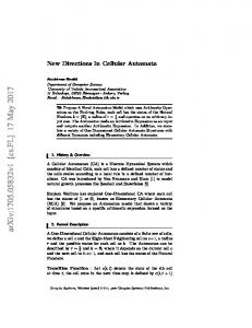
The notion of conceptual structure in cellular automata (CA) rules that perform the density classification task (DCT) was introduced by Marques-Pita et al. (2006). Here we investigate the role of process-symmetry in CAs that solve the DCT, in particular the idea of conceptual similarity, which defines a novel search space for CA rules. We report on two new highest-performing process symmetric rules for the DCT. We further discuss how our results are relevant to understand, control, and design the collective computation performed by other networks of automata, such as those used to model, for example, living systems.

Introduction The intersection of biology and computer science has been a fertile ground for some time. Indeed, Von Neumann was a member of the mid-twentieth century Cybernetics group (Heims, 1991), whose main focus was the understanding of natural and artificial systems in terms of communication and control processes. It is interesting to notice that most early computer science developments were inspired by the models of cognition that orbited this group (e.g. seminal work by McCulloch and Pitts, 1943). Since then, the need to understand how biological systems are able to control and transmit information throughout the huge number of components that comprise them has only increased. Certainly, the study of complex network dynamics has been the subject of a substantial body of literature in the last two decades. From pioneering work on networks of automata (Kauffmann, 1969; Derrida and Stauffer, 1986; Kauffmann, 1993) to more recent systems biology models of gene regulation dynamics (Mendoza and Alvarez-Buylla, 1998; Albert and Othmer, 2003; Espinosa-Soto et al., 2004; Kauffmann, 2003), it is clear that to understand and control the biological organization, it is useful to study the dynamics and robustness of models based on complex networks of automata (Chaves et al., 2005; Willadsen and Wiles, 2007).

Clearly, a novel method for describing and understanding how networks collectively compute, would be welcomed. The work presented here is extremely promising in that regard. The conceptual properties uncovered by our “cognitively-inspired” algorithm provide a more compact and intuitive way to understand how complex networks perform the collective computation that they do. One way to think about the conceptual redescriptions produced by our algorithm is as “dynamical motifs”. Rather than finding common structural network motifs (e.g. Alon, 2007), our redescriptions uncover patterns in the dynamics of automata networks, here specifically the case of cellular automata. Moreover, our redescriptions allow us to understand the global dynamic behavior of novel, high-level conceptual observables built from these redescriptions. In this paper, we focus on a known problem of emergent computation in CA: the density classification task (DCT) (Mitchell et al., 1996). Specifically, we investigate the role of process symmetry, the main conceptual property shared by the majority of CAs that perform the DCT, in (1) defining conceptual spaces where rules with high performance can be found; (2) obtaining more intuitive explanations of the be-

There has been much progress in understanding the structure of natural networks—be it at the level of their scale-free topology (see e.g. Barab´asi, 2002; Newman et al., 2006) or

Artificial Life XI 2008

390

them. These explorations were supported by a cognitivelyinspired method, Aitana (Marques-Pita, 2006). In essence, Aitana takes as input a CA rule in its look-up table form, and outputs the same rule but redescribed in a more compact abstraction. Specifically, the output is a set of schemata that can be used (for example) to reason about the conceptual structure concealed in the look-up table of the input rule. Three of these nine rules have been produced by human engineering: φGKL (Gacs et al., 1978; Gonzaga de S´a and Maes, 1992), φDavis95 and φDas95 (Andre et al., 1996); three were learned with genetic algorithms φDM C (Das et al., 1994) or coevolution methods φCOE1 and φCOE2 (Juill´e and Pollack, 1998). Finally, three of the rules were learned with genetic programming or gene expression programming: φGP 1995 (Andre et al., 1996), φGEP 1 and φGEP 2 (Ferreira, 2001).

havior of rules that perform the DCT; and (3) exploring the process-symmetric vicinity of high performance asymmetric rules. In forthcoming work, we will expand this approach to study other discrete complex networks such as Boolean networks of automata

Cellular Automata A cellular automaton (CA) consists of a regular lattice of N cells. Each cell is in one of k allowed states at a given time t. Let ω ∈ {0, 1, ..., k − 1} denote a possible state of a cell. Let state ω = 0 be referred to as the quiescent state, and any other state as an active state. Each cell is connected to a number of neighbors. Let a local neighborhood configuration (LNC) be denoted by µ, and its size by n. For each LNC in a (n, k) CA an output state is assigned to each cell. This defines a CA rule string, φ, the size of which is k n . In binary CAs, where only two states are allowed(k = 2), it is possible to classify individual cell state-updates in three categories: (1) preservations, where a cell does not change its state in the next time instance t + 1; (2) generations, stateupdates in which the cell goes from the quiescent to the active state; and (3) annihilations, state-updates where the cell goes from the active to the quiescent state. The Initial Configuration (IC) of states of a CA lattice is typically random. The execution of a CA for a number M of discrete time steps, from a given IC, is represented as the set Θ containing M + 1 lattice state configurations.

Marques-Pita et al. (2006) have shown that there is indeed conceptual structure in these CA rules. All of the studied CAs were redescribed in more compact schemata that made explicit certain conceptual properties most of these CAs have in common. Here we studied one of these properties (process-symmetry) in more detail. The next section summarizes the basics of Aitana’s representational redescription architecture, and the conceptual properties found in the studied CAs that perform the DCT.

Aitana: Conceptual Representations of CA

The Density Classification Task (DCT)

Aitana is largely based on a framework for cognitive development in humans: the Representational Redescription Model developed by Karmiloff-Smith (1992), and the Conceptual Spaces framework proposed by G¨ardenfors (2000). There are a number of (recurrent) phases in Aitana’s algorithm: (1) Behavioral Mastery, during which CAs that perform some specific collective computation are learned using, for example, genetic algorithms or coevolution. The learned rules are assumed to be in a representational format we call implicit (conceptual structure is not explicit). (2) Representational Redescription Phase I takes as input the implicit representations (CA look-up tables) and attempts to compress them into explicit-1 (E1) schemata by exploiting structural regularities within the input rules. (3) Phase II (and beyond) look for ways to further compress E1 representations, for example by looking at how groups of cells change together, and how more complex schemata are capable of generating regular patterns in the dynamics of the CA. The focus in this paper is on Phase I redescription.

The Density Classification Task (DCT) is one of the most studied examples of collective computation in cellular automata. The goal is to find a binary CA rule that can best classify the majority state in the randomized IC. If the majority of cells in the IC are in the quiescent (active) state, after a number of time steps M , the lattice should converge to a homogeneous state where every cell is in the quiescent (active) state. Since the outcome could be undecidable in lattices with even number of cells (N ), this task is only applicable to lattices with an odd number of cells. Devising CA rules that perform this task is not trivial, because cells in a CA lattice update their states based only on local neighborhood information. However, in this particular task, it is required that information be transferred across time and space in order to achieve a correct global classification. The definition of the DCT used in our studies is the same as the one by Mitchell et al. (1993). The nine highest-performing 1-dimensional CA rules that perform the DCT were analyzed by Marques-Pita et al. (2006). The goal of that analysis was to determine whether there is conceptual structure in these rules, and in that case, to investigate the possible conceptual similarity among

Artificial Life XI 2008

E1 representations are produced by modules in Aitana. Here we focus on the Wildcard module. The CA rules studied were redescribed with the this module, introduced in the next section.

391

Conceptual properties of CAs for the DCT

The Wildcard Module

One of the main novel findings reported in Marques-Pita et al. (2006) is the fact that most rules that perform the density classification task are process-symmetric. Process symmetry for binary CA rules is defined as a bijective mapping between the members of the only two possible sets of schemata prescribing state changes: generation processes, which refer to a cell state change from ω = 0 to ω = 1, and annihilation processes which refer to the reverse state change.

This module uses regularities in the set of entries—one for each possible LNC—of a CA’s look-up table, in order to produce E1 representations captured by wildcard schemata. These schemata are defined in the same way as the look-up table entries for each LNC of a CA rule, but allowing an extra symbol to replace the state of one or more cells within them. This new symbol is denoted by “#”. When it appears in a E1 schema it means that in the place where it appears, any of the possible k states is accepted. The idea of using wildcards in representational structures was first proposed by Holland et al. (1986), when introducing Classifier Systems. The wildcard redescriptions used here are Processspecific, i.e. they do not allow a wildcard symbol in the place of an updating cell in a schema. This makes it possible for them to describe processes in the CA rule unambiguously. For example, a generation, schema {#, #, #, 0, 1, #, 1} prescribes that a cell in state ω = 0, with immediate-right and end-right neighbors in state ω = 1 updates its state to ω = 1 regardless of the state of the other neighbors.

Using the concept of process symmetry, one can easily define a function that converts a generation into an annihilation process, and vice versa. Such a function of E1 redescriptions, transforms a schema s into its corresponding process-symmetric schema s0 by (1) reversing the elements in s using a mirror function M (s), and (2) exchanging ones for zeros, and zeros for ones (leaving wildcards untouched), using a negation function N (s). Thus, in every process symmetric CA rule, given the set S = {s1 , s2 , ..., sz } of all schemata si prescribing a state-change process, the elements of the set of schemata prescribing the converse process S 0 = {s01 , s02 , ..., s0z } can be found by applying the bijective mapping between processes defined by the composition s0i = (M ◦ N )(si ). This property is illustrated in Figure 1, where the E1 schemata of the process symmetric rule φGP 1995 (Andre et al., 1996) are shown.

The implementation of the wildcard module in Aitana consists of a simple McCulloch and Pitts neural network. In this assimilation network, input units represent each lookup table entry (one for each LNC), and ouput units represent all the possible schemata available to redescribe segments of the input rule (see Marques-Pita, 2006, for details).

Assimilation and Accommodation Phase I redescription in Aitana depends on two interrelated mechanisms, assimilation and accommodation1 . During Phase I, the units in the input layer of an assimilation network are activated to reflect the output states in the input CA rule to be processed. The firing of these units spreads, thus activating other units across the network. When some unit in the network (representing a E1 schema) has incoming excitatory fibers above a threshold it fires. This firing signals that the schema represented by the unit becomes an E1 redescription of the lower level units that caused its activation. When this happens, inhibitory signals are sent back to those lower level units so that they stop firing (since they have been redescribed). At the end of assimilation, the units that remain firing represent the set of wildcard schemata redescribing the input CA rule. Once the process of assimilation has been completed, Aitana will try to “force” the assimilation of any (wildcard-free) look-up table entry that was not redescribed i.e. any input unit that is still firing. This corresponds to the accommodation process implemented in Aitana (see Marques-Pita, 2006, for further details).

Generation

Annihilation

ϕGP1995

{#, #, #, 0, 1, #, 1} {#, #, 1, 0, #, #, 1} {1, #, #, 0, #, #, 1}

{0, #, 0, 1, #, #, #} {0, #, #, 1, 0, #, #} {0, #, #, 1, #, #, 0}

Figure 1: E1 schemata prescribing state changes for φGP 1995 . Any annihilation (right column) can be obtained by reversing the corresponding generation schema (to the left), and exchanging zeros for ones, and ones for zeros. Six out of the nine rules analyzed by Marques-Pita et al. were found to be process-symmetric. The remaining three, φCOE1 and φCOE2 and φDM C are not. It is interesting to note that the three non processsymmetric rules were discovered via evolutionary algorithms (GAs and coevolutionary search) which apply variation to genetic encodings of the look-up tables of CAs. Therefore, genotype variation in these evolutionary algorithms operates at the low level of the bits of the look-up table—what we referred to as the implicit representation of a CA. In contrast, the other forms of search of design that lead to the other six (process-symmetric) rules, while not looking explicitly for process symmetry, were based on mechanisms and reasoning trading in the higher-level behavior and

1 These two processes are inspired in those defined by Piaget in his theory of Constructivism (see e.g. Piaget, 1952, 1955)

Artificial Life XI 2008

RULE

392

structure of the CA—what we refer to as the explicit representation of a CA. Marques-Pita et al. have also determined that it is possible to define conceptual similarity between the process symmetric CA rules for the DCT. For example, the rule φGP 1995 can be derived from φGKL . Moreover, the best process-symmetric rule known for this task (at the time) was found via conceptual transformations: φM M 401 2 with per105 ≈ 0.833 . However, the performance of this formance P149 rule is still below the performance of the best CA rule for 105 ≈ 0.86. the DCT, namely φCOE2 , with P149

RULE

Generation

Annihilation

ϕMM0711

{#, #, 0, 0, #, 1, 1} {1, #, #, 0, #, 1, 1} {1, 0, #, 0, 1, #, #} {1, #, 1, 0, #, #, #}

{0, 0, #, 1, 1, #, #} {0, 0, #, 1, #, #, 0} {#, #, 0, 1, #, 1, 0} {#, #, #, 1, 0, #, 0}

Figure 2: E1 schemata prescribing state changes for the CA rule φM M 0711 . This CA is process-symmetric.

Process-Symmetry in φCOE2 The 4-Wildcard Process-Symmetric Space

Figure 3 shows the state-change schema sets for φCOE2 . 105 The performance of this rule is P149 ≈ 0.86. We tested this 5 rule on two sets of 10 ICs, one with majority ω = 0, the other with majority ω = 1. Samples were taken from binomial dist. centered around 0.5 (most difficult cases to clas105 sify). The performances were, respectively, P149 ≈ 0.83 5 10 and P149 ≈ 0.89. Thus, even though on average this is the best CA rule for the DCT, it performs much better when there is a majority of “1’s” in the ICs.

Starting with the conceptual similarities previously observed between φGKL and φGP 1995 , we now report a search of the “conceptual space” where these two CA rules can be found: the space of process-symmetric binary CA rules with neighborhood size n = 7, where all state-change schemata have four wildcards. A form of evolutionary search was used to evaluate rules in this space as follows: the search starts with a population of sixty-four different process-symmetric rules containing only 4-wildcard schemata; the generation and annihilation schema sets for an individual were allowed to have any number of schemata in the range between two and eight; crossover operators were not defined; a mutation operator was set, allowing the removal or addition of up to two randomly chosen 4-wildcard schemata (repetitions not allowed), as long as a minimum of two schemata are kept in each schema set; in every generation the fitness of each member of the population is evaluated against 104 ICs, keeping the top 25% rules (elite) for the next generation without modification; offspring are generated by choosing a random member of the elite, and applying the mutation operator until completing the population size with different CA rules; a run consisted of 500 generations, and the search was executed for 8 runs. There are 60 possible 4-wildcard processsymmetric schemata-pairs. Thus, our search space contains approximately 3 × 109 rules defined by generation and annihilation schema sets of size between 2 and 8.

Generation

Annihilation

ϕCOE2

g1 {1, 0, 1, 0, #, #, #} g2 {1, 0, #, 0, #, 1, 1} g3 {1, 1, #, 0, 1, #, #} g4 {1, #, 1, 0, 1, #, #} g5 {1, #, 1, 0, #, 0, #} g6 {1, #, #, 0, 1, 1, #} g7 {1, #, #, 0, 1, #, 1} g8 {#, 0, 0, 0, 1, 0, 1} g9 {#, 0, 1, 0, 0, 1, #} g10 {#, 0, #, 0, 0, 1, 1} g11 {#, 1, 1, 0, 1, #, 0} g12 {#, 1, 1, 0, #, 0, #}

a1 {0, 0, 1, 1, 1, 1, #} a2 {0, 0, #, 1, #, 1, 0} a3 {0, 1, 0, 1, 1, #, #} a4 {0, #, 0, 1, #, #, 0} a5 {1, 0, 0, 1, #, 0, #} a6 {#, 0, 0, 1, #, #, 0} a7 {#, #, 0, 1, 1, 0, #} a8 {#, #, 0, 1, #, 0, 0} a9 {#, #, #, 1, 0, #, 0}

Figure 3: E1 schemata prescribing state changes for φCOE2 . This is the highest-performing rule for the DCT. φCOE2 is not process-symmetric. We claim that this divergence in behavior is due to the fact that φCOE2 is not process-symmetric. Evaluation of split performance on the ten best rules for the DCT supports this hypothesis (see Table 1). The difference between the two biased performance measures for the non-process-symmetric rules is one or two orders of magnitude larger than for the process-symmetric rules. This indicates that process symmetry seems to lead to more balanced rules—those that respond equally well to both types of of problem.

Our search found one rule with better performance than 105 φM M 401 . This rule, φM M 0711 4 has P149 ≈ 0.8428. The state-change schema sets for this rule are shown in Figure 2. Even though this search resulted in an improvement, the performance gap between the best process-symmetric rule, φM M 0711 and φCOE2 is still close to 2%. Is it possible then, that a process-symmetric rule exists “hidden” in the conceptually “messy” φCOE2 ?

It is then reasonable to ask: Is there a process-symmetric rule in the conceptual vicinity of φCOE2 , whose performance is as good (or higher) than the performance φCOE2 ? To answer this question we pursued a number of tests. First, we looked at the CA rule resulting from keeping all annihilations in φCOE2 , and using only their process-symmetric 105 generations. The performance of that rule was P149 ≈ 0.73.

2 In inverse lexicographical hexadecimal format, φM M 401 is ffaaffa8ffaaffa8f0aa00a800aa00a8 3 105 The measure P149 refers to the proportion of correct classifi5 cations in 10 ICs of length 149 4 In inverse lexicographical hexadecimal format, φM M 0711 is faffba88faffbaf8fa00ba880a000a88

Artificial Life XI 2008

RULE

393

10

5

P 149

M→0

10

5

P 149

M→1

binary matrix representation in Figure 4 be denoted by A, where all shaded elements in the figure represent 1s and the rest are 0s. In the figure the lighter colored matrix elements are used to distinguish annihilation processes from generation processes, which are shown in a darker color.

P. DIFF.

ϕGKL

0.8135

0.8143

0.0008

ϕDavis95

0.8170

0.8183

0.0013

ϕDas95

0.8214

0.8210

0.0004

ϕGP1995

0.8223

0.8245

0.0022

ϕDMC

0.8439

0.7024

0.1415

ϕCOE1

0.8283

0.8742

0.0459

ϕCOE2

0.8337

0.888

0.0543

ϕGEP1

0.8162

0.8173

0.0011

ϕGEP2

0.8201

0.8242

0.0041

ϕMM0711

0.8428

0.8429

0.0001

Given the ordering of elements in the columns of Figure 4, if a generation row is isolated, and then reversed, the result can be matched against any of the annihilation rows to calculate the total degree of process symmetry between the two schemata represented in the two rows. A total match means that the original generation schema is processsymmetric with the matched annihilation schema. A partial match indicates a degree of process symmetry. This partial match can be used by Aitana’s accommodation mechanism to force the highly process-symmetric pair into a fully process-symmetric one, keeping the modified representation only if there is no loss of performance.

Table 1: Split performances of the ten best DCT rules. Darker rows correspond to process-symmetric rules; white rows refer to non-process-symmetric rules. For the latter, there is a significant difference in performance: φDM C is better at classifying cases where state 0 is in the majority; φCOE1 and φCOE2 are considerably better at solving the problem when state 1 is in the majority. The difference between the split performance measures is one to two orders of magnitude larger for the non-process-symmetric rules.

More concretely, the degree of process symmetry existing between two schemata Sg and Sa prescribing opposite processes (a generation schema, and an annihilation respectively) is calculated as follows: 1. Pick rows Sg and Sa from matrix A such that Sg corresponds to a generation and Sa to an annihilation.

A second test was the reverse of the first one: keeping all generations of φCOE2 , and using only their processsymmetric annihilations. The resulting rule has a perfor105 mance P149 ≈ 0.47.

2. Reverse one of the rows (e.g. Sa ). This makes it possible to compare each LNC (the columns) with its processsymmetric pair, by looking at the ith element of each of the two row vectors.

For the next test, we looked at the degree of process symmetry already existing in φCOE2 . To find this we used the matrix-form representation of φCOE shown in Figure 4. Each column contains each of the 128 LNCs for a onedimensional binary CA rule and neighborhood radius three. These LNCs are not arranged in lexicographical order, instead they are arranged as process-symmetric pairs: the first and last LNCs are process-symmetric, the second, and next to last are also process-symmetric and so on, until the two LNCs in the center are also process-symmetric. Each row corresponds to the E1 (wildcard) state-changing schemata for φCOE2 . The first nine rows correspond to the annihilation schemata, and the subsequent ones the twelve generation schemata for φCOE2 .

3. Calculate the degree of process symmetry as: 2 × Sg · Sa |Sg | + |Sa | where, the dot product of binary vectors, Sg · Sa is the number of component-matches; and |S| is the number of ones in a binary vector.5 All the generation rows were matched against all the annihilation rows in matrix A, recording the proportion of matches found. Table 2 shows the results of this matching procedure (only highest matches shown). The darker rows correspond to schema pairs that are fully process-symmetric. The first three light gray rows (with matching score 66%) show an interesting, almost complete process symmetry subset, involving generation schemata g1, g4 and g5, and annihilation schema a9.

In any of the first nine rows, a shaded-cell represents two things: (1) that the LNC in that column is an annihilation; and (2) that the LNC is part of the E1 schema labeled in the row where it appears. The twelve rows for generation schemata are reversed. This makes it simple to inspect visually what process-symmetric LNCs are present in the rule, which is the case when for a given column, there is, at least, one cell shaded in one of the first nine rows (an active annihilation), and at least one cell shaded in one of the bottom nine rows (an active generation). Let the schemata × LN C

Artificial Life XI 2008

Using the accommodation mechanism in Aitana, we “generalized” the schemata g1, g4 and g5 into the more general process symmetric pair of a9 (that encompasses 5

While |x| is the notation typically used for cardinality of sets, here, we use it to represent the 1-norm, more commonly denoted by ||x||1 .

394

a3 a5 a7 a9

g9 g10 g11 g12

Figure 4: E1 processes for φCOE2 , without the preservations. Here, the generation rows have been reversed, so that it becomes much easier to determine what LNCs do not have their process-symmetric LNC active. The dotted vertical lines show these LNCs. Each of these state-change prescriptions were removed in φCOE2clean .

The last test to be reported consisted in evaluating the CA rules derived from (1) taking φCOE2−clean as base (each time); (2) adding to it a number of process symmetric pairs from R to it; and (3) evaluating the resulting CA rule. This set contains all CA rules that are the same as φCOE2−clean , but adding one of the twelve pairs in R; it also contains all the rules that are as φCOE2−clean , including combinations of two pairs from R (66 rules), and so on. The total number of CA rules derived in this way is 40966 .

Matching score

Generation schemata

Annihilation schemata

g1

a9

66%

g2

a2

100%

g3

a8

100%

g4

a9

66%

g5

a9

66%

g6

a6

100%

g7

a4

100%

g8

a3

66%

g9

a2

25%

g10

a1

66%

g11

a5

50%

g12

a9

33%

The performance of the 4096 rules is shown in Figure 6. Each column shows the performance of the subsets of rules adding one pair of LNCs from R, subsets adding combinations of two pairs, and so on. Note that the median performance in each subset decreases for rules containing more pairs of LNCs from R. However, the performance of the best CA rules in each subset increases for all subsets including up to six LNC pairs, and then decrease.

Table 2: Degree of process symmetry amongst all the generation and annihilation schemata in φCOE2 . Gray rows indicate full process symmetry, pink rows indicate a high degree of process symmetry

the three of them), and tested the resulting CA rule. We also “specialized” by breaking a9 into the three processsymmetric schemata of g1, g4 and g5, with performance , 105 P149 < 0.6 in both cases.

One of the tested CAs, containing six LNC pairs added to φCOE2−clean , is the best process-symmetric CA for the 105 DCT with P149 ≈ 0.85. The schemata for this CA, φM M 0802 , are shown in Figure 7. φM M 0802 , has a performance that is very close to that of the second highestperforming rule known for the DCT, φCOE1 (see MarquesPita et al., 2006). However, φM M 0802 is the highestperforming CA for split performance for the DCT—which means that it classifies correctly the two types of IC it can encounter (majority 1s or majority 0s).

Still working with the degree of process-symmetry in φCOE2 , it is possible to extract a matrix representation A0 , containing only those LNC process-symmetric pairs in A. In other words, each column in A0 will be exactly as in A, as long as the column contains 1s for at least one annihilation and one generation row, otherwise the column is all 0s (the latter is the case for all columns marked with dotted lines in Figure 4). We will refer to the rule represented by the matrix A0 as φCOE2−clean —the CA rule that preserves all the process symmetry in φCOE2 . The “orphan” LNCs removed from A are shown in Figure 5 (white background). Their process-symmetric pairs are in the same Figure (gray background). We will refer to this set of LNC pairs as R.

Artificial Life XI 2008

6

Note that each of the rules tested comes from adding a particular combination of pairs each time to the original φCOE2−clean , as opposed to adding pairs of LNCs cumulatively to φCOE2−clean .

395

Generation

Annihilation

{0, 1, 1, 0, 1, 0, 1} {0, 1, 1, 0, 1, 0, 0} {0, 1, 1, 0, 0, 0, 1} {0, 1, 1, 0, 0, 0, 0} {0, 0, 1, 0, 0, 1, 1} {0, 0, 1, 0, 0, 1, 0}

{0, 1, 0, 1, 0, 0, 1} {1, 1, 0, 1, 0, 0, 1} {0, 1, 1, 1, 0, 0, 1} {1, 1, 1, 1, 0, 0, 1} {0, 0, 1, 1, 0, 1, 1} {1, 0, 1, 1, 0, 1, 1}

{0, 1, 0, 0, 1, 1, 1} {1, 1, 1, 0, 0, 1, 1} {1, 1, 1, 0, 0, 1, 0} {0, 1, 0, 0, 1, 1, 0} {0, 1, 0, 0, 1, 0, 1} {0, 1, 0, 0, 1, 0, 0}

{0, 0, 0, 1, 1, 0, 1} {0, 0, 1, 1, 0, 0, 0} {1, 0, 1, 1, 0, 0, 0} {1, 0, 0, 1, 1, 0, 1} {0, 1, 0, 1, 1, 0, 1} {1, 1, 0, 1, 1, 0, 1}

Annihilation

ϕMM0802

{1, 0, 1, 0, #, #, #} {1, 0, #, 0, #, 1, 1} {1, 1, #, 0, 1, #, #} {1, #, 1, 0, 1, #, #} {1, #, 1, 0, #, 0, #} {1, #, #, 0, 1, 1, #} {1, #, #, 0, 1, #, 1} {#, 0, 0, 0, 0, 1, 1} {#, 1, 0, 0, 1, #, #} {#, 1, #, 0, 1, 0, #} {#, 1, #, 0, 1, #, 0} {#, #, 0, 0, 1, 0, 1}

{0, 0, 1, 1, 1, 1, #} {0, 0, #, 1, #, 1, 0} {0, 1, 0, 1, 1, #, #} {0, #, 0, 1, #, #, 0} {1, #, 0, 1, #, 0, #} {#, 0, 0, 1, #, #, 0} {#, 1, 0, 1, #, 0, #} {#, 1, #, 1, 0, #, 0} {#, #, 0, 1, 0, #, 0} {#, #, 0, 1, 1, 0, #} {#, #, 0, 1, #, 0, 0} {#, #, #, 1, 0, 1, 0}

are not claiming process-symmetry is the important discovery per se. Instead, the result we consider to be an important advance is the discovery of conceptual structure in a form of complex network—since, by representing concepts (e.g. process-symmetry), it becomes possible to reason about collective computation in new, less perplexing ways.

1.0

0.8

Performance

Generation

Figure 7: Schemata prescribing state changes for φM M 0802 , the best process-symmetric rule for the DCT.

Figure 5: The set R of twelve LNCs in φCOE2 (white background) for which their corresponding process-symmetric LNCs are preservations in the original CA rule (italics).

0.6

0.4

Here we showed that the ability to redescribe the dynamics of automata networks into a form that is both easier to understand and to search for new robust behaviors, was very useful for the DCT and CA rules at large. Our results indicate that there seems to exist conceptual structure in the dynamics of networks of automata that perform collective computation. But it should be emphasized that our methodology is not applicable only to CAs and the DCT; it is applicable the study of other complex networks of automata. We are currently exploring the conceptual structure in biochemical networks modeled using Boolean networks. If we can understand the dynamics of, say, a gene regulation network as a form of computation and we uncover the dynamical motifs responsible for that computation, not only do we gain a greater insight about the function of the network, but we can also discover similar network configurations that can be more robust, or those that lead to alternate behaviors more easily. This could prove useful in understanding phylogenetic differences, or differences from wild-type phenotypes. Thus, while here we only present results for the DCT in CA, the approach is quite relevant for both Artificial Life and Computational Biology.

0.2

0.0

RULE

1 p. 2 p. 3 p. 4 p. 5 p. 6 p. 7 p. 8 p. 9 p. 10 p. 11 p. 12 p.

Process-symmetric tested sets

Figure 6: Performances of the 4096 process-symmetric CAs in the immediate conceptual vicinity of φCOE2 . The best specimen CA is φCOE2c lean plus one of the combinations of 6 process-symmetric pairs from R.

Conclusions and Discussion Besides the two new best process-symmetric CA rules for the DCT, perhaps the most important conclusion from this work is concerned with the fact that representational redescription gives us a new method to relate the local interactions of automata in networks, to the dynamic patterns of collective computation of the network as a whole. Indeed, this constitutes an unexpected advance. When working with implicit CA rules and genetic algorithms, Mitchell et al. (1993) noted that there is no geometry in the space of CA rules represented as look-up state transition tables. Specifically, there was no way of knowing the effect of changing one output in the rule table on its ability to perform a specific collective computation. However, using the conceptually redescribed search spaces we explored here, this is clearly not the case. Conceptual manipulations of CAs in this space result in CAs with similar dynamics—although not necessarily always high performance (Marques-Pita et al., 2006). We

Artificial Life XI 2008

Acknowledgements We would like to thank Melanie Mitchell for valuable comments. This work was partially supported by Fundac.a˜ o para a Ciˆencia e a Tecnologia (Portugal) grant 36312/2007. We also thank the FLAD Computational Biology Collaboratorium at the Gulbenkian Institute (Portugal) for hosting and providing facilities used for part of this research.

396

References

Karmiloff-Smith, A. (1992). Beyond Modularity: A Developmental Perspective on Cognitive Science. MIT Press.

Albert, R. and Othmer, H. (2003). The topology of the regulatory interactions predicts the expression pattern of the segment polarity genes in drosophila melanogaster. J Theor Biol, 223(1):1–18.

Kauffmann, S. (1969). Metabolic stability end epigenesis in randomly constructed genetic nets. Journal of Theoretical Biology, 22:437–467. Kauffmann, S. (1993). The Origins of Order: Self-Organization and Selection in Evolution. Oxford University Press.

Alon, U. (2007). Network motifs: theory and experimental approaches. Nat Rev Genet, 8(6):450–461.

Kauffmann, S. (2003). Random Boolean network models and the yeast transcriptional network. Proc Natl Acad Sci U S A, 100(25):14796–14799.

Andre, D., III, F. B., and Koza, J. (1996). Discovery by genetic programming of a cellular automata rule that is better than any known rule for the majority classification problem. In Koza, J., Goldberg, D., and Fogel, D., editors, Proceedings of the First Annual Conference on Genetic Programming, pages 3–11. MIT Press.

Marques-Pita, M. (2006). Aitana: A Developmental Cognitive Artifact to Explore the Evolution of Conceptual Representations of Cellular Automata-based Complex Systems. PhD thesis, School of Informatics, University of Edinburgh, Edinburgh, UK.

Barab´asi, A.-L. (2002). Linked: The New Science of Networks. Perseus Books, New York, USA.

Marques-Pita, M., Manurung, R., and Pain, H. (2006). Conceptual representations: What do they have to say about the density classification task by cellular automata? In Jost, J., ReedTsotchas, F., and Schuster, P., editors, ECCS’06, European Conference on Complex Systems.

Chaves, M., Albert, R., and Sontag, E. D. (2005). Robustness and fragility of boolean models for genetic regulatory networks. J Theor Biol, 235(3):431–449. Das, R., Mitchell, M., and Crutchfield, J. (1994). A genetic algorithm discovers particle-based computation in cellular automata. In Davidor, Y., Schwefel, H. P., and M¨anner, R., editors, Proceedings of the Int.Conf. on Evolutionary Computation., pages 344–353.

McCulloch, W. and Pitts, W. (1943). A logical calculus of ideas immanent in nervous activity. Bulletin of Mathematical Biophysics, 5:115–133. Mendoza, L. and Alvarez-Buylla, E. R. (1998). Dynamics of the genetic regulatory network for arabidopsis thaliana flower morphogenesis. J Theor Biol, 193(2):307–319.

Derrida, B. and Stauffer, D. (1986). Phase transitions in twodimensional Kauffmann cellular automata. Europhys. Lett., 2:739–745.

Mitchell, M. (2006). Complex systems: Network thinking. Artificial Intelligence, 170(18):1194–1212.

Espinosa-Soto, C., Padilla-Longoria, P., and Alvarez-Buylla, E. R. (2004). A gene regulatory network model for cell-fate determination during arabidopsis thaliana flower development that is robust and recovers experimental gene expression profiles. Plant Cell, 16(11):2923–2939.

Mitchell, M., Crutchfield, J., and Das, R. (1996). Evolving cellular automata with genetic algorithms: A review of recent work. In Proceedings of the First International Conference on Evolutionary Computation and its Applications (EvCA’96). Russian Academy of Sciences.

Ferreira, C. (2001). Gene expression programming: A new adapive algorithm for solving problems. Complex Systems, 13(2):87– 129.

Mitchell, M., Crutchfield, J., and Hraber, P. (1993). Revisiting the edge of chaos: Evolving cellular automata to perform computations. Complex Systems, 7:89–130.

Gacs, P., Kurdyumov, L., and Levin, L. (1978). One-dimensional uniform arrays that wash out finite islands. Probl. Peredachi. Inform., 14:92–98.

Newman, M., Barab´asi, A.-L., and Watts, D. J. (2006). The Structure and Dynamics of Networks. Princeton University Press, Princeton, NJ.

G¨ardenfors, P. (2000). Conceptual Spaces: The Geometry of Tought. MIT Press/Bradford Books.

Peak, D., West, J. D., Messinger, S. M., and Mott, K. A. (2004). Evidence for complex, collective dynamics and distributed emergent computation in plants. In Proceedings of the National Academy of Science, volume 101, pages 918–922.

Gonzaga de S´a, P. and Maes, C. (1992). Gacs-Kurdyumov-Levin automaton revisited. Journal of Statistical Physics, 67(34):507–522. Heims, S. J. (1991). The Cybernetics Group. MIT Press.

Piaget, J. (1952). The Origins of Intelligence in Children. International University Press.

Helikar, T., Konvalina, J., Heidel, J., and Rogers, J. A. (2008). Emergent decision-making in biological signal transduction networks. Proc Natl Acad Sci U S A, 105(6):1913–1918.

Piaget, J. (1955). The Child’s Construction of Reality. Routledge and Kegan Paul.

Holland, J., Holyoak, K., Nisbett, R., and Thagard, P. (1986). Induction: Processes of Inference, Learning and Discovery. MIT Press.

Willadsen, K. and Wiles, J. (2007). Robustness and state-space structure of boolean gene regulatory models. J Theor Biol, 249(4):749–765.

Juill´e, H. and Pollack, B. (1998). Coevolving the ideal trainer: Application to discovery of cellular automata rules. In Garzon, M. H., Goldberg, D. E., Iba, H., and Riolo, R., editors, Genetic Programming 1998: Proceedings of the Third Annual Conference, San Francisco. Morgan Kauffmann.

Artificial Life XI 2008

397