Condition-dependent functional connectivity: syntax networks in ...

Phil. Trans. R. Soc. B (2005) 360, 921–935 doi:10.1098/rstb.2005.1653 Published online 29 May 2005

Condition-dependent functional connectivity: syntax networks in bilinguals Silke Dodel1,*, Narly Golestani2, Christophe Pallier1,2, Vincent ElKouby1, Denis Le Bihan1 and Jean-Baptiste Poline1,3,* 1

2

Service Hospitalier Fre´de´ric Joliot, CEA, IFR49, 91401 Orsay, France Inserm U562 Cognitive neuroimaging unit, 3Inserm ERM 02-05 Neuroimaging in psychiatry, SHFJ, IFR49, 91401 Orsay, France

This paper introduces a method to study the variation of brain functional connectivity networks with respect to experimental conditions in fMRI data. It is related to the psychophysiological interaction technique introduced by Friston et al. and extends to networks of correlation modulation (CM networks). Extended networks containing several dozens of nodes are determined in which the links correspond to consistent correlation modulation across subjects. In addition, we assess inter-subject variability and determine networks in which the condition-dependent functional interactions can be explained by a subject-dependent variable. We applied the technique to data from a study on syntactical production in bilinguals and analysed functional interactions differentially across tasks (word reading or sentence production) and across languages. We find an extended network of consistent functional interaction modulation across tasks, whereas the network comparing languages shows fewer links. Interestingly, there is evidence for a specific network in which the differences in functional interaction across subjects can be explained by differences in the subjects’ syntactical proficiency. Specifically, we find that regions, including ones that have previously been shown to be involved in syntax and in language production, such as the left inferior frontal gyrus, putamen, insula, precentral gyrus, as well as the supplementary motor area, are more functionally linked during sentence production in the second, compared with the first, language in syntactically more proficient bilinguals than in syntactically less proficient ones. Our approach extends conventional activation analyses to the notion of networks, emphasizing functional interactions between regions independently of whether or not they are activated. On the one hand, it gives rise to testable hypotheses and allows an interpretation of the results in terms of the previous literature, and on the other hand, it provides a basis for studying the structure of functional interactions as a whole, and hence represents a further step towards the notion of largescale networks in functional imaging. Keywords: functional connectivity; psychophysiological interaction; network; fMRI; syntax; bilinguals

1. INTRODUCTION Functional magnetic resonance imaging (fMRI) studies are often criticized as being mostly performed in the spirit of neophrenology, that is, aiming to describe the locations in the brain where the signal varies, along with an externally induced paradigm, but not being capable of describing the functional links or interactions between these regions (e g. Fodor 1999). The regions identified in this manner are often referred to as the network activated by a given contrast of experimental conditions, yet often, little is said about how the strength of the functional links between these regions vary with experimental conditions (Friston et al. 2002). At the simplest level, connectivity analyses may reveal differences in the brain functional organization not detectable with direct comparisons of

activity induced by experimental conditions. For instance, the same regions may be activated in bilinguals processing sentences in their first or second language (Perani et al. 1998), but there may be differences between the two languages in the strength of functional connections between the areas involved. In this paper, we present a method to examine variations in functional connectivity across experimental conditions, and we apply it to fMRI data on sentence production in the first and the second language in bilinguals. The results of previous functional imaging studies on bilingualism are not entirely consistent. Several studies suggest that the neural circuitry for the first (L1) and second languages (L2) is shared (Klein et al. 1994, 1995; Perani et al. 1998; Chee et al. 1999a,b), while other studies have found a different pattern of activation for L1 and L2 (Dehaene et al. 1997; Kim et al. 1997). Age of acquisition and level of proficiency of the subjects are variables that may explain the discrepancies between the studies

* Authors for correspondence([email protected], [email protected]). One contribution of 21 to a Theme Issue ‘Multimodal neuroimaging of brain connectivity’.

921

q 2005 The Royal Society

922

S. Dodel and others Connectivity networks in bilinguals

(see Abutalebi et al. 2001; for a review). In the present study, late bilinguals with varying levels of proficiency in L2 were scanned while seeing series of words written either in the first (L1) or in the second language (L2). In a first condition, they had to simply read the words; in another condition, they had to build a simple sentence out of them. The comparison between these two conditions ought to reveal processes involved in sentence building and syntactical processing. Note, however, that syntactical processing is not isolated in this comparison, and that other processes such as semantic evaluation and lexical selection are probably also revealed. Given that the tasks involved word reading and syntactical production, below we briefly review some imaging studies on word reading and on syntax processing. (a) Background on word reading and syntax studies Functional neuroimaging studies on word reading suggest that different regions are involved in different aspects of word reading. For example, occipital and fusiform regions are thought to be involved in the processing of written words, while the left frontal operculum, inferior frontal cortex and insula are thought to be involved in phonological analysis, verbal short term memory and articulation, and the primary motor cortex (BA 4), the precentral gyrus, the supplementary motor area (SMA) and the cerebellum probably contribute to the motoric and premotoric aspects of speech production. Regions such as Broca’s area, in the left inferior frontal gyrus (LIFG), and Wernicke’s area, in the posterior temporal and inferior parietal regions, are thought to contribute to aspects of processing that are ‘linguistic’ per se. Most neuroimaging studies specifically examining syntactic processing have found activation in Broca’s area in the left inferior frontal cortex (BA 44/45; Just et al. 1996; Caplan et al. 1998; Dapretto & Bookheimer 1999; Embick et al. 2000; Friederici et al. 2000; Ni et al. 2000; Sakai et al. 2002). Activation has also been shown in other brain regions, including the anterior temporal lobe, the left or bilateral superior and middle temporal gyri (BA 21/22), the left inferior parietal cortex, the cingulate gyrus, and finally, the basal ganglia (Fiebach et al. 2001; Keller et al. 2001; Cooke et al. 2002). Note that Broca’s area is probably not syntax-specific, as it has been shown to be activated during a variety of other tasks. Some recent studies have addressed the functional connections, or variations in these, during or across language tasks. For example, Hampson et al. (2002) measured functional connectivity between regions of interest (ROI) during continuous listening, and compared it to the connectivity found during the resting state, and found connection between Broca’s area and Wernicke’s area at rest. Similar work has been carried out by Waites et al. (2004), who showed increased connectivity between the left and right middle frontal gyri in a language production task, or by Bokde et al. (2001), who showed a functional parcelling of the LIFG in terms of its links with posterior brain regions. There is a key distinction between correlations measured in steady-state1 data and correlations evoked Phil. Trans. R. Soc. B (2005)

by experimental design. The above studies mostly looked at correlations during a particular task or brain state (i.e. steady-state correlations), allowing one to attribute the correlations to a specific brain state. However, these correlations result from experimentallyuncontrolled variations around the average steadystate, and contributions of subject’s movement and physiological artefacts are not easily assessed. Therefore, their causes are unknown and their interpretation is difficult. Hence, many other studies have taken a different route and assessed the variation in connectivity strength across experimental conditions (among others, see Mechelli et al. 2002; He et al. 2003; Horwitz & Braun 2004; Just et al. 2004). In particular, Just et al. (2004) recently report variation in connectivity between lowand high-imagery sentences, presented visually or auditorily, between the left intraparietal sulcus and language processing cortical areas. Effective connectivity studies fall in this class of methods, and have been recently extended to incorporate inter-subject variability by Mechelli et al. (2002), who reported that the effect of word type (actual or pseudo words) on reading-related coupling differed significantly among subjects. Nevertheless, work on functional or effective connectivity of language networks, in particular in its attempt to further understanding of bilingualism, is still at a very early stage. In this study, we attempt to overcome some of the current limitations of functional connectivity methods (see §1b) using a semi-exploratory approach, and to bring new insights into the mechanisms of language production in the context of bilingualism. (b) Functional and effective connectivity methods: a quick review Connectivity analyses that search for inter-regional interactions can be approximately divided into methods that create functional connectivity maps, often performed with steady state paradigms (positron emission tomography (PET) or fMRI), and methods that are based on an a priori anatomical model of the connections and assess the strength of these during different experimental conditions. While the former methods are more exploratory and aim at finding new nodes in the brain networks sustaining one or several cognitive processes, the latter are more inferential and allow the assessment of effective connectivity as defined by Friston (1994). Works of the first kind can be found, among many others, in (Horwitz et al. 1984; Metter et al. 1984; Bartlett et al. 1987; Biswal et al. 1995, 1997; Golay et al. 1998; Horwitz et al. 1998; Tononi et al. 1998; Goutte et al. 1999; Cordes et al. 2000; Lohmann & von Cramon 2001; Cordes 2002; Muller et al. 2002), while the second framework was initially developed in neuroimaging with PET by McIntosh & Gonzalez-Lima (1994), Friston (1994), Grafton et al. (1994) and McIntosh & Gonzalez-Lima (1995), and further extended and applied to fMRI data in, for instance, Bu¨chel & Friston (1997), Buchel & Friston (1998), Friston et al. (2003). For a general review on functional or effective connectivity issues, see Horwitz (2003) and Bullmore et al. (2004). The construction of a functional connectivity map generally involves two

Connectivity networks in bilinguals choices: first, a seed voxel or an ROI, and second, a measure of signal similarity (usually correlation, but see also Lahaye et al. (2003) and Sun et al. (2004)). Regions that have signal similarity with an ROI time course that is above a certain threshold are identified. This approach gives rise to maps that are similar to activation maps, but their interpretation is different in that they represent the regions which are functionally connected to the chosen ROI. This method suffers from a fundamental drawback: only a substructure of the functional connectivity is identified. Within this class of methods, psychophysiological interactions (PPI), proposed in Friston et al. (1997), have the specific quality of testing for variations in the correlation between regions across experimental conditions. This technique ought to be much more robust to movement and physiological artefacts than simple functional connectivity studies.2 The second class of methods (effective connectivity, graphical models) yields more easily interpretable results, but relies on the assumption that the structure of the graph (or network) can be defined a priori and is correct. However, it is a challenging task—if not impossible—to define a priori (oriented or not oriented) graph structures in complex cognitive domains such as language production (see, however, the work of Penny et al. 2004). While the identification of the nodes (brain regions) is not fully mastered, the identification of anatomical links between these nodes is an even more challenging task that should, in the future, benefit from diffusion MR images (LeBihan 2003). Nevertheless, although the graph structures are difficult to validate, relevant information can be extracted by observing the impact of experimental conditions on the connectivity strength of the links in the graph. Exploratory approaches to functional connectivity exist as well. They include the use of principal component analysis (Friston et al. 1993), independent component analysis (ICA) (McKeown et al. 1998), other methods such as self-organizing maps (Peltier et al. 2003), or exploratory graph theoretical approaches (Dodel et al. 2002). The interpretation of the results is often difficult since they require an anatomical mapping of the identified networks and an estimation of the cognitive processes sustaining activity during acquisition. When performed on resting state, functional maps averaged over subjects and sessions may reflect physiological confounds such as heartbeat and respiration. To summarize the limitations of current approaches, graphical models are generally not able to identify network structures without strong a priori knowledge, while exploratory approaches may suffer from a lack of interpretability. In this article, we propose a method inspired by PPI, which in contrast to the latter, identifies a whole network structure of links that are modulated by the different experimental conditions within an experimental session. Our approach is semi-exploratory in that it uses an arbitrary set of ROIs, but does not impose any constraints on their functional connectivity structure. To lessen the arbitrariness in the choice of regions, we deliberately included a large number of areas that are probably involved in language processing (see above and §4). In this way, interpretability is Phil. Trans. R. Soc. B (2005)

S. Dodel and others

923

facilitated and heavy a priori assumptions avoided. The advantage of looking at modulation of functional connectivity links within a session is that the physiological part of the signal can be reasonably assumed to be similar over conditions, and hence to cancel out in the comparison. In addition, we propose to study the consistent networks across subjects using robust nonparametric statistics, and to determine networks in which inter-subject variability can be explained in terms of a subject-dependent variable. Besides introducing our extended PPI method, we concentrate on the following three questions: how is functional connectivity modulated during a syntactical task compared with plain word reading? How is functional connectivity modulated by performing the task in the second language compared with the first? And finally, how do the latter modulations correlate with the subjects’ proficiency in the second language? The paper is organized as follows: in §2 we describe the experiment and data to which our method was applied. Section 3 describes the process of ROI selection. Section 4 introduces our method. Section 5 discusses the interpretation of the resulting network links from a general point of view. The results of the analysis are presented and discussed in §6, which is followed by a more general discussion in §7. 2. THE EXPERIMENT The subjects were 10 native speakers of French who had learned English as a second language for 4–6 years in school, starting at the age of 11 or 12. None spoke English fluently, although the level of proficiency in English varied among individuals. Grammatical proficiency was assessed with the structure subtest of the test of English as a foreign language (TOEFL). This test specifically evaluates the grammatical level, and includes sentence completion and error identification items. The test includes up to 16 different grammar points, ranging from adjectives to subordination (see www.free-toefl.com/Tools/Tests.aspx). The experiment consisted of three 10 min sessions, which each included four conditions obtained by crossing the factors language (French versus English) and task (sentences versus words). These conditions occurred in blocks lasting 30 s each, starting with a cue indicating the condition at hand (‘French words’, ‘French sentences’, ‘English words’ or ‘English sentences’). Each block comprised five trials lasting 5.6 s each. The blocks were separated by a silent period lasting 8 s. During a given trial, the subject viewed a series of words, and, depending on the cue presented at the start of each block, either read the word sequence covertly (‘word’ condition) or generated the most simple grammatical sentence possible (‘sentence’ condition). There was no right or wrong answer; however, the generated sentences had to be grammatically correct. Brief training was provided before the scanning session, using different stimuli than those used during scanning, in order to familiarize subjects with the task and to ensure that they would be able to perform the task correctly and within the time limits. Given that the task was covert and that we could therefore not measure performance (output) during the scan, we obtained indirect measures of task performance by doing the following. During training, we (i) initially required overt responses to ensure that the task was performed correctly and to give feedback to the subject in case it was not, and asked for a button press after production and then (ii) required covert

924

S. Dodel and others Connectivity networks in bilinguals

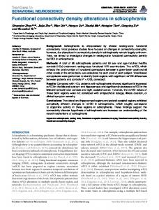
Figure 1. Three-dimensional view of the brain with the 41 ROIs listed in table 1 in Appendix A. The regions are coloured with respect to their locations in Talairach space (Talairach coordinates as RGB values, except the red region that represents the LIFG in an individual subject, see Appendix A for a more detailed description of how the ROIs were created).

boxcar function weight function r 50

100

150

200

250

300

350

400

450

t/s Figure 2. Example of a weight function r for a single condition. The dashed curve is a boxcar function indicating the presence of the condition, i.e. it is one at each time instant when the condition is present and zero at the others. The solid curve represents the weight function r which was used to compute the weighted correlation cr (cf. equation (4.1)) for the represented condition. See text for further explanations. responses and button presses at the end of each production, exactly as would be done during scanning. We measured and compared reaction times (RTs) in all four conditions both during initial overt production, and then during covert production during training, and later during scanning. We were thus able to ensure that the pattern of RTs was similar across the four conditions during overt versus covert production, providing an indirect index of task performance when there was no overt output. After scanning, subjects were then tested outside the scanner one last time (with new stimuli) during overt production, and performance was recorded. All subjects were able to perform the task, even in the most difficult ‘English sentences’ condition. The experiment was performed on a 3-T whole-body system (Bruker, Germany), equipped with a birdcage radio frequency coil and a head-gradient coil insert designed for echoplanar imaging. Functional images were obtained with a T2*-weighted gradient echo planar imaging sequence (TRZ2.4 s, TEZ30 ms). The 64 ! 64 ! 24 images had a resolution of 3.75 ! 3.75 ! 5 mm. A three-dimensional anatomical image (1 ! 1 ! 1.2 mm) was also acquired for each subject.

3. ROI SELECTION We currently perform our analyses of conditiondependent functional connectivity on a set of Phil. Trans. R. Soc. B (2005)

pre-selected ROI. This facilitates intersubject comparability. In principle, an arbitrary number of regions can be included. The regions can either be chosen individually for each subject (e.g. based on activation maps), or from a list of coordinates of interest in Talairach space. For the language experiment, we selected 41 ROIs, listed in table 1 in Appendix A, and shown in figure 1. The regions included either appeared as activated in the experiment or were mentioned in the related literature. The mean signal time course of the voxels in each region was considered as the representative time course of the respective region. 4. CORRELATION MODULATION One of the motivations behind this approach is to go beyond the usual characterization of an experimental paradigm by activation patterns, and to develop a tool that allows characterization of functional connectivity. More precisely, we are interested in how functional connectivity is modulated by the experimental paradigm within one or several sessions. In our case, the conditions are ‘English sentences’, ‘English words’, ‘French sentences’ and ‘French words’ as described in §2. To assess functional connectivity within a single

Connectivity networks in bilinguals

925

function with the canonical haemodynamic response function, and take the absolute value where the resulting function is negative. We perform this last step because a weight function needs to be non-negative, otherwise this could lead to complex values for the weighted correlation. The values of the weighted correlation span the same range as the values of an ordinary correlation, [K1, 1], and have the same interpretation, but differentially emphasize certain parts of the time course from which the correlation is computed.

10 8 6 activation (t–value) region 2

S. Dodel and others

4 2 0 −2 −4 −6 −8 −10 −10

−5 0 5 activation (t – value) region 1

10

Figure 3. Absence of a simple relation between the consistent CM and the activations of the corresponding regions. All contrasts considered in the experiment are included. Crosses correspond to positive CM and circles to negative CM. The diagonal dashed line shows the diagonal at which the activations of the regions are the same, and the horizontal and vertical dashed lines mark the boundaries between the quadrants. It can be seen that when the t-value is approximately t%1.5 in both regions, the sign of the CM cannot be determined by the activations of the corresponding regions, since the crosses and circles overlap. See text for a discussion.

condition, we compute a weighted correlation between the time courses of every pair of regions from predefined ROIs (cf. §3 for how the set of ROIs was created for the present experiment). The weights model the conditions, and hence are specific to the condition under consideration. For two regions that have the centred and normalized time courses xZ(x1,.,xn)T and yZ( y1,.,yn)T, respectively, we define the weighted correlation as covr ðx; yÞ cr ðx; yÞ :Z pffiffiffiffiffiffiffiffiffiffiffiffiffiffiffiffiffiffiffiffiffiffiffiffiffiffiffiffiffi ; varr ðxÞvarr ðyÞ

(4.1)

(a) Condition-specific networks Computing the weighted correlation of all pairs of regions leaves us with a matrix Cr that contains the condition-specific functional connectivity structure (as measured by weighted correlations). In particular, we can interpret every element in Cr as a link in a network, which we will refer to as a ‘condition-specific network’. The significance of a link in these networks was assessed by a Wilcoxon signed-rank test (see §6), and non-significant links were discarded. So for instance, the ‘condition specific network’ for ‘English sentences’ is the one containing the significant weighted correlations cr of equation (4.1) computed with the time-course of the condition ‘English sentences’ as the weight function r. ‘Condition-specific networks’ are likely to be confounded by artefactual functional connectivity correlations owing to factors that are not of interest here, such as cardiac and respiratory processes. The ‘condition-specific networks’ contained a large number of links (acsnZ5%; corrected; see §6), which were essentially all positive. Qualitatively, and in accord with previous work on functional connectivity, we found a number of anatomically symmetric links (e.g. links from one region to two bilaterally homotopic regions) in these networks. In addition, the ‘condition-specific networks’ for different conditions were very similar, probably because artefactual functional connectivity masked condition-specific differences between the networks.

and

(b) CM networks As mentioned above, the networks based on Cr may contain artefacts, and it therefore seems unreasonable to analyse the matrix Cr directly. Instead, we analyse the variations of functional connectivity from one condition to another. These variations are represented for each pair of regions by correlation modulations (CM) srs, which are obtained by a simple subtraction

varr ðxÞ :Z covr ðx; xÞ;

srs Z cr K cs

where rZ(r1,.,rn)T is the condition-specific weight function. In the simplest case, the weight function r is a boxcar function (‘one’ where the condition is present and ‘zero’ elsewhere, cf. dashed curve in figure 2). With the boxcar as a weight function, the weighted correlation corresponds to the standard sample correlation, taking into account only the parts of the time course where the condition is present. However, weighing with the boxcar function may lead to spurious correlations owing to changes in the signal level from one instantiation of the condition to another. We hence build the weight function r (cf. solid curve in figure 2) by convolving the boxcar

of the weighted correlations from equation (4.1) for conditions modelled by r and s, respectively. In matrix notation, this reads SrsZCrKCs. By subtracting we get rid of the artefactual functional connectivity, provided that the underlying artefact-generating processes are stable across conditions, an assumption which is reasonably justified in most experiments. In §7, we show the matrices Srs of CM for the experiment (cf. §2) as networks, taking only the significant values into account (cf. §6). We call the networks from Srs the ‘CM networks’ (we will refer to them either as ‘consistent CM networks’ or as ‘TOEFL CM

with covr ðx; yÞ :Z

n X

r t xt y t ;

tZ1

Phil. Trans. R. Soc. B (2005)

(4.2)

926

S. Dodel and others Connectivity networks in bilinguals LPUT3 LCPUT LINS1

LPUT2

LPUT1 AC3 AC2 AC1

8

MEDFR2

LINS2

0.3

MEDFR1

LINS3

6

RPUT

LIFG

0.2

RCPUT 4

LPREC1

RPREC2 0.1

LPREC2

RPREC1

SMA

RTMP6

2

0 RTMP5

LTMP1 LTMP2

0

–2 – 0.1

RTMP4 RTMP3

LTMP3

–4 – 0.2

RTMP2

LIPAR1

–6 RTMP1

LIPAR2

RIPAR RSPAR2

LSPAR PRCUN1 PRCUN2

LOCC PC1

PC2

ROCC

– 0.3

–8

RSPAR1

Figure 4. ‘Consistent CM network’ of the main effect of task (contrast ‘sentences’ versus ‘words’ collapsed over both languages). ‘Consistent CM networks’ only show significant links at the acnZ5% corrected level (see §6). Coloured nodes correspond to the t-values (left scale on the colour-bar) of the activation. Empty nodes did not show any significant activation. The colours of the links code the mean value of the CM across the 10 subjects (right scale on the colour-bar). Note that significant links may be observed between regions not detected in the corresponding contrast. See §7.1 for a discussion.

LPUT3 LCPUT LINS1

LPUT2

LPUT1 AC3 AC2 AC1

0.5

MEDFR2

LINS2

MEDFR1

LINS3

0.4

0.1

RPUT

LIFG

RCPUT

LPREC1

RPREC2

LPREC2

RPREC1

SMA

RTMP6

0.3 0.2

0.05

0.1 0 RTMP5

LTMP1 LTMP2

RTMP4

0

– 0.1 – 0.2

– 0.05

RTMP3

LTMP3

– 0.3 RTMP2

LIPAR1

RTMP1

LIPAR2

RIPAR RSPAR2

LSPAR PRCUN1 PRCUN2

LOCC PC1

PC2

ROCC

– 0.4

– 0.1

– 0.5

RSPAR1

Figure 5. Consistent CM network of the main effect of task (contrast ‘English’ versus ‘French’ collapsed over both tasks). For the meaning of link and node values see the caption of figure 4. The results are discussed in §7.2.

networks’ depending on how we assessed significance, see §6). The generality of our approach allows us to analyse functional-connectivity variations owing to arbitrary aspects of an experimental paradigm by modelling them in the weight function. Phil. Trans. R. Soc. B (2005)

(c) Relation to PPI The proposed method differs from PPI (Friston et al. 1997) in the following ways. PPI models activity in a given voxel by means of three additive terms: (i) the direct effect of time-series from the source region,

Connectivity networks in bilinguals LPUT3 LCPUT LINS1

LPUT2

S. Dodel and others

927

LPUT1 AC3 AC2 AC1

2.5

MEDFR2

LINS2

MEDFR1

LINS3

0.15

2

RPUT

LIFG

RCPUT

LPREC1

RPREC2

LPREC2

RPREC1

SMA

RTMP6

1.5

0.1

1 0.05 0.5 0

RTMP5

LTMP1 LTMP2

RTMP4

0

– 0.5 – 0.05 –1

RTMP3

LTMP3

– 1.5 RTMP2

LIPAR1

RTMP1

LIPAR2

RIPAR RSPAR2

LSPAR PRCUN1 PRCUN2

LOCC PC1

PC2

ROCC

– 0.1

–2 – 2.5

– 0.15

RSPAR1

Figure 6. Consistent CM network of the contrast ‘English sentences’ versus ‘French sentences’ in both languages. For the meaning of link and node values see the caption of figure 4.

(ii) the direct effect of the contrast vector, (iii) the interaction of the two. The method proposed here considers the difference of weighted correlations across conditions, which should yield results similar to those obtained by term (iii), but would lead to slightly different residuals. The direct effect from the source region is not modelled because it is related mainly to the correlation between the two regions in question and cancels out in the comparison of two conditions. As for the direct effect of the condition vector, it is difficult to tease apart the direct effect of the experimental paradigm from indirect links arising from brain regions acting as relay stations (cf. §5). However, note that our method can also be applied to the residuals, removing the direct effect of the paradigm. Finally, a crucial difference of our method in comparison to PPI is that our method determines a whole network, whereas PPI considers a single region at a time and gives rise to maps that have a similar interpretation as functional connectivity maps. Apart from differences in the way functional interactions are assessed, a method like PPI would work hence on a single row (or column) of the matrix Srs at a time, whereas our method considers the matrix as a whole. Lastly, in addition, we suggest robust statistics across subjects to assess significant networks.

5. SIMULATIONS AND INTERPRETATION (a) Simulations Here, we address the issue of how activation relates to CM, and compare the CM networks from simulated data with those obtained from real data. We produced surrogate data both by modelling them as autoregressive processes of order 1 with various levels of activation, and by phase shuffling of the real data in the Phil. Trans. R. Soc. B (2005)

Fourier domain, which preserves the overall temporal characteristics (power spectrum) of the real data. Activation can have an impact on CM. It is well known that correlations can either be owing to a common input to two regions, or to direct interaction between the regions. Taking the time courses of the residuals, i.e. removing all activations as modelled by the condition time courses, could reduce the number of possible interpretations of CM. This, however, only holds if the activations are equally well captured by the model for all regions, and at the expense of eliminating correlation variations that are owing to activation by direct interaction of two regions. Hence, in this work, we chose to compute the CM networks on the basis of the full time courses of the real data, and to investigate the relationship between activation and CM with surrogate data in which we systematically varied the parameters related to activation and assessed the resulting CM. We modelled the time courses in two parts, one accounting for activation and the second for the remainder of the signal keeping the total variance fixed. As expected, we found that there is an interaction between activation and CM. This interaction is, however, quite complex even if the signals can be explained completely in terms of activation. The value of the CM depends on both the level of overall activation owing to both conditions and on the relative amount of individual activation in the single conditions. The simulations provide a range of CM values that occur in various scenarios with different levels of overall activation for activated, but otherwise random, autoregressive signals. From the simulations, we would expect CMs of approximately jCMj%0.06 for the data analysed in this paper. However, the CM values found

928

S. Dodel and others Connectivity networks in bilinguals

were up to over five times larger, indicating that processes other than activation are responsible for the CM. See Appendix B for more detail. Figure 3 shows consistent CMs (as defined in §6) versus activations of the corresponding regions for all contrasts considered in the present experiment, confirming that not only the occurrence, but also the sign of a significant CM, is to a large extent independent of the activation of the corresponding regions. In addition, we found that CM networks derived from phase shuffled surrogate data are different from those obtained from real data, hence providing further evidence that such networks could not be obtained from random fluctuations. (b) Interpretation Before presenting the results, we discuss their interpretation and validation from a general point of view. We assume that each experimental condition (e.g. ‘English sentences’) is associated with a functional connectivity network which is typical for this condition. As mentioned above, this network is difficult to identify directly as it may be confounded by artefactual functional connectivity (Dodel et al. 2004). This artefactual connectivity is removed when comparing the connectivity between two conditions.3 Subtracting conditions also implies that the networks common to the two conditions are not visible, akin to the standard comparison of the BOLD activity induced by two conditions. The comparison shows the functional connectivity subnetworks by which the two conditions differ, as measured by the CM in different experimental conditions. The simplest case is to assume that each condition is characterized by a network of positive interactions, which, however, as mentioned above, is often masked. A positive link in the CM network corresponds to a stronger functional interaction during the experimental condition in comparison to the control condition. The interpretation of the sign of the link may depend on the nature of the experimental and control conditions. In our experiment, the conditions can be characterized by ‘task difficulty’ and ‘task inclusion’. Different levels in the experimental factors also involve different levels of effort (‘task difficulty’). For instance, tasks in L1 (French) are likely to be easier than tasks in L2 (English). Similarly, tasks involving sentence production require more effort than tasks involving word production. In addition, some contrasts involve tasks that can be characterized in terms of ‘task inclusion’. For instance, at a macroscopic level, it seems reasonable to assume that networks involved in word production will be subnetworks of those involved in sentence production, since word production is a prerequisite of sentence production. In contrast, tasks differing in the factor ‘language’, such as ‘English sentences’ and ‘French sentences’, may or may not involve different components of a language system, but we do not necessarily expect one system to be a subnetwork of the other. In our contrasts, we always subtracted the easier, and/or the ‘included’ task from the more difficult, and/or the ‘including’ one. A positive link in a condition-dependent network that compares two conditions that differ along both the ‘task Phil. Trans. R. Soc. B (2005)

inclusion’ and ‘task difficulty’ axes can be interpreted as increased functional interaction owing to greater task difficulty. On the other hand, a negative link, indicating greater connectivity during the subtracted, second task, could be interpreted as being owing to a more automated processing in the simpler task. Links in networks of contrasts comparing conditions differing in ‘task difficulty’ but not in terms of ‘task inclusion’, can be interpreted in either way. 6. TESTING LINKS’ SIGNIFICANCE A distinctive feature of our approach is that it uses inter-subject variability to assess significance. This was carried out as described below. For every contrast under consideration, e.g. ‘sentences’ versus ‘words’, and for every subject, we assessed the CM network and identified the consistent (positive or negative) links for all subjects (‘consistent CM networks’). However, from the work of Mechelli et al. (2002), we know that functional connectivity networks are likely to vary across subjects, and therefore, so could the CM networks. Part of this variability, however, may be explained by measurable subject characteristics. For instance, in our case, variability may arise as a consequence of differences in the level of the subjects’ proficiency in English. We therefore quantified subjects’ syntactical proficiency in English using a subtest of the TOEFL, and determined significant correlations between the network link values and the TOEFL scores (TOEFL CM network). (a) Consistent CM networks We used the Wilcoxon signed rank statistic to test for the significance of a link across subjects, and determined the networks composed of the links that were significant at a level of acnZ5% corrected. The Wilcoxon signed rank statistic represents a measure of sign consistency of a set of values at the chosen significance level. According to this test, the CMs were required to have the same sign across all 10 subjects; we therefore refer to these networks as ‘consistent CM networks’. The consistent CM networks shown in this article hence have maximum consistency in terms of the sign of the CM. (b) TOEFL CM networks For the ‘TOEFL CM networks’, we correlated the values of the CM srs (cf. §4, equation (4.2)) across subjects with their scores on the TOEFL, and assessed the significance of the resulting correlations c by a t-test with the t-statistics pffiffiffiffiffiffiffiffiffiffiffiffi c pffiffiffiffiffiffiffiffiffiffiffiffiffi n K 2; 2 1 Kc where n is the number of subjects, after a Fisher’s z-transform 1 C srs 1 log ; 2 1 K srs of the CMs srs. We chose to present these networks at a significance level of atnZ5%, not corrected for multiple comparisons. This corresponds to a threshold jcjZ0.63 for the absolute value of the correlation. This rather low significance level seemed justified since the relationship

Connectivity networks in bilinguals between the CM and the score on the TOEFL cannot be expected to be linear. In the figures, however, we also indicated the links which survived a threshold of atnZ1% (uncorrected) in the t-test, corresponding to a threshold of jcjZ0.77 for the correlation, by using thicker lines. 7. RESULTS AND DISCUSSION In this section, we describe the consistent CM networks for the set of 41 ROIs (see §3) for the main effect of task (contrast ‘sentences’ versus ‘words’) and for the main effect of language (contrast ‘English’ versus ‘French’) In addition, we provide evidence that differences in language proficiency can account for the fact that the consistent CM network for the main effect of language is smaller than that for the main effect of task. (a) Sentences versus words The consistent CM network for the contrast ‘sentences’ versus ‘words’ in figure 4 shows the differences between sentence production and word reading collapsed across languages. Note that the CM for the combined contrast was obtained by subtracting the correlation with the sum of the time courses of all conditions containing the task ‘sentences’ as a weight function from the correlation with the sum of the time courses of all conditions containing the task ‘words’ as a weight function. The most striking result here is the large number of links between the LIFG and many other regions, mostly occipital and contralateral regions. As mentioned in the introduction, the LIFG is the region that is most often found to be activated in brain imaging studies of syntactical processing. More generally, the regions that show links in this analysis include ones previously shown to be involved in syntax and in language production (LIFG, left insula, medial frontal cortex, precentral gyrus, and SMA). Two of the strongest positive links occur between the LIFG and the left and right occipital regions (LOCC and ROCC). This finding suggests that more low-level visual areas and higher level language areas such as the LIFG are more correlated during the sentence production compared with the word reading task. Bokde et al. (2001) found a similar pattern of functional connectivity between activity in the ventral LIFG and the occipital cortex during a semantic task involving words, and suggested that such links may develop during semantic processing when the source of the input to the brain is visual. Similarly, our finding of a strong positive link between LIFG and occipital cortices during the sentence compared with the word condition could reflect an aspect of the functional connectivity mechanisms underlying syntactic processing when the input is visual. The many negative links seen in this contrast could reflect greater correlation between these regions during the control (‘word’) condition compared with the experimental (‘sentence’) condition. Greater functional connectivity across regions during the former condition could suggest that processing during the control condition is more ‘automatized’ than it is Phil. Trans. R. Soc. B (2005)

S. Dodel and others

929

during the experimental condition. Indeed, one would expect word reading to be a more automatic process than constructing sentences from a set of words, this latter task being less natural and less frequently encountered in day-to-day life. The posterior cingulate gyrus (PC2) is adjacent to the superior parietal region, which includes attentional regions, and it has been suggested that it is involved in anticipatory allocation of spatial attention. The negative links between this region and regions previously shown to be activated in reading tasks and related to motor/premotor functions (such as the occipital gyri, the left precentral region, and the SMA) may reflect greater functional connectivity of an anticipatory attentional system with lower level visual areas and motor regions during the word reading compared with the sentence production task. (b) English versus French The ‘consistent CM network’ for the contrast ‘English versus French’ in figure 5 shows the main effect of language, collapsing across tasks. As can be seen, this network contains fewer links than are observed in the previous one reflecting the effect of task. In addition, these links involve a different set of brain regions (e.g. the LIFG is now only linked to three regions). The striking differences between this and the above network provide experimental evidence that validates our method, since at random we would expect the number of links to be roughly the same for all contrasts. A further validation of our method is the fact that the network representing the task by language interaction (not shown) contains almost no links, even though from a mathematical point of view this network is equivalent to a main effect network. The fact that all links in the consistent network for the ‘English versus French’ contrast are negative suggests that there is a stronger correlation between regions during the control, ‘French’ condition. Such a result could be owing to more automatic task performance in the native (French) compared with the second (English) language. The finding of fewer links for the effect of language compared with the effect of task could be owing to individual differences in task-dependent functional connectivity networks, possibly related to individual differences in the level of proficiency in the second language. This interpretation is consistent with studies on the neural basis of bilingualism, suggesting greater intersubject variability in the regions activated in the second compared with the first language (Dehaene et al. 1997). Given that we have a measure of syntactical proficiency for each subject (the TOEFL subset scores), we were able to test these interpretations. The TOEFL subtest scores reflect syntactical proficiency in English, and we can assume that syntactical proficiency is similar across subjects in French, which is their native language. We therefore generated both the ‘consistent’ and the ‘TOEFL CM networks’ for the contrast ‘English sentences’ versus ‘French sentences’. The above interpretation predicts that the consistent CM network for this contrast may not yield many links since the sign of the links may not be consistent across subjects owing to individual

930

S. Dodel and others Connectivity networks in bilinguals LPUT3 LCPUT LINS1

LPUT1 AC3 AC2

LPUT2

AC1

0.2

MEDFR2

LINS2

MEDFR1

LINS3

0.15

RPUT

LIFG

1.0 0.8 0.6

RCPUT 0.1

LPREC1

RPREC2

LPREC2

RPREC1

SMA

RTMP6

0.4 0.05

0 RTMP5

LTMP1

– 0.05

LTMP2

RTMP4 RTMP3

LTMP3

0.2 0 – 0.2 – 0.4

– 0.1 – 0.6

RTMP2

LIPAR1

– 0.15

RTMP1

LIPAR2

RIPAR RSPAR2

LSPAR PRCUN1 PRCUN2

LOCC PC1

ROCC

PC2

– 0.2

– 0.8

– 1.0

RSPAR1

Figure 7. ‘TOEFL CM network’ of the contrast ‘English sentences’ versus ‘French sentences’. Only significant links are shown for the correlation between the CM values (srs, cf. §4) and the TOEFL scores (atnZ5% uncorrected), and their value is indicated on the right scale on the colour-bar. Links with thicker lines have a higher significance level (atnZ1% uncorrected). Coloured nodes correspond to the t-values (left scale on the colour-bar) of the correlation between activation and the TOEFL scores. Empty nodes did not show any significant correlation. See §7.2 for a discussion.

interhemispheric links

left intrahemispheric links 60

RPREC1

40 20 0 – 20

AC1

RSPAR1 LSPAR PC1 RPREC2 LPREC1 LINS3 PRCUN2 RTMP4 LIFG LPUT2 LTMP2 RTMP5 LPUT3 RTMP1 RTMP6 ROCC LINS2 RPUT LPUT1 LOCC RCPUT RTMP3

– 40 60 40 20

0 – 20 – 40 – 60 – 80 – 100

60 LSPAR

PC1

40 LPREC1

right intrahemispheric links

RPREC1 RSPAR1

RPREC2 LINS3 PRCUN2 RTMP4 20 LTMP2LIFG LPUT2 RTMP5 LPUT3 RTMP1 LINS2 RPUTROCC RTMP6 LPUT1 0 LOCC AC1 RCPUT RTMP3

– 20

– 40 – 60 – 40 – 20 0

20 40 60

60

RPREC1 RSPAR1 LSPAR

PC1 40 RPREC2 LPREC1 LINS3 PRCUN2 RTMP4 LIFG 20 LTMP2 LPUT2 RTMP5 LPUT3 RTMP1 RTMP6 ROCC LINS2 RPUT LPUT1 0 LOCC RTMP3 RCPUT

AC1

– 20

– 40 –100 –80 –60 –40 – 20 0

20 40 60

all links 60

0.8

AC1

0.6

40 20

0.4

LINS3 LINS2 LIFG

0 LPREC1 LTMP2

RCPUT LPUT3 RPUT LPUT2 LPUT1

– 20

0.2 RTMP1 RTMP3 RTMP4 RPREC1 RPREC2RTMP6

0

PC1

– 40 – 60 – 80

RTMP5 LSPAR

RSPAR1 PRCUN2

LOCC – 100 – 60 – 40 –20

– 0.2 – 0.4 – 0.6

ROCC

– 0.8 0

20 40 60

Figure 8. Network of figure 7 displayed in anatomical projections. Top: Left intrahemispheric links (sagittal view), inter hemispheric links (coronal view), right intrahemispheric links (sagittal view). Bottom: View of the whole network from above.

differences. In contrast, we predict that the ‘TOEFL CM network’ will include regions thought to be involved in syntax, or whose activation is thought to be related to attention and/or task difficulty. Phil. Trans. R. Soc. B (2005)

(i) English sentences versus French sentences In line with the predictions made above, we find the ‘consistent CM network’ for English versus French sentences, shown in figure 6, to be very sparse, whereas

Connectivity networks in bilinguals the TOEFL CM network for this same contrast, shown in figures 7 and 8, exhibits a large number of links. This provides evidence that the inter-subject variability in the processing of L2 versus L1 is at least in part explainable by differences in L2 proficiency. In addition, the fact that most of the links involve theoretically-relevant brain regions further validates our technique. The TOEFL CM network shows mostly positive links between a number of regions that have previously been shown to be involved in syntax and in language production. These include the LIFG (often including Broca’s area), the left and right putamina, the left insula, the left precentral gyrus, and the SMA. We also see positive links in regions involved in the allocation of attention and in response planning, such as the right and left superior parietal lobes and the precuneus. As mentioned above, the LIFG is the brain area most often found to be activated in brain imaging studies of syntactical processing. The positive links between the LIFG and regions that may be involved in sentence production suggest differential modulation between these regions as a function of proficiency in L2. Specifically, the results suggest that in more proficient bilinguals there exists a functional connectivity network that is less present in less proficient bilinguals during sentence production in L2.

8. CONCLUSIONS AND FURTHER DIRECTIONS In this article, we presented a novel approach to functional connectivity which extends PPI (Friston et al. 1997). Our method allows identification of networks of CM for an arbitrary number of regions and analysis of condition-dependent functional interactions within one session. Furthermore, we do not only consider functional connectivity with respect to a single region as is done in seed voxel approaches, but our approach gives rise to a whole network structure which, in contrast to most effective connectivity studies, is not chosen in an a priori manner, but emerges as a result of the analyses. To our knowledge, this is the first presentation of condition-dependent functional interaction within fMRI that includes a large number of regions and that investigates the structure of their functional connectivity as a whole. An additional aspect consists of the assessment of networks in which inter-subject variability of the condition-dependent functional interactions can be explained by a subject-dependent variable, in our case a TOEFL subtest score. Our approach is related to conventional activation analyses in that it uses a priori information from the experimental paradigm. It hence has similar drawbacks, but offers similar advantages as well, particularly in terms of allowing testable hypotheses to be put forth and in terms of result interpretability. Furthermore, our approach operates on a network level, i.e. it emphasizes interactions between regions, which seems appropriate when studying brain function. In contrast to successively determining PPIs for various regions, the network level approach prospectively allows the use of powerful tools from graph theory to Phil. Trans. R. Soc. B (2005)

S. Dodel and others

931

analyse the structure of functional connectivity modulations as a whole. In this paper, we gave a qualitative description of functional connectivity modulation, or CM networks, applied to an experiment on syntax in bilinguals. The results provide a first validation of our method in that the observed network structures are highly unlikely to be owing to random correlation fluctuations, and in that the results are interpretable in terms of previous functional imaging studies. However, further work has to be carried out on automated quantitative characterizations of the networks, and also in terms of including more regions. This latter point can be addressed, for instance, by partitioning the whole brain into non-overlapping, labelled (identified) ROI, which would help to maintain result interpretability. With additional experimental validations of our approach, we hope to further contribute to the notion of large-scale networks in functional brain imaging. The authors are grateful for funding from French Ministry of Research ACI 0066 (Computational Neurosciences: Neurosciences computationnelles et integratives) ACI 0044 (Large data: Masse de Donnees) and ACI Connectivity. NG was partly funded from the ACI plasticite´ ce´re´brale et acquisition du langage.

APPENDIX A: THE 41 ROIS We identified the LIFG for each subject individually as the union of the voxels in the activation maps for ‘English’ versus ‘silence’ and ‘French’ versus ‘silence’. The other regions were created from a list of Talairach coordinates. The ROIs were created by taking spheres with radii of 12 mm around the listed coordinates (the radii of the spheres were 8 mm for the right putamen (RPUT), left insula (LINS2) and right temporal (RTMP2) regions). A voronoi tesselation with the centres of the spheres was then performed to avoid any overlap between the regions. In cases where two or more coordinates of interest were neighbours in a three-dimensional voxel neighbourhood and had identical names associated with them, the coordinates were averaged prior to the voronoi tesselation. Region names still occurring more than once were assigned an index number to distinguish them. The ROIs so obtained were then superimposed on the individual masks for the LIFG, resulting in an individual mask image for each subject. The names of the ROIs considered in this article and their corresponding abbreviations are listed in table 1, together with the sizes of the regions (number of voxels they comprise) and Talairach coordinates of their centre (used for the voronoi tesselation). Region selection facilitates intersubject comparability. However, unless regions are defined for each subject individually, there is a trade-off between the size of a region and the representativeness of its time course. In general, the larger a region, the less representative is its time course, owing to greater variability in the voxel time courses. On the other hand, the smaller a region, the higher the risk that it does not comprise the same structures in all subjects owing to intersubject variability. The choice of our regions seems to represent a reasonable compromise

932

S. Dodel and others Connectivity networks in bilinguals

Table 1. The 41 ROIs constituting the nodes of the networks shown in this article. number

size (in voxels)

coordinates

1 2 3 4 5 6 7 8 9 10 11 12 13 14 15 16 17 18 19 20 21 22 23 24 25 26 27 28 29 30 31 32 33 34 35 36 37 38 39 40 41

83 K4 117 0 117 8 108 K8 individual masks 88 K32 34 K28 123 K28 108 K52 98 K52 123 K28 111 K56 125 K56 71 K24 92 K20 99 K8 120 K36 110 K48 93 K64 84 K60 116 4 123 K28 121 4 115 12 93 K16 73 K12 115 12 174 56 123 32 122 48 116 40 38 16 155 28 106 28 91 44 43 48 90 48 106 48 110 56 100 60 200 K12

52 24 40 12

K4 16 20 K8

K4 16 16 K36 K40 K88 K4 K4 K8 K4 4 K52 K16 K8 K8 52 56 K28 K44 K60 K64 12 K60 K84 K16 K20 0 K56 K52 K16 K32 K16 K16 K40 K20 8

0 4 28 52 40 0 36 48 4 12 4 48 K4 12 4 K4 8 44 32 24 24 K8 32 4 56 36 4 48 36 4 0 K8 20 8 4 60

in this respect, since the results remained stable against changes in the definition of the regions (results not shown here).

APPENDIX B: INTERACTION BETWEEN ACTIVATION AND CM In this section, we show the results of simulating CM networks with surrogate data, addressing the issue of how CM is influenced by brain activation. From the results below, it can be shown that the CM networks observed indicate that processes other than activation are responsible for the CM. Let us consider a region that has the normalized and centred signal x. Further, let the two condition vectors be a and b, respectively, and let 3 be the part of the signal that is not explained by the conditions. A condition vector, a or b, thereby consists in a function (e.g. a boxcar function) modelling the Phil. Trans. R. Soc. B (2005)

name

abbreviation

anterior cingulate cortex anterior cingulate cortex anterior cingulate cortex left caudate nucleus/putamen left inferior frontal gyrus left insula left insula left insula left inferior parietal gyrus left inferior parietal gyrus left occipital cortex left occipital cortex left precentral gyrus left putamen left putamen left putamen left superior parietal gyrus left temporal cortex/Heschls gyrus left temporal cortex left superior temporal gyrus medial frontal cortex medial frontal cortex posterior cingulate cortex posterior cingulate cortex precuneus/posterior cingulate cortex precuneus right caudate nucleus/putamen right inferior parietal gyrus right occipital cortex right precentral gyrus right medial precentral region right putamen right superior parietal gyrus right superior parietal gyrus right temporal cortex right superior temporal gyrus right temporal cortex right temporal cortex right temporal cortex right superior temporal gyrus superior frontal region/supplementary motor area

AC1 AC2 AC3 LCPUT LIFG LINS1 LINS2 LINS3 LIPAR1 LIPAR2 LOCC LPREC1 LPREC2 LPUT1 LPUT2 LPUT3 LSPAR LTMP1 LTMP2 LTMP3 MEDFR1 MEDFR2 PC1 PC2 PRCUN1 PRCUN2 RCPUT RIPAR ROCC RPREC1 RPREC2 RPUT RSPAR1 RSPAR2 RTMP1 RTMP2 RTMP3 RTMP4 RTMP5 RTMP6 SMA

presence and absence of the respective condition. Note that for simplicity we refer to the conditions by their respective condition vectors, a and b. If we assume a, b and 3 to be mutually orthogonal and normalized we can write pffiffiffiffiffiffiffiffiffiffiffiffiffiffiffiffiffiffiffiffiffiffiffiffiffi (A 1) x Z aa C bb C 1 K a2 K b2 3: pffiffiffiffiffiffiffiffiffiffiffiffiffiffiffiffiffiffiffiffiffiffiffiffi The factor gZ 1K a2 K b2 assures the normalization, i.e. the fixed variance of the signal x, independently of the values a and b. The values a and b are referred to in this context as ‘activations’ owing to the conditions a and b, respectively. The term ‘deactivation’ refers to negative a or b. We call ‘overall activation’ the amount of variance owing to both time courses a and b. The overall activation writes s2Za2Cb2. The value g2 corresponds to the variance of the signal x that is not explained by activation. For gZ0 and gZ1, we have two extreme cases where

Connectivity networks in bilinguals

1.0 0.8 0.6 0.4 0.2 0 -0.2 -0.4 -0.6 -0.8 -1.0 -1.0 -0.5

(b)

0 ax

0.5

1.0

-0.15 -0.10 -0.05

0.02 0 -0.01

0 CM

0.05 0.10

(d) 0.10

0.01

ay

(c) 0.20 0.15 0.10 0.05 0 -0.05 -0.10 -0.15 -0.20 -0.2 -0.1

933

0.8 0.6 0.4 0.2 0 -0.2 -0.4 -0.6 -0.8

ay

ay

(a)

S. Dodel and others

0.2 0 -0.2

0.05 0 -0.5

-0.02

0 ax

0.5

-0.05 -0.10

0 0.1 0.2 ax

Figure 9. CMs of two regions with signals x and y for different levels of overall activation for the contrast a versus b. (a) Level of overall activation: s2Z100% in both regions, i.e. the signals x and y are completely determined by the activations in the conditions a and b. ax and ay denote the activations of the respective regions in condition a. The respective activations bx, by in condition b are determined by ax, ay and the fixed level of overall activation s2 by b2Zs2Ka2 (see text). The CMs are strongly dependent on the activations ax and ay in condition a. As expected, the CMs are negative if an activation of a in one region coincides with a deactivation in the other. In contrast, activations of a with the same sign in both regions have a smaller effect on the CMs. If both regions are equally active (axZay and bxZby), the signals are identical and CMZ0. (b) Level of overall activation: s2Z0% (none of the regions is active). CM histogram. Ninety-five percent of the CMs have values of jCMj%0.06, indicated by the two vertical lines. (c) Level of overall activation: s2Z5% in both regions. The CM pattern shown is the mean of several CM patterns for various sample time courses all with s2Z5%. The mean represents well the shape of the CM patterns, however, the magnitude of the patterns may vary from one simulation to the other (and may be all positive in some cases). (d) Level of overall activation: s2x Z 95% in one region and s2y Z 5% in the other. As in (c), the CM pattern shown is the mean of several simulations using sample time courses with the indicated respective overall activations. As can be seen, the pattern represents a mixture of the cases shown in the subfigures (a) and (c).

† the signal x is completely determined by the activations in the conditions a and b. † the region is not active at all in the conditions a and b, i.e. xh3. For a given level of overall activation s2 in the signal time course x, the proportion of activation in the two conditions a and b may still vary. More precisely, for b2Zs2Ka2 the overall activation s2 remains the same whatever the value of a. Figure 9 shows the CM’s of two regions with signals x and y for the contrast a versus b for different levels of overall activation. The signals x and y are modelled by an autoregressive model (of order 1). What can be seen from figure 9 is that, as expected, there is an interaction between activation and CM. However, this interaction is quite complex, even if the signals of the two regions can be completely accounted for by activation (figure 9a). In theory, many different combinations of activations can give rise to the same CM value. Furthermore, figure 9 provides a range of CM values that occur in various scenarios with different levels of overall activation for activated, but otherwise random, autoregressive signals. In the data analysed in the present paper, the mean overall activation of the regions was approximately s 2Z6%, which corresponds approximately to the case shown in figure 9c. From the simulations, we would expect Phil. Trans. R. Soc. B (2005)

CMs of approximately jCMj%0.06, in this case for random signals; however, the CM values we found were up to over five times larger, indicating that processes other than activation are responsible for the CM. ENDNOTES 1

Steady-state functional connectivity should not be confused with resting-state connectivity. Resting-state connectivity is a special case of steady-state connectivity in which the steady-state is ‘rest’. In addition to the shortcomings of steady-state correlations, restingstate studies are even less interpretable, because there is no explicit control over the context in which fluctuations around the steady-state are expressed. 2 This assumes that the artefacts are similar in the various experimental conditions. 3 The physiological artefacts and other confounds can generally be assumed to be independent of experimental conditions.

REFERENCES Abutalebi, J., Cappa, S. F. & Perani, D. 2001 The bilingual brain as revealed by functional neuroimaging. Bilingualism Lang. Cogn. 4, 179–190. Bartlett, E., Brown, J., Wolf, A. & Brodie, J. 1987 Correlations between glucose metabolic rates in brain regions of healthy male adults at rest and during language stimulation. Brain Lang. 32, 1–18. Biswal, B., Yetkin, F., Haughton, V. & Hyde, J. 1995 Functional connectivity in the motor cortex of resting

934

S. Dodel and others Connectivity networks in bilinguals

human brain using echo-planar MRI. Magn. Reson. Med. 34, 537–541. Biswal, B., Van Kylen, J. & Hyde, J. 1997 Simultaneous assessment of flow and bold signals in resting-state functional connectivity maps. NMR Biomed. 10, 165–170. Bokde, A., Tagamets, M., Friedman, R. & Horwitz, B. 2001 Functional interactions of the inferior frontal cortex during the processing of words and word-like stimuli. Neuron 30, 609–617. Bu¨chel, C. & Friston, K. 1997 Modulation of connectivity in visual pathways by attention: cortical interactions evaluated with structural equation modelling and fMRI. Cereb. Cortex 7, 768–778. Bu¨chel, C. & Friston, K. 1998 Dynamic changes in effective connectivity characterized by variable parameter regression and kalman filtering. Hum. Brain Mapp. 6, 403–408. Bullmore, E., Harrison, L., Lee, L., Mechelli, A. & Friston, K. 2004 Brain connectivity workshop, Cambridge UK, May 2003. Neuroinformatics 2, 123–126. Caplan, D., Alpert, N. & Waters, G. 1998 Effects of syntactic structure and propositional number on patterns of regional cerebral blood flow. J. Cogn. Neurosci. 10, 541–552. Chee, M., Caplan, D., Soon, C., Sriram, N., Tan, E., Thiel, T. & Weekes, B. 1999a Processing of visually presented sentences in Mandarin and English studied with fMRI. Neuron 23, 127–137. Chee, M., Tan, E. & Thiel, T. 1999b Mandarin and English single word processing studied with functional magnetic resonance imaging. J. Neurosci. 19, 3050–3056. Cooke A. et al. 2002 Neural basis for sentence comprehension: grammatical and short-term memory components. Hum. Brain Mapp. 15, 80–94. Cordes, P. 2002 Hierarchical clustering to measure connectivity in fMRI resting-state data. Magn. Reson. Imaging 20, 305–317. Cordes, D., Haughton, V. M., Arfanakis, K., Wendt, G. J., Turski, P. A., Moritz, C. H., Quigley, M. A. & Meyerand, M. E. 2000 Mapping functionally related regions of brain with functional connectivity MR imaging. Am. J. Neuroradiol. 21, 1636–1644. Dapretto, M. & Bookheimer, S. Y. 1999 Form and content: dissociating syntax and semantics in sentence comprehension. Neuron 24, 427–432. Dehaene, S., Dupoux, E., Mehler, J., Cohen, L., Paulesu, E., Perani, D., van de Moortele, P.-F., Le´hericy, S. & LeBihan, D. 1997 Anatomical variability in the cortical representation of first and second languages. NeuroReport 8, 3809–3815. Dodel, S., Herrmann, J. M. & Geisel, T. 2002 Functional connectivity by cross-correlation clustering. Neurocomputing 44–46, 1065–1070. Dodel, S., Poline, J.-B., Anton, J.-L. & Brett, M. 2004 The influence of heart beat and respiration on functional connectivity networks. In Proc. 2th Proc. IEEE ISBI, Arlington, VA, pp. 380–383. Embick, D., Marantz, A., Miyashita, Y., O’Neil, W. & Sakai, K. L. 2000 A syntactic specialization for Broca’s area. Proc. Natl Acad. Sci. USA 97, 6150–6154. Fiebach, C., Schlesewsky, M. & Friederici, A. 2001 Syntactic working memory and the establishment of filler-gap dependencies: insights from ERPs and fMRI. J. Psycholinguist. Res. 30, 321–338. Fodor, J. 1999 Let your brain alone. London review of books. Friederici, A. D., Meyer, M. & von Cramon, D. Y. 2000 Auditory language comprehension: an event-related fMRI study on the processing of syntactic and lexical information. Brain Lang. 74, 289–300. Phil. Trans. R. Soc. B (2005)

Friston, K. 1994 Functional and effective connectivity in neuroimaging: a synthesis. Hum. Brain Mapp. 2, 56–78. Friston, K., Frith, C., Liddle, P. & Frackowiak, R. 1993 Functional connectivity: the principal-component analysis of large (PET) data sets. J. Cereb. Blood Flow Metab. 13, 5–14. Friston, K., Buechel, C., Fink, G., Morris, J., Rolls, E. & Dolan, R. 1997 Psychophysiological and modulatory interactions in neuroimaging. NeuroImage 6, 218–229. Friston, K., Harrisson, L. & Penny, W. 2002 Beyond phrenology: what can neuroimaging tell us about distributed circuitry? Annu. Rev. Neurosci. 25, 221–250. Friston, K., Harrison, L. & Penny, W. 2003 Dynamic causal modelling. NeuroImage 19, 1273–1302. Golay, X., Kollias, S., Stoll, G., Meier, D., Valavanis, A. & Boesiger, P. 1998 A new correlation-based fuzzy logic clustering algorithm for fMRI. Magn. Reson. Med. 40, 249–260. Goutte, C., Toft, P., Rostrup, E., Nielsen, F. & Hansen, L. 1999 On clustering fMRI time series. NeuroImage 9, 298–310. Grafton, S., Sutton, J., Couldwell, W., Lew, M. & Waters, C. 1994 Network analysis of motor system connectivity in Parkinson disease: modulation of talamocortical interactions after pallidoctomy. Hum. Brain Mapp. 2, 45–55. Hampson, M., Peterson, B., Skudlarski, P., Gatenby, J. & Gore, J. 2002 Detection of functional connectivity using temporal correlations in MR images. Hum. Brain Mapp. 15, 247–262. He, A., Tan, L., Tang, Y., James, G., Wright, P., Eckert, M., Fox, P. & Liu, Y. 2003 Modulation of neural connectivity during tongue movement and reading. Hum. Brain Mapp. 18, 222–232. Horwitz, B. 2003 The elusive concept of brain connectivity. NeuroImage 19(2 Pt 1), 466–470. Horwitz, B. & Braun, A. 2004 Brain network interactions in auditory, visual and linguistic processing. Brain Lang. 89, 377–384. Horwitz, B., Duara, R. & Rapoport, S. 1984 Intercorrelations of glucose metabolic rates between brain regions: application to healthy males in a state of reduced sensory input. J. Cereb. Blood Flow Metab. 4, 484–499. Horwitz, B., Rumsey, J. & Donohue, B. 1998 Functional connectivity of the angular gyrus in normal reading and dyslexia. Proc. Natl Acad. Sci. 95, 8939–8944. Just, M. A., Carpenter, P. A., Keller, T. A., Eddy, W. F. & Thulborn, K. R. 1996 Brain activation modulated by sentence comprehension. Science 274, 114–116. Just, M., Newman, S., Keller, T., McEleney, A. & Carpenter, P. 2004 Imagery in sentence comprehension: an fMRI study. NeuroImage 21, 112–124. Keller, T., Carpenter, P. & Just, M. 2001 The neural bases of sentence comprehension: a fMRI examination of syntactic and lexical processing. Cereb. Cortex 11, 223–237. Kim, K. H. S., Relkin, N. R., Lee, K.-M. & Hirsch, J. 1997 Distinct cortical areas associated with native and second languages. Nature 388, 171–174. Klein, D., Zatorre, R., Milner, B., Meyer, E. & Evans, A. 1994 Left putaminal activation when speaking a second language: evidence from PET. NeuroReport 5, 2295–2297. Klein, D., Milner, B., Zatorre, R., Meyer, R. & Evans, A. 1995 The neural substrates underlying word generation: a bilingual functional-imaging study. Proc. Natl Acad. Sci. USA 92, 2899–2903. Lahaye, P.-J., Poline, J.-B., Flandin, G., Dodel, S. & Garnero, L. 2003 Functional connectivity: studying non-linear, asynchronous interactions between bold signal. NeuroImage 20, 962–974.

Connectivity networks in bilinguals LeBihan, D. 2003 Looking into the functional architecture of the brain with diffusion MRI. Nat. Rev. Neurosci. 4, 469–480. Lohmann, G. & von Cramon, D. 2001 Detecting functionally coherent networks in fMRI data of the human brain using replicator dynamics. IPMI, pp. 218–224 McIntosh, A. & Gonzalez-Lima, F. 1994 Structural equation modeling and its application to network analysis in functional brain imaging. Hum. Brain Mapp. 2, 2–22. McIntosh, A. & Gonzalez-Lima, F. 1995 Functional network interactions between parallel auditory pathways during pavlovian conditioned inhibition. Brain Res. 683, 228–241. McKeown, M., Jung, T., Makeig, S., Brown, G., Kindermann, S., Lee, T. & Sejnowski, T. 1998 Spatially independent activity patterns in functional MRI data during the stroop color-naming task. Proc. Natl Acad. Sci. 95, 803–810. Mechelli, A., Penny, W., Price, C., Gitelman, D. & Friston, K. 2002 Effective connectivity and intersubject variability: using a multisubject network to test differences and commonalities. NeuroImage 17, 1459–1469. Metter, E., Riege, W., Hanson, W., Camras, L., Phelps, M. & Kuhl, D. 1984 Correlations of glucose metabolism and structural damage to language function in aphasia. Brain Lang. 21, 187–207. Muller, H., Kraft, E., Ludolph, A. & Erne, S. 2002 New methods in fMRI analysis. Hierarchical cluster analysis for improved signal-to-noise ratio compared to standard techniques. IEEE Eng. Med. Biol. Mag. 21, 134–142.

Phil. Trans. R. Soc. B (2005)

S. Dodel and others

935

Ni, W., Constable, R. T., Mencl, W. E., Pugh, K. R., Fulbright, R. K., Shaywitz, S. E., Shaywitz, B. A., Gore, J. C. & Shankweiler, D. 2000 An event-related neuroimaging study distinguishing form and content in sentence processing. J. Cogn. Neurosci. 12, 120–133. Peltier, S. J., Polk, T. A. & Noll, D. C. 2003 Detecting lowfrequency functional connectivity in fMRI using a selforganizing map (SOM) algorithm. Hum. Brain Mapp. 20, 220–226. Penny, W., Stephan, K., Mechelli, A. & Friston, K. 2004 Comparing dynamic causal models. NeuroImage 22, 1157–1172. Perani, D., Paulesu, E., Sebastian, N., Dupoux, E., Dehaene, S., Bettinardi, V., Cappa, S. F., Fazio, F. & Mehler, J. 1998 The bilingual brain: profiency and age of acquisition of the second language. Brain 121, 1841–1852. Sakai, K. L., Noguchi, Y., Takeuchi, T. & Watanabe, E. 2002 Selective priming of syntactic processing by event-related transcranial magnetic stimulation of broca’s area. Neuron 35, 1177–1182. Sun, F., Miller, L. & D’Esposito, M. 2004 Measuring interregional functional connectivity using coherence and partial coherence analyses of fMRI data. NeuroImage 21, 647–658. Tononi, G., McIntosh, A., Russell, D. & Edelman, G. 1998 Functional clustering: identifying strongly interactive brain regions in neuroimaging data. NeuroImage 7, 133–149. Waites, A., Stanislavsky, A., Abbott, D. & Jackson, G. 2004 Effect of prior cognitive state on resting state networks measured with functional connectivity. Hum. Brain Mapp. 24, 59–60.