Tutorials in Quantitative Methods for Psychology 2013, Vol. 9(2), p. 43-60.
Conducting Simulation Studies in the R Programming Environment
Kevin A. Hallgren University of New Mexico
Simulation studies allow researchers to answer specific questions about data analysis, statistical power, and best-practices for obtaining accurate results in empirical research. Despite the benefits that simulation research can provide, many researchers are unfamiliar with available tools for conducting their own simulation studies. The use of simulation studies need not be restricted to researchers with advanced skills in statistics and computer programming, and such methods can be implemented by researchers with a variety of abilities and interests. The present paper provides an introduction to methods used for running simulation studies using the R statistical programming environment and is written for individuals with minimal experience running simulation studies or using R. The paper describes the rationale and benefits of using simulations and introduces R functions relevant for many simulation studies. Three examples illustrate different applications for simulation studies, including (a) the use of simulations to answer a novel question about statistical analysis, (b) the use of simulations to estimate statistical power, and (c) the use of simulations to obtain confidence intervals of parameter estimates through bootstrapping. Results and fully annotated syntax from these examples are provided.
*
Simulations provide a powerful technique for answering a broad set of methodological and theoretical questions and provide a flexible framework to answer specific questions relevant to one’s own research. For example, simulations can evaluate the robustness of a statistical procedure under ideal and non-ideal conditions, and can identify strengths (e.g., accuracy of parameter estimates) and weaknesses (e.g., type-I and type-II error rates) of competing approaches for hypothesis testing.
Correspondence concerning this article should be addressed to Kevin Hallgren, Department of Psychology, 1 University of New Mexico, MSC03 2220, Albuquerque, NM 87106. E-mail:
[email protected]. This research was funded by NIAAA grant F31AA021031. The author would like to thank Mandy Owens, Chris McLouth, and Nick Gaspelin for their feedback on previous versions of this manuscript. *
Simulations can be used to estimate the statistical power of many models that cannot be estimated directly through power tables and other classical methods (e.g., mediation analyses, hierarchical linear models, structural equation models, etc.). The procedures used for simulation studies are also at the heart of bootstrapping methods, which use resampling procedures to obtain empirical estimates of sampling distributions, confidence intervals, and p-values when a parameter sampling distribution is non-normal or unknown. The current paper will provide an overview of the procedures involved in designing and implementing basic simulation studies in the R statistical programming environment (R Development Core Team, 2011). The paper will first outline the logic and steps that are included in simulation studies. Then, it will briefly introduce R syntax that helps facilitate the use of simulations. Three examples will be introduced to show the logic and procedures involved in implementing simulation studies, with fully
43
44 annotated R syntax and brief discussions of the results provided. The examples will target three different uses of simulation studies, including 1. Using simulations to answer a novel statistical question 2. Using simulations to estimate the statistical power of a model 3. Using bootstrapping to obtain a 95% confidence interval of a model parameter estimate For demonstrative purposes, these examples will achieve their respective goals within the context of mediation models. Specifically, Example 1 will answer a novel statistical question about mediation model specification, Example 2 will estimate the statistical power of a mediation model, and Example 3 will bootstrap confidence intervals for testing the significance of an indirect effect in a mediation model. Despite the specificity of these example applications, the goal of the present paper is to provide the reader with an entry-level understanding of methods for conducting simulation studies in R that can be applied to a variety of statistical models unrelated to mediation analysis. Rationale for Simulation Studies Although many statistical questions can be answered directly through mathematical analysis rather than simulations, the complexity of some statistical questions makes them more easily answered through simulation methods. In these cases, simulations may be used to generate datasets that conform to a set of known properties (e.g., mean, standard deviation, degree of zero-inflation, ceiling effects, etc. are specified by the researcher) and the accuracy of the model-computed parameter estimates may be compared to their specified values to determine how adequately the model performs under the specified conditions. Because several methods may be available for analyzing datasets with these characteristics, the suitability of these different methods could also be tested using simulations to determine if some methods offer greater accuracy than others (e.g., Estabrook, Grimm, & Bowles, 2012; Luh & Guo, 1999). Simulation studies typically are designed according to the following steps to ensure that the simulation study can be informative to the researcher’s question: 1. A set of assumptions about the nature and parameters of a dataset are specified. 2. A dataset is generated according to these assumptions. 3. Statistical analyses of interest are performed on this dataset, and the parameter estimates of interest from these analyses (e.g., model coefficient estimates, fit indices, p-values, etc.) are retained.
4. Steps 2 and 3 are repeated many times with many newly generated datasets (e.g., 1000 datatsets) in order to obtain an empirical distribution of parameter estimates. 5. Often, the assumptions specified in step 1 are modified and steps 2-4 are repeated for datasets generated according to new parameters or assumptions. 6. The obtained distributions of parameter estimates from these simulated datasets are analyzed to evaluate the question of interest. The R Statistical Programming Environment The R statistical programming environment (R Development Core Team, 2011) provides an ideal platform to conduct simulation studies. R includes the ability to fit a variety of statistical models natively, includes sophisticated procedures for data plotting, and has over 3000 add-on packages that allow for additional modeling and plotting techniques. R also allows researchers to incorporate features common in most programming languages such as loops, random number generators, conditional (if-then) logic, branching, and reading and writing of data, all of which facilitate the generation and analysis of data over many repetitions that is required for many simulation studies. R also is free, open source, and may be run across a variety of operating systems. Several existing add-on packages already allow R users to conduct simulation studies, but typically these are designed for running simulations for a specific type of model or application. For example, the simsem package provides functions for simulating structural equation models (Pornprasertmanit, Miller, & Schoemann, 2012), ergm includes functions for simulating social network exponential random graphs (Handcock et al., 2012), mirt allows users to simulate multivariate-normal data for item response theory (Chalmers, 2012), and the simulate function in the native stats package allows users to simulate fitted general linear models and generalized linear models. It should be noted that many simulation studies can be conducted efficiently using these pre-existing functions, and that using the alternative, more general method for running simulation studies described here may not always be necessary. However, the current paper will describe a set of general methods and functions that can be used in a variety of simulation studies, rather than describing the methods for simulating specific types of models already developed in other packages. R Syntax R is syntax-driven, which can create an initial hurdle that
45
Table 1 (part A). Common R commands for simulation studies. Commands for working with vectors Command Description Examples c Combines arguments to make #create vector called a which contains the values 3, 5, 4 vectors a = c(3,5,4) #identical to above, uses X = rnorm(N, 0, 1) > M = a*X + rnorm(N, 0, 1) > Y = cp*X + b*M + rnorm(N, 0, 1) The first line of the syntax above creates a random variable X with a mean of zero and a standard deviation of one for N observations. The second line creates a random variable M that regresses onto X with regression coefficient a and a random error with a mean of zero and standard deviation of one (error variances need not be fixed with a mean of zero and standard deviation of one, and can be specified at any value based on previous research or theoretically-expected values). The third line of syntax creates a random variable Y that regresses onto X and M with regression coefficients cp and b, respectively, with a random error that has a mean of zero and standard deviation of one. It will be shown below that the intercept parameters do not affect the significance of a mediation test, and thus the intercepts were left at zero in the three lines of code above; however, the intercept parameter could be manipulated in a similar manner to a, b, and c’ if desired. Statistical analyses are performed and parameters are retained. Once the random variables X, M, and Y have been generated, the next step is to perform a statistical analysis on the simulated data. In mediation analysis, the Sobel test (MacKinnon et al., 1995; Sobel, 1982) is commonly employed (although, see section below on bootstrapping), which tests the significance of a mediation effect by computing the magnitude of the indirect effect as the product of coefficients a and b (ab) and compares this value to the standard error of ab to obtain a z-like test statistic. Specifically, the Sobel test uses the formula (3) where sa and sb are the standard errors of the estimates for regression coefficients a and b, respectively. The product of coefficients ab reflects the degree to which the effect of X on Y is mediated through variable M, and is contained in the numerator of Equation 3. The standard error of the distribution of ab is in the denominator of Equation 3, and the Sobel statistic obtained in the full equation provides a zlike statistic that tests whether the ab effect is significantly
49 different from zero. Because the Sobel test will be computed many times, making a function to compute the Sobel test provides an efficient way to compute the test repeatedly. Such a function is defined below and called sobel_test. The function takes three arguments, vectors X, M, and Y as the first, second, and third arguments, respectively, and computes regression models for M regressed onto X and Y regressed onto X and M. The coefficients representing a, b, sa, and sb in Equation 3 are extracted by calling coefficients, then a Sobel test is computed and returned. > sobel_test M_X = lm(M ~ X) > Y_XM = lm(Y ~ X + M) > a = coefficients(M_X)[2] > b = coefficients(Y_XM)[3] > stdera = summary(M_X)$coefficients[2,2] > stderb = summary(Y_XM)$coefficients[3,2] > sobelz = a*b / sqrt(b^2*stdera^2 + a^2*stderb^2) > return(sobelz) > } Data are generated and analyzed many times under the same conditions. So far syntax has been provided to generate one set of X, M, and Y variables and to compute a Sobel z-statistic from these variables. These procedures can now be repeated several hundred or thousand times to observe how this model behaves across many samples, which may be accomplished with for loops, as shown below. In the syntax below, the procedure for generating data and computing a Sobel test is repeated reps number of times, where reps is a single integer value. For each iteration of the for loop, data are saved to a matrix called d to retain information about the iteration number (i), a, b, and c’ parameters (a, b, and cp), the sample size (N), an indexing variable that tells whether the test statistic corresponds with an X-M-Y or X-Y-M mediation model (1 vs. 2), and the computed Sobel test statistic which calls on the sobel_test function above. > for (i in 1:reps){ > X = rnorm(N, 0, 1) > M = a*X + rnorm(N, 0, 1) > Y = cp*X + b*M + rnorm(N, 0, 1) > d = rbind(d, c(i, a, b, cp, N, 1, sobel_test(X, M, Y))) > d = rbind(d, c(i, a, b, cp, N, 2, sobel_test(X, Y, M)))
> } The above steps can then be repeated for datasets generated according to different parameters. In the present example, we wish to test three different values of a, b, c’, and N. Syntax for manipulating these parameters is included below. The values selected for a, b, c’, and N are specified as vectors called a_list, b_list, cp_list, and N_list, respectively. Four nested for loops index through each of the values in a_list, b_list, cp_list, and N_list and extract single values for these parameters that are used for data generation. For each combination of a, b, c’, and N, reps number of datasets are generated and subjected to the Sobel test using the same syntax presented above (some syntax is omitted below for brevity, and full syntax with more detailed annotation for this example is provided in Appendix A), and the data are then saved to a matrix called d: > > > > > > > > > > > >
N_list = c(100, 300) a_list = c(-.3, 0, .3) b_list = c(-.3, 0, .3) cp_list = c(-.2, 0, .2) reps = 1000 for (N in N_list){ for (a in a_list){ for (b in b_list){ for (cp in cp_list){ for (i in 1:reps){ X = rnorm(N, 0, 1) M = a*X + rnorm(N, 0, 1) #... syntax omitted > d = rbind(d, c(i, a, b, cp, N, 2, sobel_test(X, Y, M))) > > > > } > }
} } }
Retained parameter estimates are analyzed to evaluate the question of interest. Executing the syntax above generates a matrix d that contains Sobel test statistics for X-M-Y (omitted for brevity) and X-Y-M mediation models (shown above) generated from a variety of a, b, c’, and N parameters. The next step is to evaluate the results of these models. Before this is done, it will be helpful to add labels to the variables in matrix d to allow for easy extraction of subsets of the results and to facilitate their interpretation:
2 1 -1
0
Sobel z-statistic
3
4
5
50
X-M-Y model (a=0.3, b=0.3, c'=0.2)
X-Y-M model (a=0.3, b=0.3, c'=0.2)
X-M-Y model (a=0.3, b=0.3, c'=0)
X-Y-M model (a=0.3, b=0.3, c'=0)
Figure 2. Boxplot of partial results from Example 1 with N = 300.
> colnames(d) = c("iteration", "a", "b", "cp", "N", "model", "Sobel_z") It is also desirable to save a backup copy of the results using the command > write.table(d, "C:\\...\\mediation_output.csv", sep=",", row.names=FALSE) In the syntax above, “...” must be replaced with the directory where results should be saved, and each folder must be separated by double backslashes (“\\”) if the R program is running on a Windows computer (on Macintosh, a colon “:” should be used, and in Linux/Unix, a single forward slash “/” should be used). Researchers can choose any number of ways to analyze the results of simulation studies, and the method chosen should be based on the nature of the question under examination. One way to compare the distributions of Sobel z-statistics obtained for the X-M-Y and X-Y-M mediation models in the current example is to use boxplots, which can be created in R (see ?boxplot for details) or other statistical
software by importing the mediation_output.csv file into other data analytic software. As seen in Figure 2, in the first two conditions where the population parameters a = 0.3, b = 0.3, and c’ = 0.2, Sobel tests for X-M-Y and X-Y-M mediation models produce test statistics with nearly identical distributions and Sobel test-values are almost always significant (|z| > 1.96, which corresponds with p < .05, two-tailed) when N = 300 and other assumptions described above are held. In the latter two conditions where the population parameters a = 0.3, b = 0.3, and c’ = 0, Sobel tests for X-M-Y models remain high, while test statistics for X-Y-M models are lower even though approximately 25% of these models still had Sobel z-test statistics with magnitudes greater than 1.96 (and thus, p-values less than 0.05). The similarity of results between X-M-Y and X-Y-M models suggests limitations of using mediation analysis to identify causal relationships. Specifically, the same datasets may produce significant results under a variety of models that support different theories of the causal ordering of relations. For example, a variable that is truly a mediator may instead be specified as an outcome and still produce “significant” results in a mediation analysis. This could imply misleading support for a causal chain due to the way researchers specify the ordering of variables in the analysis.
51 This finding suggests that mediation analysis may produce misleading results in some situations, particularly when data are cross-sectional because of the lack of temporalordering for observations of X, M, and Y that could provide stronger testing of a proposed causal sequence (Maxwell & Cole, 2007; Maxwell, Cole, & Mitchell, 2011). One implication of these findings is that researchers who perform mediation analysis should test alternative models. For example, researchers could test alternative models with assumed mediators modeled as outcomes and assumed outcomes modeled as mediators to test whether other plausible models are also “significant” (e.g., Witkiewitz et al., 2012).
Example 2: Estimating the Statistical Power of a Model Simulations can be used to estimate the statistical power of a model -- i.e., the likelihood of rejecting the null hypothesis for a particular effect under a given set of conditions. Although statistical power can be estimated directly for many analyses with power tables (e.g., Maxwell & Delaney, 2004) and free software such as G*Power (Erdfelder, Faul, & Buchner, 2006; see Mayr, Erdfelder, Buchner, & Faul, 2007 for a tutorial on using G*Power), many types of analyses currently have no well-established method to directly estimate statistical power, as is the case with mediation analysis. The steps in Example 1 provide the necessary data to estimate the power of a mediation analysis if the assumptions and parameters specified in Example 1 remain the same. Thus, using the simulation results saved in dataset d generated in Example 1, the power of a mediation model under a given set of conditions can be estimated by identifying the relative frequency in which a mediation test was significant. For example, the syntax below extracts the Sobel test statistic from dataset d under the condition where a = 0.3, b = 0.3, c’ = 0.2, N = 300, and “model” = 1 (i.e., an X-M-Y mediation model is tested). The vector of Sobel test statistics across 1000 repetitions is saved in a variable called z_dist. The absolute value each of the numbers in z_dist is compared against 1.96 (i.e., the z-value that corresponds with p < 0.05, two-tailed), creating a vector of values that are either TRUE (if the absolute value is greater than 1.96) or FALSE (if the absolute value is less than or equal to 1.96). The number of TRUE and FALSE values can be summarized using the table command (see ?table for details), which if divided by the length of the number of values in the vector will provide the proportion of Sobel tests with absolute value greater than 1.96:
> z_dist = d$Sobel_z[d$a==0.3 & d$b==0.3 &
d$cp==0.2 & d$N==300 & d$model==1] > significant = abs(z_dist) > 1.96 > table(significant)/length(significant) When the above syntax is run, the following result is printed
significant FALSE TRUE 0.003 0.997 which indicates that 99.7% of the datasets randomly sampled under the conditions specified above produced significant Sobel tests, and that the analysis has an estimated power of 0.997. One could also test the power of mediation models with different parameters specified. For example, the power of a model with all the same parameters as above except with a smaller sample size of N = 100 could be examined using the syntax
> z_dist = d$Sobel_z[d$a==0.3 & d$b==0.3 & d$cp==0.2 & d$N==100 & d$model==1] > significant = abs(z_dist) > 1.96 > table(significant)/length(significant) which produces the following output
significant FALSE TRUE 0.485 0.515 The output above indicates that only 51.5% of the mediation models in this example were significant, which reflects the reduced power rate due to the smaller sample size. Full syntax for this example is provided in Appendix B.
Example 3: Bootstrapping to Obtain Confidence Intervals In the above examples, the Sobel test was used to determine whether a mediation effect was significant. Although the Sobel test is more robust than other methods such as Baron and Kenny’s (1984) causal steps approach (Hayes, 2009; McKinnon et al., 1995), a limitation of the Sobel test is that it assumes that the sampling distribution of indirect effects (ab) is normally distributed in order for the pvalue obtained from the z-like statistic to be valid. This assumption typically is not met because the sampling distributions for a and b are each independently normal, and multiplying a and b introduces skew into the sampling distribution of ab. Bootstrapping can be used as an alternative to the Sobel test to obtain an empirically derived sampling distribution with confidence intervals that are
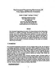
52 more accurate than the Sobel test. To obtain an empirical sampling distribution of indirect effects ab, N randomly selected participants from an observed dataset are sampled with replacement, where N is equal to the original sample size. A dataset containing the observed X, M, and Y values for these randomly resampled participants is created and subject to a mediation analysis using Equations 1 and 2. The a and b coefficients are obtained from these regression models, and the product of these coefficients, ab, is computed and retained. This procedure is repeated many times, perhaps 1000 or 10,000 times, with a new set of subjects from the original sample randomly selected with replacement each time (Hélie, 2006). This provides an empirical sampling distribution of the product of coefficients ab that no longer requires the standard error of the estimate for ab to be computed. The syntax below provides the steps for bootstrapping a 95% confidence interval of an indirect effect for variables X, M, and Y. A variable called ab_vector holds the bootstrapped distribution of ab values, and is initialized using the NULL argument to remove any data previously stored in this variable. A for loop is specified to repeat reps number of times, where reps is a single integer representing the number of repetitions that should be used for bootstrapping. Variable s is a vector containing row numbers of participants that are randomly sampled with replacement from the original observed sample (raw data for X, M, and Y in this example is provided in the supplemental file mediation_raw_data.csv; see Appendix C for syntax to import this dataset into R). The vectors Xs, Ys, and Ms store the values for X, Y, and M, respectively, that correspond with the subjects resampled based on the vector s. Finally, M_Xs and Y_XMs are lm objects containing linear regression models for Ms regressed onto Xs and for Ys regressed onto Xs and Ms, respectively, and the a and b coefficients in these two models are extracted. The product of coefficients ab is computed and saved to ab_vector, then the resampling process and computation of the ab effect are repeated. Once the repetitions are completed, 95% confidence interval limits are obtained using the quantile command to identify the values in ab_vector at the 2.5th and 97.5 percentiles (these values could be adjusted to obtain different confidence intervals; enter ?quantile in the R console for more details), and the result is saved in a vector called bootlim. Finally, a histogram of the ab effects in ab_vector is printed and displayed in Figure 3.
> ab_vector = NULL > for (i in 1:reps){ > s = sample(1:length(X), replace=TRUE)
> Xs = X[s] > Ys = Y[s] > Ms = M[s] > M_Xs = lm(Ms ~ Xs) > Y_XMs = lm(Ys ~ Xs + Ms) > a = M_Xs$coefficients[2] > b = Y_XMs$coefficients[3] > ab = a*b > ab_vector = c(ab_vector, ab) > } > bootlim = c(quantile(ab_vector, 0.025), quantile(ab_vector, 0.975)) > hist(ab_vector) Full syntax with annotation for the bootstrapping procedure above is provided in Appendix C. Calling the bootlim vector returns the indirect effects that correspond with the 2.5th and 97.5th percentile of the empirical sampling distribution of ab, giving the following output:
2.5% 0.06635642
97.5% 0.17234665
Because the 95% confidence interval does not contain zero, the results indicate that the product of coefficients ab is significantly different than zero at p < 0.05.
Discussion The preceding sections provided demonstrations of methods to implement simulation studies for different purposes, including answering novel questions related to statistical modeling, estimating power, and bootstrapping confidence intervals. The demonstrations presented here used mediation analysis as the content area to demonstrate the underlying processes used in simulation studies, but simulation studies are not limited only to questions related to mediation. Virtually any type of analysis or model could be explored using simulation studies. While the way that researchers construct simulations depends largely on the research question of interest, the basic procedures outlined here can be applied to a large array of simulation studies. While it is possible to run simulation studies in other programming environments (e.g., the latent variable modeling software MPlus, see Muthén & Muthén, 2002), R may provide unique advantages to other programs when running simulation studies because it is free, open source, and cross-platform. R also allows researchers to generate and manipulate their data with much more flexibility than many other programs, and contains packages to run a multitude of statistical analyses of interest to social science
53 researchers in a variety of domains. There are several limitations of simulation studies that should be noted. First, real-world data often do not adhere to the assumptions and parameters by which data are
estimates, the exact value for these population parameters is still unknown due to sampling error. To deal with this, researchers can run simulations across a variety of parameter values, as was done in Examples 1 and 2, to
Figure 3. Empirical distribution of indirect effects (ab) used for bootstrapping a confidence interval.
generated in simulation studies. For example, unlike the linear regression models for the examples above, it is often the case in real world studies that residual errors are not homoscedastic and serially uncorrelated. That is, real-world datasets are likely to be more “dirty” than the “clean” datasets that are generated in simulation studies, which are often generated under idealistic conditions. While these “dirty” aspects of data can be incorporated into simulation studies, the degree to which these aspects should be modeled into the data may be unknown and thus at times difficult to incorporate in a realistic manner. Second, it is practically impossible to know the values of true population parameters that are incorporated into simulation studies. For example, in the mediation examples above, the regression coefficients a, b, and c’ often may be unknown for a question of interest. Even if previous research provides empirically-estimated parameter
understand how their models may perform under different conditions, but pinpointing the exact parameter values that apply to their question of interest is unrealistic and typically impossible. Third, simulation studies often require considerable computation time because hundreds or thousands of datasets often must be generated and analyzed. Simulations that are large or use iterative estimation routines (e.g., maximum likelihood) may take hours, days, or even weeks to run, depending on the size of the study. Fourth, not all statistical questions require simulations to obtain meaningful answers. Many statistical questions can be answered through mathematical derivations, and in these cases simulation studies can demonstrate only what was shown already to be true through mathematical proofs (Maxwell & Cole, 1995). Thus, simulation studies are utilized best when they derive answers to problems that do
54 not contain simple mathematical solutions. Simulation methods are relatively straightforward once the assumptions of a model and the parameters to be used for data generation are specified. Researchers who use simulation methods can have tight experimental control over these assumptions and their data, and can test how a model performs under a known set of parameters (whereas with real-world data, the parameters are unknown). Simulation methods are flexible and can be applied to a number of problems to obtain quantitative answers to questions that may not be possible to derive through other approaches. Results from simulation studies can be used to test obtained results with their theoretically-expected values to compare competing approaches for handling data, and the flexibility of simulation studies allows them to be used for a variety of purposes.
References Baron, R. M., & Kenny, D. A. (1986). The moderatormediator distinction in social psychological research: Conceptual, strategic, and statistical considerations. Journal of Personality and Social Psychology, 51(6), 1173– 1182. Chalmers, P. (2012). Multidimensional Item Response Theory [computer software]. Available from http://cran.r-project.org/web/packages/mirt/index.html. Erdfelder, E., Faul, F., & Buchner, A. (1996). GPOWER: A general power analysis program. Behavior Research Methods, Instruments & Computers, 28(1), 1–11. Estabrook, R., Grimm, K. J. & Bowles, R. P. (2012, January 23). A Monte Carlo simulation study assessment of the reliability of within–person variability. Psychology and Aging. Advance online publication. doi: 10.1037/a0026669 Handcock, M. S., Hunder, D. R., Butts, C. T., Goodreau, S. M., Krivitsky, P. N., & Morris, M. (2012). Fit, Simulate, and Diagnose Exponential-Family Models for Networks [computer software]. Available from http://cran.rproject.org/web/packages/ergm/index.html. Hayes, A. F. (2009). Beyond Baron and Kenny: Statistical mediation analysis in the new millennium. Communication Monographs, 76(4), 408-420. Hélie, S. (2006). An introduction to model selection: Tools and algorithms. Tutorials in Quantitative Methods for Psychology, 2(1), 1-10. Jo, B. (2008). Causal inference in randomized experiments with mediational processes. Psychological Methods, 13(4), 314–336. Kabacoff, R. (2012). Quick-R: Accessing the power of R. Retrieved from http://www.statmethods.net/ Luh, W., Guo, J. (1999). A powerful transformation trimmed
mean method for one-way fixed effects ANOVA model under non-normality and inequality of variances. British Journal of Mathematical and Statistical Psychology, 52(2), 303-320. MacKinnon, D. P., Warsi, G., & Dwyer, J. H. (1995). A simulation study of mediated effect measures. Multivariate Behavioral Research, 30, 41-62. Maxwell, S. E., & Cole, D. A. (1995). Tips for writing (and reading) methodological articles. Psychological Bulletin 118(2), 193-198. Maxwell, S. E., Cole, D. A., & Mitchell, M. A. (2011). Bias in cross-sectional analyses of longitudinal mediation: Partial and complete mediation under an autoregressive model. Multivariate Behavioral Research 45, 816-841. Maxwell, S. E., & Delaney, H. D. (2004). Designing experiments and analyzing data: A model comparison perspective (2nd ed.). Mahwah, NJ: Lawrence Erlbaum. Mayr, S., Erdfelder, E., Buchner, A., & Faul, F. (2007). A short tutorial of GPower. Tutorials in Quantitative Methods for Psychology, 3(2), 51–59. Muthén, L. K., & Muthén, B. O. (2002). Teacherʼs corner: How to use a Monte Carlo study to decide on sample size and determine power. Structural Equation Modeling: A Multidisciplinary Journal, 9(4), 599–620. Owen, W. J. (2010). The R guide. Retrieved from http://cran.rproject.org/doc/contrib/Owen-TheRGuide.pdf Pornprasertmanit, S., Miller, P., & Schoemann, A. (2012). SIMulated Structural Equation Modeling [computer http://cran.rsoftware]. Available from project.org/web/packages/simsem/index.html. R Development Core Team (2011). R: A Language and Environment for Statistical Computing [computer software]. Available from http://www.R-project.org Spector, P. (2004). An introduction to R. Retrieved from http://www.stat.berkeley.edu/~spector/R.pdf Sobel, M. E. (1982). Asymptotic intervals for indirect effects in structural equations models. In S. Leinhart (Ed.), Sociological methodology 1982 (pp.290-312). San Francisco: Jossey-Bass. Venables, W. N., Smith, D. M., and the R Development Core Team (2012). An introduction to R. Retrieved from http://cran.r-project.org/doc/manuals/R-intro.pdf
55 Witkiewitz, K., Donovan, D. M., & Hartzler, B. (2012). Drink refusal training as part of a combined behavioral intervention: Effectiveness and mechanisms of change. Journal of Consulting and Clinical Psychology 80(3), 440-449. Manuscript received 12 September 2012 Manuscript accepted 26 November 2012 Appendices follow.
56
Appendix A: Syntax for Example 1
#Answering a novel question about mediation analysis #This simulation will generate mediational datasets with three variables, #X, M, and Y, and will calculate Sobel z-tests for two competing mediation #models in each dataset: the first mediation model proposing that M mediates #the relationship between X and Y (X-M-Y mediation model), the second #mediation model poposes that Y mediates the relationship between X and M #(X-Y-M mediation model). #Note this simulation may take 10-45 minutes to complete, depending on #computer speed #Data characteristics specified by researcher -- edit these as needed N_list = c(100, 300) #Values for N (number of participants in sample) a_list = c(-.3, 0, .3) #values for the "a" effect (regression coefficient #for X->M path) b_list = c(-.3, 0, .3) #values for the "b" effect (regression coefficient #for M->Y path after X is controlled) cp_list = c(-.2, 0, .2) #values for the "c-prime" effect (regression #coefficient for X->Y after M is controlled) reps = 1000 #number of datasets to be generated in each condition #Set starting seed for random number generator, this is not necessary but #allows results to be replicated exactly each time the simulation is run. set.seed(192) #Create a function for estimating Sobel z-test of mediation effects sobel_test 1.96 #identify the proportion of z-values with p-value < 0.05. The proportion of #values that are TRUE is equal to the proportion of times the null hypothesis #of no indirect effect is rejected and is equivalent to power. table(significant)/length(significant) #Other example where a = 0.3, b=0, c'=0.2, N = 300 #extract Sobel z-statistic from the condition of interest z_dist = d$Sobel_z[d$a==0.3 & d$b==0 & d$cp==0.2 & d$N==300 & d$model==1] #identify which z-values are large enough to give p-value < 0.05 significant = abs(z_dist) > 1.96 #identify the proportion of z-values with p-value < 0.05. The proportion of #values that are TRUE is equal to the proportion of times the null hypothesis #of no indirect effect is rejected and is equivalent to power. table(significant)/length(significant)
60
Appendix C: Syntax for Example 3
#Bootstrapping a 95% CI for mediation test #Create a function for bootstrapping mediation_bootstrap M relationship b = Y_XMs$coefficients[3] #extract beta coefficient for #magnitude of M->Y relationship #(with X covaried) ab = a*b #compute product of coefficients ab_vector = c(ab_vector, ab) #save each computed product of #coefficients to vector called #ab_vector } bootlim = c(quantile(ab_vector, 0.025), quantile(ab_vector, 0.975)) #identify ab values at 2.5 and 97.5 percentile, representing 95% #CI hist(ab_vector) segments(bootlim, y0=0, y1=1000, lty=2) text(bootlim, y=1100, labels=c("2.5 %ile", "97.5 %ile")) return(bootlim) #return the 95% CI } #Set starting seed for random number generator, this is not necessary but #allows results to be replicated exactly each time the simulation is run. set.seed(192) #import raw data for bootstrapping (change file path as needed) d_raw = read.csv("C:\\Users\\...\\mediation_raw_data.csv", sep=",")
header=TRUE,
#identify 95% confidence interval for indirect effect in X-M-Y mediation #model mediation_bootstrap(d_raw$X, d_raw$M, d_raw$Y, 1000)