CONNECTIONIST SPEECH RECOGNITION A Hybrid ... - CiteSeerX

CONNECTIONIST SPEECH RECOGNITION A Hybrid Approach by Hervé Bourlard Nelson Morgan

Foreword by Richard Lippmann

KLUWER ACADEMIC PUBLISHERS, ISBN 0-7923-9396-1, 1994

Copyright Page

Contents List of Figures

vii

List of Tables

ix

Notation

xi

Foreword

xv

Preface

xvii

Acknowledgments

xix

I BACKGROUND

1

1 INTRODUCTION 1.1 Automatic Speech Recognition (ASR) . . . . . . . . . . . . . 1.2 Limitations in Current ASR Systems . . . . . . . . . . . . . . 1.3 Book Overview . . . . . . . . . . . . . . . . . . . . . . . . .

3 4 8 9

2 STATISTICAL PATTERN CLASSIFICATION 2.1 Introduction . . . . . . . . . . . . . . . . . 2.2 A Model for Pattern Classification . . . . . 2.3 Statistical Classification . . . . . . . . . . . 2.4 Pattern Classification with Realistic Data . . 2.5 Summary . . . . . . . . . . . . . . . . . .

. . . . .

. . . . .

. . . . .

. . . . .

. . . . .

. . . . .

. . . . .

. . . . .

. . . . .

. . . . .

13 13 14 15 19 21

3 HIDDEN MARKOV MODELS 3.1 Introduction . . . . . . . . . . . . . . . 3.2 Definition and Underlying Hypotheses . 3.3 Parametrization and Estimation . . . . . 3.3.1 General Formulation . . . . . . 3.3.2 Continuous Input Features . . . 3.3.3 Discrete Input Features . . . . . 3.3.4 Maximum Likelihood Criterion

. . . . . . .

. . . . . . .

. . . . . . .

. . . . . . .

. . . . . . .

. . . . . . .

. . . . . . .

. . . . . . .

. . . . . . .

. . . . . . .

23 23 26 28 28 32 33 35

v

. . . . . . .

. . . . . . .

CONTENTS

vi . . . . . . . . .

. . . . . . . . .

. . . . . . . . .

. . . . . . . . .

. . . . . . . . .

. . . . . . . . .

. . . . . . . . .

. . . . . . . . .

. . . . . . . . .

. . . . . . . . .

. . . . . . . . .

36 37 38 40 43 43 44 45 48

4 MULTILAYER PERCEPTRONS 4.1 Introduction . . . . . . . . . . . . . . . . . 4.2 Linear Perceptrons . . . . . . . . . . . . . 4.2.1 Linear Discriminant Function . . . 4.2.2 Least Mean Square Criterion . . . . 4.2.3 Normal Density . . . . . . . . . . . 4.3 Multilayer Perceptrons (MLP) . . . . . . . 4.3.1 Some History . . . . . . . . . . . . 4.3.2 Motivations . . . . . . . . . . . . . 4.3.3 Architecture and Training Procedure 4.3.4 Lagrange Multipliers . . . . . . . . 4.3.5 Speeding up EBP . . . . . . . . . . 4.3.6 On-Line and Off-Line Training . . 4.4 Nonlinear Discrimination . . . . . . . . . . 4.4.1 Nonlinear Functions in MLPs . . . 4.4.2 Phonemic Strings to Words . . . . . 4.4.3 Acoustic Vectors to Words . . . . . 4.5 MSE and Discriminant Distance . . . . . . 4.6 Summary . . . . . . . . . . . . . . . . . .

. . . . . . . . . . . . . . . . . .

. . . . . . . . . . . . . . . . . .

. . . . . . . . . . . . . . . . . .

. . . . . . . . . . . . . . . . . .

. . . . . . . . . . . . . . . . . .

. . . . . . . . . . . . . . . . . .

. . . . . . . . . . . . . . . . . .

. . . . . . . . . . . . . . . . . .

. . . . . . . . . . . . . . . . . .

. . . . . . . . . . . . . . . . . .

51 51 52 52 53 54 55 55 55 57 59 61 62 63 63 65 66 67 68

3.4

3.5

3.6 3.7

3.3.5 Viterbi Criterion . . . . . . . . Training Problem . . . . . . . . . . . . 3.4.1 Maximum Likelihood Criterion 3.4.2 Viterbi Criterion . . . . . . . . Decoding Problem . . . . . . . . . . . 3.5.1 Maximum Likelihood Criterion 3.5.2 Viterbi Criterion . . . . . . . . Likelihood and Discrimination . . . . . Summary . . . . . . . . . . . . . . . .

. . . . . . . . .

II HYBRID HMM/MLP SYSTEMS

69

5 SPEECH RECOGNITION USING ANNs 5.1 Introduction . . . . . . . . . . . . . . . . . . . . . . 5.2 Fallacious Reasons for Using ANNs . . . . . . . . . 5.3 Valid Reasons for Using ANNs . . . . . . . . . . . . 5.4 Neural Nets and Time Sequences . . . . . . . . . . . 5.4.1 Static Networks with Buffered Input . . . . . 5.4.2 Recurrent Networks . . . . . . . . . . . . . 5.4.3 Partial Feedback of Context Units . . . . . . 5.4.4 Approximating Recurrent Networks by MLPs 5.4.5 Discussion . . . . . . . . . . . . . . . . . . 5.5 ANN Models of HMMs . . . . . . . . . . . . . . . .

71 71 72 75 76 77 79 80 82 84 84

. . . . . . . . . .

. . . . . . . . . .

. . . . . . . . . .

. . . . . . . . . .

. . . . . . . . . .

CONTENTS

5.6 5.7

5.5.1 The Viterbi Network . . . . . . . . . . . . . . 5.5.2 The Alpha-Net . . . . . . . . . . . . . . . . . 5.5.3 Combining ANNs and Dynamic Time Warping 5.5.4 ANNs for Nonlinear Transformations . . . . . 5.5.5 ANNs for Preprocessing . . . . . . . . . . . . Discrimination with Contextual MLPs . . . . . . . . . Summary . . . . . . . . . . . . . . . . . . . . . . . .

6 STATISTICAL INFERENCE IN MLPs 6.1 Introduction . . . . . . . . . . . . . . . . . . . . . . . 6.2 ANNs and Statistical Inference . . . . . . . . . . . . . 6.2.1 Discrete Case . . . . . . . . . . . . . . . . . . 6.2.2 Continuous Case . . . . . . . . . . . . . . . . 6.3 Recurrent MLP with Output Feedback . . . . . . . . . 6.4 Practical Implications . . . . . . . . . . . . . . . . . . 6.4.1 Local Minima . . . . . . . . . . . . . . . . . . 6.4.2 Network Outputs Sum to One . . . . . . . . . 6.4.3 Prior Class Probabilities and Likelihoods . . . 6.4.4 Priors and MLP Output Biases . . . . . . . . . 6.4.5 Conclusion . . . . . . . . . . . . . . . . . . . 6.5 MLPs with Contextual Inputs . . . . . . . . . . . . . . 6.6 Classification of Acoustic Vectors . . . . . . . . . . . 6.6.1 Experimental Approach . . . . . . . . . . . . 6.6.2 MLP Approach, Training and Cross-validation 6.6.3 MLP Results . . . . . . . . . . . . . . . . . . 6.6.4 Assessing Bayesian Properties of MLPs . . . . 6.6.5 Effect of Cross-Validation . . . . . . . . . . . 6.6.6 Output Sigmoid Function . . . . . . . . . . . . 6.6.7 Feature Dependence . . . . . . . . . . . . . . 6.7 Radial Basis Functions . . . . . . . . . . . . . . . . . 6.7.1 General Approach . . . . . . . . . . . . . . . 6.7.2 RBFs and Tied Mixtures . . . . . . . . . . . . 6.7.3 RBFs for MAP Estimation . . . . . . . . . . . 6.7.4 Lagrange Multipliers . . . . . . . . . . . . . . 6.7.5 Discussion . . . . . . . . . . . . . . . . . . . 6.8 MLPs for Autoregressive Modeling . . . . . . . . . . 6.8.1 Linear Autoregressive Modeling . . . . . . . . 6.8.2 Predictive Neural Networks . . . . . . . . . . 6.8.3 Statistical Interpretation . . . . . . . . . . . . 6.8.4 Another Approach . . . . . . . . . . . . . . . 6.8.5 Discussion . . . . . . . . . . . . . . . . . . . 6.9 Summary . . . . . . . . . . . . . . . . . . . . . . . .

vii . . . . . . .

. . . . . . . . . . . . . . . . . . . . . . . . . . . . . . . . .

. . . . . . .

. . . . . . . . . . . . . . . . . . . . . . . . . . . . . . . . .

. . . . . . .

. . . . . . . . . . . . . . . . . . . . . . . . . . . . . . . . .

. . . . . . .

85 85 86 88 89 89 95

. . . . . . . . . . . . . . . . . . . . . . . . . . . . . . . . .

97 97 98 98 101 102 105 105 106 106 107 108 108 110 110 111 112 113 115 116 117 118 118 119 120 122 123 124 124 125 125 126 127 127

CONTENTS

viii 7 THE HYBRID HMM/MLP APPROACH 7.1 Introduction . . . . . . . . . . . . . . . . . . . . . . 7.2 Discriminant Markov Models . . . . . . . . . . . . . 7.2.1 Formulation . . . . . . . . . . . . . . . . . . 7.2.2 Conditional Transition Probabilities . . . . . 7.2.3 Maximum Likelihood Criterion . . . . . . . 7.2.4 Viterbi Criterion . . . . . . . . . . . . . . . 7.2.5 MLPs for Discriminant HMMs . . . . . . . . 7.3 Problem . . . . . . . . . . . . . . . . . . . . . . . . 7.4 Methods for Recognition at Word Level . . . . . . . 7.4.1 MLP Training Methods . . . . . . . . . . . . 7.4.2 Posterior Probabilities and Likelihoods . . . 7.4.3 Word Transition Costs . . . . . . . . . . . . 7.4.4 Segmentation of Training Data . . . . . . . . 7.4.5 Input Features . . . . . . . . . . . . . . . . . 7.4.6 Better Speech Units and Phonological Rules . 7.5 Word Recognition Results . . . . . . . . . . . . . . 7.6 Segmentation of training data . . . . . . . . . . . . . 7.7 Resource Management (RM) task . . . . . . . . . . 7.7.1 Methods . . . . . . . . . . . . . . . . . . . 7.7.2 Results . . . . . . . . . . . . . . . . . . . . 7.7.3 Discussion and Extensions . . . . . . . . . . 7.8 Discriminative Training and Priors . . . . . . . . . . 7.9 Summary . . . . . . . . . . . . . . . . . . . . . . .

. . . . . . . . . . . . . . . . . . . . . . .

. . . . . . . . . . . . . . . . . . . . . . .

. . . . . . . . . . . . . . . . . . . . . . .

. . . . . . . . . . . . . . . . . . . . . . .

. . . . . . . . . . . . . . . . . . . . . . .

129 129 131 131 132 135 135 135 137 138 138 140 140 141 142 142 143 145 147 147 149 149 150 151

8 EXPERIMENTAL SYSTEMS 8.1 Introduction . . . . . . . . . . . . . . . . . . 8.2 Experiments on RM and TIMIT . . . . . . . 8.2.1 Methods . . . . . . . . . . . . . . . 8.2.2 Recognition Results . . . . . . . . . 8.2.3 Discussion . . . . . . . . . . . . . . 8.3 Integrating the MLP into DECIPHER . . . . 8.3.1 Coming Full Circle: RM Experiments 8.3.2 Context-independent Models . . . . . 8.4 Summary . . . . . . . . . . . . . . . . . . .

. . . . . . . . .

. . . . . . . . .

. . . . . . . . .

. . . . . . . . .

. . . . . . . . .

. . . . . . . . .

. . . . . . . . .

. . . . . . . . .

. . . . . . . . .

153 153 155 155 157 160 161 162 163 164

9 CONTEXT-DEPENDENT MLPs 9.1 Introduction . . . . . . . . . . . . . . . . . . . 9.2 CDNN: A Context-Dependent Neural Network 9.3 Theoretical Issue . . . . . . . . . . . . . . . . 9.4 Implementation Issue . . . . . . . . . . . . . . 9.5 Discussion and Results . . . . . . . . . . . . . 9.5.1 The Unrestricted Split Net . . . . . . . 9.5.2 The Topologically Restricted Net . . .

. . . . . . .

. . . . . . .

. . . . . . .

. . . . . . .

. . . . . . .

. . . . . . .

. . . . . . .

. . . . . . .

167 167 168 169 172 174 174 174

CONTENTS

9.6 9.7

ix

9.5.3 Preliminary Results and Conclusion . . . . . . . . . . 175 Related Prior Work . . . . . . . . . . . . . . . . . . . . . . . 176 Summary . . . . . . . . . . . . . . . . . . . . . . . . . . . . 176

10 SYSTEM TRADEOFFS 10.1 Introduction . . . . . . . . 10.2 Discrete HMM . . . . . . 10.3 Continuous-density HMM 10.4 Summary . . . . . . . . .

. . . .

. . . .

. . . .

. . . .

. . . .

. . . .

. . . .

. . . .

. . . .

. . . .

. . . .

11 TRAINING HARDWARE AND SOFTWARE 11.1 Introduction . . . . . . . . . . . . . . . . . . . 11.2 Motivations . . . . . . . . . . . . . . . . . . . 11.3 A Basic Neurocomputer Design - the RAP . . . 11.3.1 The ICSI Ring Array Processor . . . . 11.3.2 Current Developments and Conclusions 11.4 Summary . . . . . . . . . . . . . . . . . . . .

III

. . . .

. . . . . .

. . . .

. . . . . .

. . . .

. . . . . .

. . . .

. . . . . .

. . . .

. . . . . .

. . . .

. . . . . .

. . . .

. . . . . .

. . . .

179 179 180 182 184

. . . . . .

185 185 186 188 188 189 190

ADDITIONAL TOPICS

191

12 CROSS-VALIDATION IN MLP TRAINING 12.1 Introduction . . . . . . . . . . . . . . . . 12.2 Random Vector Problem . . . . . . . . . 12.2.1 Methods . . . . . . . . . . . . . 12.2.2 Results . . . . . . . . . . . . . . 12.3 Speech Recognition . . . . . . . . . . . . 12.3.1 Methods . . . . . . . . . . . . . 12.3.2 Results . . . . . . . . . . . . . . 12.4 Summary . . . . . . . . . . . . . . . . . 13 HMM/MLP AND PREDICTIVE MODELS 13.1 Introduction . . . . . . . . . . . . . . . 13.2 Autoregressive HMMs . . . . . . . . . 13.3 Full and Conditional Likelihoods . . . . 13.4 Gaussian Additive Noise . . . . . . . . 13.4.1 Training . . . . . . . . . . . . . 13.4.2 Recognition . . . . . . . . . . . 13.4.3 Discussion . . . . . . . . . . . 13.5 Linear or Nonlinear AR Models? . . . . 13.6 ARCH Models . . . . . . . . . . . . . 13.7 Summary . . . . . . . . . . . . . . . .

. . . . . . . . . .

. . . . . . . .

. . . . . . . . . .

. . . . . . . .

. . . . . . . . . .

. . . . . . . .

. . . . . . . . . .

. . . . . . . .

. . . . . . . . . .

. . . . . . . .

. . . . . . . . . .

. . . . . . . .

. . . . . . . . . .

. . . . . . . .

. . . . . . . . . .

. . . . . . . .

. . . . . . . . . .

. . . . . . . .

. . . . . . . . . .

. . . . . . . .

. . . . . . . . . .

. . . . . . . .

193 193 194 194 195 197 197 198 199

. . . . . . . . . .

201 201 202 204 205 205 206 206 207 208 208

CONTENTS

x 14 FEATURE EXTRACTION BY MLP 14.1 Introduction . . . . . . . . . . . . 14.2 MLP and Auto-Association . . . . 14.3 Explicit and Optimal Solution . . 14.4 Linear Hidden Units . . . . . . . 14.5 Nonlinear Hidden Units . . . . . . 14.6 Experiments . . . . . . . . . . . . 14.7 Summary . . . . . . . . . . . . .

. . . . . . .

. . . . . . .

. . . . . . .

. . . . . . .

. . . . . . .

. . . . . . .

. . . . . . .

. . . . . . .

. . . . . . .

. . . . . . .

. . . . . . .

. . . . . . .

. . . . . . .

. . . . . . .

. . . . . . .

IV FINALE 15 FINAL SYSTEM OVERVIEW 15.1 Introduction . . . . . . . . . . 15.2 System Description . . . . . . 15.2.1 Network Specifications 15.2.2 Training . . . . . . . . 15.2.3 Recognition . . . . . . 15.3 New Perspectives . . . . . . . 15.4 Summary . . . . . . . . . . .

209 209 210 212 214 215 216 217

219 . . . . . . .

. . . . . . .

. . . . . . .

. . . . . . .

. . . . . . .

. . . . . . .

. . . . . . .

. . . . . . .

. . . . . . .

. . . . . . .

. . . . . . .

16 CONCLUSIONS 16.1 Introduction . . . . . . . . . . . . . . . . . . . . . 16.2 Hybrid HMM/ANN Systems: Status . . . . . . . . 16.3 Future Research Issues . . . . . . . . . . . . . . . 16.3.1 In Hybrid HMM/ANN Approaches for CSR 16.3.2 In General . . . . . . . . . . . . . . . . . . 16.4 Concluding Remark . . . . . . . . . . . . . . . . .

. . . . . . .

. . . . . .

. . . . . . .

. . . . . .

. . . . . . .

. . . . . .

. . . . . . .

. . . . . .

. . . . . . .

. . . . . .

. . . . . . .

221 221 221 221 223 225 226 227

. . . . . .

229 229 230 231 231 232 233

Bibliography

235

Index

257

Acronyms

261

List of Figures 3.1

A schematic of a two state, left-to-right hidden Markov model (HMM). A hidden Markov model is a stochastic automaton, consisting of a set of states and corresponding transitions between states. HMMs are hidden because the state of the model, , is not observed; rather the output, the acoustic vector of a stochastic process attached to that state, is observed. This is described by a probability distribution . The other set of pertinent probabilities are the state transition probabilities . . . . . . . . . . . . . . . . . . . . . . . . . . . . . .

25

3.2

Who is this Markov fellow, and why is he hiding? . . . . . . .

50

5.1

MLP with tapped delay lines. This can be used to classify isolated speech units (words or phonemes) if the input buffer is large enough to accommodate the longest possible sequence. This can also be used to generate context-dependent frame labeling in conjunction with conventional time alignment techniques. . . . . . . . . . . . . . . . . . . . . . . . . . . . . .

77

5.2

MLP with contextual inputs and hidden vector feedback. . . .

80

5.3

MLP with contextual inputs and output vector feedback.

. . .

81

5.4

Time Delay Neural Network (TDNN). . . . . . . . . . . . . .

83

5.5

Time signal and phonemic output activations of the contextual MLP on a particular test word. Phonetic segmentation is given for information but is not used during labeling. . . . . . . . .

91

Time signal and phonemic Gaussian emission probabilities for a particular test word. Phonetic segmentation given for information. . . . . . . . . . . . . . . . . . . . . . . . . . . . . .

92

Time signal and output values of phonemic linear discriminant functions for a particular test word. Phonetic segmentation given for information. . . . . . . . . . . . . . . . . . . . . .

93

5.6

5.7

xi

LIST OF FIGURES

xii 6.1

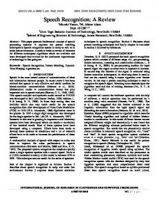
Histogram showing relationship between MLP outputs and percentage correct for each bin. This was generated by collecting statistics from a net with 9 frames of 26 continuous input parameters for a total of 234 inputs, and a 500-unit hidden layer, over the patterns from 1750 Resource Management speakerindependent training sentences and 500 cross-validation sentences. . . . . . . . . . . . . . . . . . . . . . . . . . . . . . 115

7.1

Generic phonemic HMM with a single conditional density estimated on the -th MLP output unit associated with HMM state , and a single state repeated times, where is the average duration of the phoneme. . . . . . . . . . . . . . . . 143 Generic MLP for probability estimation. Hidden layer is used for continuous (real-valued) input , no hidden layer required for discrete (binary) . In the simplest case, is the feature vector from a single frame, but it can include features from surrounding frames as well. The ’s are the classes (associated with HMM states) for which the MLP is trained as a classifier. 144

7.2

9.1 9.2

MLP estimator for left phonetic context, given input, current state, and right phonetic context. . . . . . . . . . . . . . . . . 170 MLP estimator for right phonetic context, given input, and current state. . . . . . . . . . . . . . . . . . . . . . . . . . . . . 171

11.1 RAP node. . . . . . . . . . . . . . . . . . . . . . . . . . . . . 188 12.1 Sensitivity of MLP training to net size. . . . . . . . . . . . . . 197 14.1 MLP with one hidden layer for auto-association. . . . . . . . 211 14.2 Sequence of operations in the auto-associative MLP. . . . . . 212

List of Tables 5.1

Comparison of the recognition error rates (I=insertions, S=substitutions, D=deletions) obtained with 1-state phonemic HMMs with discrete emission probabilities, Gaussian emission probabilities, and outputs of a contextual MLP. . . . . . . . . . . . . . . . . . . . . . . . . . . . . . . .

94

6.1

Phonetic classification rates at the frame level obtained by standard approaches. “Full Gaussian” refers to the case of one Gaussian with full covariance matrix per phoneme, “MLE” refers to the case of one discrete likelihood density per phoneme estimated by counting, and “MAP” refers to the case of one discrete posterior probability density estimated by counting. . . . . . . . . . . . . . . . . . . . . . . 111

6.2

Phonetic classification rates at the frame level obtained from different MLPs, compared with MLE. “MLPa b-cd” stands for an MLP with blocs (width of context) of (binary) input units, hidden units and output units. The size of the output layer was kept fixed at 50 units, corresponding to the 50 phonemes to be recognized. . . 113

6.3

Phonetic classification rates at the frame level obtained from contextual MLPs, compared with standard likelihoods (MLE) and a posteriori probabilities (MAP). R represents the parametrization ratio, i.e., the number of parameters divided by the number of training patterns. . . . . . . . . . 116

6.4

Phonetic classification rates at the frame level on SPICOS obtained from MLPs with linear and nonlinear outputs. . . . . . . . . . . . . . . . . . . . . . . . . . . . . . . . 117

7.1

Word recognition rate on SPICOS database (speaker m003) for different hybrid HMM/MLP approaches (MLP = no division of output values by priors, MLP/priors = division by priors) compared with standard HMMs trained with MLE criterion. . . . . . . . . . . . . . . . . . . . . . . . . . . . . 145 xiii

LIST OF TABLES

xiv 7.2

7.3 7.4

8.1

8.2 8.3

8.4

Word recognition rate on SPICOS (speaker m003) using iterated Viterbi segmentation: MLP/priors = hybrid HMM/MLP approach with MLP output values divided by priors, MLE = HMMs using standard maximum likelihood estimate. . . . . . . . . . . . . . . . . . . . . . . . . . . . . 146 Word recognition rates for 3 speakers on SPICOS, simple initialization of the Viterbi training. . . . . . . . . . . . 147 Context-independent word recognition rate on the speakerdependent DARPA Resource Management (RM) database, no grammar, discrete features. . . . . . . . . . . . . . . . 149 Phonetic classification rate at the frame level and word recognition accuracies of the HMM/MLP approach on speaker dtd05 of the speaker-dependent RM database. FR and WR respectively stand for frame and word classification rate while the next digit (1 or 9) stands for the number of frames used at the input of the MLP. . . . . . . . . . . . . 157 Context-independent word error rates, RM, continuous PLP features. . . . . . . . . . . . . . . . . . . . . . . . . . 158 Recognition accuracies of the HMM/MLP-based classification for the speaker-independent TIMIT database. F and W respectively stand for frame and word classification while the next digit (1 or 9) stands for the number of frames used at the input of the MLP. Accuracies of the Gaussian classifier, when available, are given in brackets. 159 Results using 69 context-independent phone models. The baseline MLP system Y0 uses 69 single distribution models with a single pronunciation for each word in the vocabulary. The DECIPHER system also uses 69 phone models, each with two or three states 200 independent distributions in total. The MLP-DECIPHER system uses DECIPHER’s multiple pronunciation and cross-word modeling. . . . . . . . . . . . . . . . . . . . . . . . . . . . . . . 164

10.1 Comparison of resource requirements for local distance computation in the discrete case: hybrid HMM/MLP and pure HMM.Typical order-of-magnitude values are given for systems with !"# triphone or generalized triphone densities . . . . . . . . . . . . . . . . . . . . . . . . . . . . . . 181 10.2 Comparison of resource requirements for local distance computation in the continuous case: hybrid HMM/MLP (M) and pure HMM (H). . . . . . . . . . . . . . . . . . . . . 183 12.1 Test (and training) scores: 1 cluster, SNR = 1.0. . . . . . 196

LIST OF TABLES

xv

12.2 Test (and training) scores: 1 cluster, SNR = 2.0. . . . . . 196 12.3 Test (and training) scores: 4 clusters, SNR = 1.0. . . . . . 197 12.4 Test Run: Correct (phonemic) frame classification rate for training and test sets. . . . . . . . . . . . . . . . . . . . 199

xvi

LIST OF TABLES

Notation

- $&%' $)(*+,*---*+ /. 1 0 : (acoustic) vector at time 2 -

: dimension of acoustic vectors

- %'3!*+ )( *+ /, *---4*+ . 0 : augmented acoustic vector at time 2 - 0 : transpose operation - 5 : a category or class - 6 : number of classes, HMM states, probability density functions or MLP output classes 0 % 8 7 ;: *---4*+7 .=< : parameters of a discriminant function associated - 7 9 with class 5

- 7 > : : bias of class 5 - ?@%A8 7B( *---*+7 *---*+7DC < : weight matrix - E%A8 F( *---4*+*---4*+HG < : acoustic vector sequence of length I JK

- MLK %A8 $)LK>*---*+H*--- *+=JK < : a subsequence of

of length ONP!

- QR%A8 S ( *--- *+SUT < : set of prototype vectors - V : total number of prototype vectors - W'%A8 S X *--- *+S Z Y * ---*+S \ [ < : prototype vector sequence associated with ; each S [^] Q - _ - d

%A8 à( *--- *+`cb < : the set of possible elementary speech unit HMMs

, d : Hidden Markov models built up by concatenating è ’s

- f , f : parameter set of hidden Markov models d will also be used as Lagrange multipliers xvii

and d ; sometime these

NOTATION

xviii - g : parameter set of all the HMMs in _

- hi%j8 ( *---4* *---* C < : the set of HMM states described in terms of different probability density functions - : a HMM state or an MLP output class (associated with HMM state ) - k : total number of state (with possible repetitions of the same ’s) in a Markov model d - l : mean vector associated with 5 or in the case of Gaussian distribution - m *on : full covariance matrix or covariance “vector” (if diagonal covariance matrix) associated with 5 or - : HMM state observed at time 2

-

: HMM state observed at time 2

L - : HMM observed at the previous time frame

- pA%A8

(

*--- *

*---*

G

< : a HMM state sequence (of length I

)

- rq : local probability or likelihood (or density function) - ts rq : estimate of the local probability or likelihood (or density function) - : local posterior probability - u U : local likelihood - U : prior probability of class (or HMM state) - vwrq : global probability or likelihood (relative to a sequence or subsequence of states or acoustic vectors) - vw ^ d

: likelihood of

given the Markov model d

- vw ^ d : Viterbi approximation of the likelihood of model d

given the Markov

- vwdx : posterior probability of a Markov model d vector sequence

given the acoustic

- vwdx : Viterbi approximation of the posterior probability of d - 2 : number of times a prototype vector S of Q HMM state

given

has been observed on a

- 2 : total number of time state has been observed - 2 : total number of times prototype S has been observed

NOTATION - yzH|{ : “forward” probability %Pvw } +* ( d

xix

G - ~|{ : “backward” probability %Pvw =t J ( } * d

- : number of layers in a MLP - ? } : weight matrix between layer {! and layer { of an MLP - ?

} : augmented weight matrix between layer {P! and layer { of an MLP (taking the bias of layer {^! into account)

- 2 } : number of units on layer { 0 - H $ % 8M( *---4*3 *---*3UC& < : output vector of an MLP as a function of the input pattern

- $ : activation values of the -th output unit of an MLP associated with a class 5 or a HMM state - } : activation vector of the { -th hidden layer of an MLP, given at the input; {D%!*---4*+ - } $ : augmented activation vector of the { -th hidden layer of an MLP (to take the bias into account) - wrq : sigmoid function (applied componentwise if the argument is a vector) - : error function minimized for MLP training; usually, this is a mean square error function or a (relative) entropy criterion -

$ : desired MLP output vector for pattern $ at the input

- : index vector used as desired output vector for MLP training in classification mode; this is a 6 -vector with all components equal to zero except the -th one, which is equal to 1. - $ : index vector of the class assigned to $ - =N! : width of the contextual acoustic information at the input of an MLP ( frames of left context, frames of right context, and the current frame) - : radial basis function L( ) = - M) L * : linear or nonlinear autoregressive function associated with class and applied, at time 2 , on the previous acoustic vectors

- : parameters of the linear or nonlinear predictor associated with class - : order of prediction in AR models - ) : prediction error at time 2 for state (or class)

xx - : number of phonemic contexts * &%!*---*> : the possible phonemic contexts - } - *; *&%!*---4*> : left and rigth phonemic contexts =

NOTATION

Foreword Over the past five years, Hervé Bourlard and Nelson Morgan have been engaged in an international collaboration aimed at determining whether neural networks could be used to improve talker-independent continuous speech recognition. This book provides a detailed review of their successful collaboration. It describes how large multi-layer perceptron networks containing more than 150,000 weights were trained and integrated into a state-of-theart Hidden Markov Model (HMM) recognizer to provide improved acousticphonetic modeling and improved recognition accuracy. The lessons learned along the way form a case study which demonstrates how hybrid systems can be developed that combine neural networks with more traditional statistical approaches. The book illustrates both the advantages and limitations of neural networks as seen by researchers who understand both neural networks and alternative statistical approaches. The book first describes early research and theory which demonstrate that neural networks estimate Bayesian a posteriori probabilities. This allows multilayer perceptrons to be integrated into hybrid HMM speech recognizers via a common statistical framework. The book then describes problems that were encountered and solved in developing hybrid speaker-dependent and speakerindependent continuous speech recognizers. It describes the Ring Array Processor that was required to obtain practical training times on databases with more than a million input feature vectors. It also describes how cross-validation testing was used to prevent over training; how network outputs were normalized by class prior probabilities to provide scaled likelihoods; and techniques that improved training times, including random sampling, correctly initializing output node biases, gradually decreasing the step-size, and trial-by-trial weight adaptation. The book presents some unique network designs and proofs motivated by the connection between networks and statistics. A context-dependent neural network is described which estimates context-dependent class probabilities with many fewer weights than would be required if one output was provided for each class-context combination. This approach requires three small networks instead of one much larger network. A modification of radial basis function networks is also described which forces outputs to sum to one. Proofs are prexxi

xxii

FOREWORD

sented which demonstrate that network outputs estimate Bayesian a posteriori probabilities and that auto-association networks used for data compression perform a function similar to that performed by principal components analysis. This book is useful to anyone who intends to use neural networks for speech recognition or within the framework provided by an existing successful statistical approach. It requires some knowledge of speech recognition and signal processing but provides a helpful case study which demonstrates that neural networks are a useful tool that can be used side-by-side with other more accepted statistical approaches.

Richard Lippmann MIT Lincoln Labs, April 13, 1993

Preface Since Leibniz there has been no man who has had a full command of all the intellectual activity of his day. There are fields of scientific work which have been explored from the different sides of pure mathematics, statistics, electrical engineering and neurophysiology; in which every single notion receives a separate name from each group, and in which important work has been triplicated or quadruplated, while still other important work is delayed by the unavailability in one field of results that may have already become classical in the next field. – Norbert Wiener – At one time, scientific knowledge was held by a relatively small group with a command of an encyclopedic range of topics. Today, it may no longer be possible to do scientific research as a lone wolf. Advances can only be achieved through discussion and worldwide exchanges with scientific colleagues. This is actually a positive development for a number of reasons. First, many ideas can come through the group activity of complementary minds. Past a certain point, participants in such a “group think” exercise are no longer clearly aware of the boundaries of origin of any particular idea. The work reported here is an example of such a collaboration. Secondly, when these advances are obtained through the interaction of colleagues across national lines, this communication is an important component of global awareness. We grow to understand and appreciate each other’s cultures, becoming better citizens of our global village. Finally, widespread exchanges force us toward more effective self-criticism, since we know that others viewing our work will certainly see its flaws. There is, however, a negative side to this distribution of expertise. Innumerable sub-disciplines have developed, often each with its own jargon. This often means that complementary experts may not even share the same technical language, making collaboration difficult. Speech communication with machine is certainly such an area, requiring contributions from linguists, computer scientists, electrical engineers, psychologists, and mathematicians (to name just a few major fields). Even within the engineering aspects of this pursuit, there is xxiii

xxiv

PREFACE

a diverse mixture of signal processing, pattern recognition, probability theory, speech science, and system design. For complete systems, these aspects must be augmented by incorporating knowledge of language. The diversity of these topics is one of the greatest problems for machine speech communication. The work described in this volume is the result of a strong collaboration and friendship between the authors. The joint work began with an extended visit Bourlard made to ICSI starting in 1988, shortly after some seminal work that he had done with Christian Wellekens at Philips in Belgium. After this visit, the research continued both individually and jointly, assisted by frequent short visits, electronic mail, fax, and the occasional expensive phone call. The result was a body of work that we report here, all based on the use of multilayer perceptrons to estimate the probabilities of sound units for use in continuous speech recognition. While only a small part of the overall problem of speech recognition, it nonetheless brings together a range of subjects. We have tried to describe these pieces using consistent terminology, but hope that we still give the reader a sense of the diversity of the fields required to explore this subject. Science moves quickly, and the ideas in these pages may well seem naive in a few short years after they were written. This can’t be helped. On the other hand, some of these ideas may prove to be important, in which case they will almost certainly be misused (that is, be used to Humankind’s detriment). This also cannot be helped. However, we express the hope that the sense of internationalism that was responsible for the research progress will be reflected in the use of this technology for peaceful purposes. Hervé Bourlard and Nelson Morgan Berkeley, CA, May 1993.

Acknowledgments Many people have contributed directly and indirectly to both the work reported here and to this book itself. Some helpful parties will, alas, be unavoidably omitted from any such list.1 Some of the people who we feel most strongly about thanking are (in no particular order):

Richard Lippmann for his Foreword and helpful comments.

Luis Almeida, René Boite, Henri Leich, and John Lazzaro for their early readings and criticism.

Chuck Wooters for the years of work that he has put into developing the practical instantiations of the systems described here

Steve Renals for his work with us, both on writing, theory, and practice.

Christian Wellekens, who collaborated on the work described in parts of Chapters 3 and 7, while he and Bourlard were at Philips.

Marco Saerens, who collaborated on Chapter 13.

Yves Kamp, who collaborated with Bourlard on the work reported in Chapter 14.

James Beck, Phil Kohn, and Jeff Bilmes, who made the RAP machine a reality for the heavy computation required to develop the methods described here.

Yochai Konig, whose criticism was very helpful during our rewrites, and who has been a contributor in the more recent stages of our work.

1

Our friends at SRI: Mike Cohen, Horacio Franco, and Victor Abrash, with whom we have collaborated over the last three years, particularly on the context-dependent advances that they have made; and Hy Murveit, with whom we had early discussions (in 1988) that started off our own collaboration.

We have also gracefully neglected to mention the names of anyone who hindered us.

xxv

ACKNOWLEDGMENTS

xxvi

ICSI in general and Jerry Feldman in particular for putting up with us while we puzzled through this work and this book.

Ditto for Jo Lernout and LHS.

Beatrice Benjamin, for the cartoons that brighten up this sober treatise.

Vivian Balis, for her help with the other figures.

Molly Walker, for her careful editing of the final version.

Of course, we also gratefully acknowledge the recent support from the European Community’s ESPRIT program (Basic Research Project no. 6487), as well as ARPA (and in particular, Barbara Yoon) for support of our collaboration with SRI under ARPA contract MDA904-90-C-5253. We also thank the world’s leaders for not blowing up the planet while we were writing this, as we REALLY wanted to finish it. We thank our families for their support. Finally, we would regretfully like to say farewell to a friend and colleague that left us this year: Frank Fallside, who will be missed.

xxvii

Part I

BACKGROUND

1

Chapter 1

INTRODUCTION New opinions are always suspected, and usually opposed, without any other reason, but because they are not already common. – John Locke –

For thirty years, Artificial Neural Networks (ANNs) have been used for difficult problems in pattern recognition [Viglione, 1970]. Some of these problems, such as the pattern analysis of brain waves, have been characterized by a low signal-to-noise ratio; in some cases it was not even known what was signal and what was noise. More recently, ANNs have been applied to Automatic Speech Recognition (ASR). Despite the relatively deep knowledge that we have about the speech signal, ASR is still difficult. This is so for a number of reasons, but partly because the field is motivated by the promise of human-level performance under realistic conditions, and this is currently an unsolved problem. For speech communication, statistically significant classification accuracies are of no interest if they are low compared to human listeners. So ASR is a hard problem and ANNs can be helpful for hard pattern recognition problems. However, we are wary of assuming that neural “magic” can solve this or any other problem. Practical pattern recognition systems are not realized simply by one monolithic element, either in the form of a single ANN or any other homogeneous component. Solving a real-world problem almost always requires the crafting of a heterogeneous system from modules that the engineer has in his toolkit. This is at least partly because the structure of hard problems themselves is typically heterogeneous. One might have a component that is best described as signal processing, another as a classification or pattern matching module, and yet another might incorporate syntactic or semantic knowledge. ASR is no exception; even for the “standard” statistical systems that we have used as our starting point, complete recognizers consist of a number of critical pieces. This modular property is fortuitous for 3

CHAPTER 1. INTRODUCTION

4

researchers. We can pick some aspect of the whole problem that we consider suboptimal, and attempt to improve it with a new technique (or an old one that has not been applied to this subtask). Ultimately, there are strong advantages to greater homogeneity – for instance, doing the entire task with ANN modules; in principle, this would provide greater flexibility for global optimization of the system. At the moment, we don’t know how to do this. The focus of this book, as suggested by the title,1 is on the integration of ANNs into an ASR system for continuous speech. This has been done for an important recognition subtask, phonetic probability estimation. These probabilities are used as parameters for Hidden Markov Models (HMMs), currently the framework of choice for state-of-the-art recognizers. Keeping the overall framework of a conventional recognizer has permitted us to make controlled comparisons to evaluate new techniques.

1.1

Automatic Speech Recognition (ASR)

The dominant technological approaches for speech recognition systems are based on pattern matching of statistical representations of the acoustic speech signal, such as HMM whole word and subword (e.g., phoneme) models. However, although significant progress has been made in the field of ASR these last years, the typical vocabulary size is still very limited2 and the performance of the resulting systems is still not comparable to that achieved by human beings. Considering the immense effort that has gone into studying speech recognition over the last four decades, one might wonder why this area is still a topic for research. As early as the 1950s, researchers built simple recognizers with credible performance for restricted tasks (such as isolated digits spoken by a single talker). Unfortunately, the techniques used in these systems were not sufficient to solve the general problem of ASR. The difficulties of this problem can be described in terms of a number of characterizations of the task, including: 1. Intra- and inter-speaker variabilities: Is the system speaker dependent (i.e., optimized for a single talker), or speaker independent (can recognize anyone’s voice)? Typically, speaker-dependent systems can achieve better recognition performance than speaker-independent systems because the variability of the speech signal (i.e., the way words and subwords are pronounced) is more limited. However, this is achieved at the cost of a new enrollment (training) session that has to be done for every new speaker; the memory requirements will also be larger since one has to store specific models for every user. 1

See the front cover if you’ve forgotten it. While some existing systems work with very large vocabularies, there is always some compensating restriction, such as the limitation to a very task-specific grammar, for any system that works well enough to be useful. 2

1.1. AUTOMATIC SPEECH RECOGNITION (ASR)

5

For most applications (e.g., the public telephone network), only speakerindependent systems are useful. In this case, speaker independence is usually achieved by using the same baseline models (e.g., HMMs) that are trained on databases containing a large population of representative talkers. In this case, the ASR system does not require specific training and uses the same set of models of every user. A solution between speaker-dependent and speaker-independent systems consists in doing fast speaker adaptation. In this case, starting from pretrained (e.g., speaker-independent) models, one tries to adapt the parameters of the models quickly to better match the characteristics of the user’s voice. This can be performed in a supervised way (e.g., prompting the speaker for a small set of utterances, or taking a corrective action each time the user detects an error) or unsupervised way (from a few unconstrained utterances from the speaker). 2. Is the system able to recognize isolated or continuous speech? With isolated word recognition systems, the talker is required to say words with short pauses in between. This is the simplest case, since word boundaries are detected fairly easily, and since the words are not strongly coarticulated.

Continuous Speech Recognition (CSR) systems can recognize a sequence of words that are spoken without requiring pauses between the words. In this case, the words in the utterances can be strongly coarticulated, which makes recognition considerably more difficult. Typically these systems assume speech with a predefined lexicon and syntax. A very challenging extension of such systems achieves recognition of natural or spontaneous speech, for which the talker is not constrained by vocabulary size or artificial grammatical constraints. This is still an open research issue since, in this case, the system has to deal with speech disfluencies, hesitations, non-grammatical sentences, out-of-vocabulary words, etc. Another problem that is neither isolated word recognition nor continuous speech recognition (but which is as difficult as CSR) is often referred to as keyword spotting (KWS). In this case, one wants to detect “keywords” from unconstrained speech, while ignoring all other words or non-speech sounds. This is a kind of generalization of an isolated word recognition system in which the user is not constrained to pronounce the words in isolation; this leads to more user-friendly systems.3 The challenging problem of rejecting utterances with no keywords is also usually addressed in a KWS system. 3

Diabolical system designers can also use this approach to create a user-nasty system, such as one that reboots whenever the user says “pizza”.


6

3. Vocabulary size and confusability: Is the system able to recognize a vocabulary of only a few words, or can it handle large vocabularies of thousands of words? What is the potential confusability between words? In general, it is difficult to get good recognition results with a large vocabulary, and the computation time can also be an issue in this case. Adding more words increases the probability of confusion between words. Also, since more recognition time is required for a larger lexicon, faster search techniques (e.g., beam search and fast look-ahead) are required, and can degrade the final performance of the system. For large vocabularies, it is also not generally feasible to work with whole word models, since this would require a prohibitive amount of training data, particularly for a speaker-independent system. A natural subword unit is the phoneme, but such units are strongly coarticulated; that is, the pronunciation of each linguistically based sound unit is strongly dependent on its acoustic-phonetic context. In general, ASR performance is significantly affected by the acoustic confusability of the vocabulary to be recognized, which can lead to difficulties even for small vocabularies. This is the case, for example, with the “E” set of the alphabet, that is, for the spoken names of the letters that rhyme with “E” (b, c, d, e, g, p, t, v, and z). 4. Are there any task and/or language constraints? In most cases, the task of continuous speech recognition is simplified by restricting the possible utterances. This is usually done by using syntactic (and, sometimes, semantic) information to reduce the complexity of the task and the ambiguity between words. However, this is still a very active research area since it is not known how to properly interface general grammars and natural speech constraints with acoustic recognizers. The use of semantic information is still an open issue. Since the degree to which these non-acoustic knowledge sources limit the possible utterances can differ, vocabulary size is not a good measure of a CSR task’s difficulty. The constraining power of a language model is usually measured by its perplexity, roughly the geometric mean of the number of words that can occur at any decision point.4 If I is the number of lexicon words, the perplexity v ] !*I . A high perplexity generally implies a high level of difficulty for a task, since many competing word candidates must be examined by the acoustic recognizer. The CSR tasks that will be described in this book will usually have roughly a 1,000 word lexicon and a perplexity equal to 60. 5. Does the system work in adverse conditions? Several variables that can alter the performance of ASR systems have been identified: 4

See [Jelinek, 1990] for a more precise description.

1.1. AUTOMATIC SPEECH RECOGNITION (ASR)

7

environmental noise, i.e., stationary or nonstationary additive noise (e.g., in car, cockpit or on factory floor);

distorted acoustics and speech correlated noise (e.g., reverberant room acoustics, nonlinear distortions);

different microphones (e.g., telephone set, superdirectional or closetalking microphones,) and different filter characteristics (for which the telephone channel is a particular case), which usually lead to convolutional noise;

limited frequency bandwidth (e.g., telephone channels where the transmitted frequencies are limited between approximately 350 Hz and 3,200 Hz);

altered speaking manner, (e.g., Lombard effect, differing speaking rate, speaker stress, breath and lip noise, pitch, uncooperative talker, etc.); or some combination of the above (which is, unfortunately, the most frequent case).

Some systems can be more robust than others in response to some of these factors, but in general recognizers are overly sensitive in this regard.5 6. Will the system be trained to recognize read or natural, spontaneous speech? Virtually all practical applications require the recognition of natural, spontaneous speech. On the other hand, nearly all research experiments have used read text as input (see the ATIS task [DARPA, 1991], an experimental airline reservation system, for a notable exception). The practical difference is a host of disfluencies that people produce – for instance, filled pauses (“um” or “er”) or false starts. Additionally, in natural speech, talkers will almost certainly use some words that are outside of the recognizer lexicon. All of these factors make CSR much more difficult. In this book, we will address the problem of speaker-dependent and speakerindependent CSR for “read” speech, with moderate size lexicons (typically 1,000 words) and a simplified language model with moderate to high perplexities (commonly 60, but much higher for some tasks). This has been chosen as the reference domain for the approach proposed in the book for several reasons:

5

Tests will be performed on standard databases for which results obtained with state of the art systems, highly optimized for these tasks, are available for comparison;

See [Furui, 1993] for a good overview of these variables and the methods that are currently used or investigated to cope with them.


8

These tasks are easy enough to get some “promising” results, but also are hard enough to identify statistically significant improvements or degradations resulting from a new approach; and

1.2

After the developments reported in this book, we were able to integrate our new modules into a state-of-the-art system to boost its general recognition performance.

Limitations in Current ASR Systems

An excellent early report [Davis et al., 1952] described one of the first successful speech recognition systems. While the recognizer worked well, it was limited to recognition of isolated digits for a single speaker. A reading of the text suggests that the authors believed that unrestricted recognition of natural speech was a short hop away. It has been stated for many years that the solution to the speech recognition problem was only five years away.6 Unfortunately, the problem is not that simple. Words that have entirely different meanings (and consequences!) can have very similar phonetic structure. Additionally, words uttered in connected speech are said in very different ways, often including the complete deletion of phonemes that are clearly stated in isolated words (words bounded by silence). There are an infinite number of sentences that may be spoken (since there is no restriction on sentence length), and even an artificial restriction on sentence length (say, to less than 20 seconds) permits a gigantic number of possible word combinations. Each such combination affects the way words and phonemes are spoken (especially due to contextual effects from neighboring sounds). Moreover, as noted earlier, variations in the speech collection environment, such as room acoustics, channel spectral characteristics, or microphone response can all make major changes in the speech spectrum, all of which can seriously degrade recognizer performance. When a system must be speaker-independent, the variability for dialect, speaking speed, and other talker-dependent aspects further increase the difficulty of the task, typically doubling the error rate, even within the same dialect or accent group. Most of these difficulties can be summarized fairly simply: variability of the speech acoustic and variation of additive and convolutional noise. Additionally, however, we instinctively expect a high level of recognition performance, much as would be achieved by a human (or for a keyboard input, for instance), and have very little interest in a recognizer that makes frequent mistakes. For these reasons, speech recognition must achieve a very high level of performance to be of general interest as a man-machine interface. What is the performance currently available from the best speech recognition system? Certainly such systems can give extremely impressive results 6

Since it has been repeated for so long, clearly it must be true ...

1.3. BOOK OVERVIEW

9

in the laboratory, particularly with a task-restricted grammar; 95-98% accuracies have been reported for the recognition of 1000 words in continuous speech [Weintraub et al., 1989; Lee et al., 1989]. However, unconstrained background noise, microphone characteristics, and grammars that are more characteristic of real applications result in far lower performance. Even the relatively simple case of telephone digits, for which rates greater than 99% have been achieved, becomes extremely difficult with the channel variation from real telephone lines; a recent experiment contrasted a 97% accuracy for speaker-independent isolated digit recognition with a 40% score when changes in the telephone channel were not handled [Hermansky, 1990b; Hermansky et al., 1991]. Furthermore, without restrictive grammars (which are not realistic for general speech), even the best speaker-independent systems currently give about 20% word error and about 80% sentence error. This is far from what one would require in a dictation system, for instance. In short, despite encouraging progress over the last few years, speech recognition by machine still has a long way to go to be good enough to be generally useful.

1.3

Book Overview

In this work we will show how neural network techniques can complement traditional approaches to improve state-of-the-art continuous speech recognition systems. However, we will also show that this is not easy; we should not rely too much on the “magical” problem-solving abilities of ANNs without a clear understanding of the underlying principles and tasks. After a basic review of statistical pattern classification (Chapter 2), Chapter 3 recalls the main features and underlying hypotheses of Hidden Markov Models (HMMs), stochastic models that are now widely used for automatic isolated word and connected speech recognition. One of their main advantages lies in their ability to represent the time sequential order of speech signals and the variability of speech production by the use of powerful matching techniques such as the Baum Welch or Viterbi algorithms. The parameters of these models are learned from large data bases that are assumed to be statistically representative. For their training, a critical problem is the choice of a learning criterion. A model is said to be discriminant if it maximizes the probability of producing an associated set of features while minimizing the probability that they have been produced by rival models. Problems related to the choice of a criterion are discussed in Section 3.5. Chapter 4 focuses on linear discriminant functions and a kind of ANN called a Multilayer Perceptron (MLP). Like HMMs, these are learning machines, but they also provide discriminant-based learning; that is, models are trained to suppress incorrect classification as well as to model each class separately. MLPs can acquire pattern knowledge by learning, and can then recog-

10


nize patterns that are similar to those presented in the learning set. This stands in contrast with the HMM approach, which uses a separate model for each phonemic class and usually makes assumptions about the distribution of the associated feature vectors. Further, in contrast to HMMs, MLPs can capture high-order constraints between data while discriminating between classes. However, the sequential nature of the speech signal, which is inherent to the HMM formalism, remains difficult to handle with neural networks. Chapter 5 reviews the different approaches that have been proposed so far to handle sequential signals: models with buffered inputs or recurrent neural networks. Some of these models have already proved useful in recognizing isolated speech units. By their dynamical properties, these models are able to include some kind of time warping, or at least some integration over time. However, ANNs by themselves have not been shown to be effective for large scale continuous speech recognition. It currently appears that a good solution is to integrate them into a statistical framework using standard approaches such as HMMs. To properly interface ANNs with HMMs, it was necessary to understand what these networks are actually computing. In Chapter 6, it is shown that the output values of MLPs may be considered to be estimates of Bayes (a posteriori, or posterior) probabilities when trained for pattern classification. In other words, the MLPs can estimate the conditional probability of each class of speech sound, given the speech data. This property is proved theoretically and demonstrated experimentally on a realistic task. This was an important link between MLPs and HMMs. However, showing that an MLP can generate a posteriori probabilities is not sufficient for recognition, since HMMs require the estimation of likelihoods. That is, standard HMM recognizers require the estimation of the probability of producing the observed data assuming each sound class. Accordingly, a new kind of HMM, referred to as a discriminant HMM, using posterior probabilities instead of likelihoods, is introduced in Chapter 7. While improving the HMM discriminant capabilities, these models preserve the algorithmic aspects of HMMs (e.g., Viterbi-like training and recognition procedures) and have the potential to overcome some of the major weaknesses of standard HMMs. However, it appears that it is not easy to properly interface MLPs and HMMs. Consequently, the modifications of the basic scheme that were necessary to get good word recognition performance are presented and discussed in Chapter 7. In Chapter 7, only discrete features are used. In Chapter 8, the hybrid HMM/MLP approach is extended and tested with continuous acoustic vectors and dynamic features, and this is shown to improve recognition performance. In addition, we show how our approach was successfully integrated into DECIPHER [Cohen et al., 1990], currently (1993) one of the best large vocabulary, speaker-independent, continuous speech recognition systems. This integration improved the performance of a state-of-the-art system. The initial hybrid HMM/MLP approach focused on HMMs that are inde-

1.3. BOOK OVERVIEW

11

pendent of phonetic context, and for these models the MLP approaches have consistently provided significant improvements. In Chapter 9, this approach is extended to context-dependent models. The technique presented is not really constrained to speech recognition; it is a general approach to split any large net used for pattern classification into smaller nets without any assumptions of independence. Since recognizer accuracy is only one measure of a practical speech recognition system, Chapter 10 examines the system tradeoffs for MLP probability estimation and compares the resources requirements (storage, memory bandwidth, and computation) for HMMs, both with and without an MLP. Chapter 11 describes the development of some ANN acceleration hardware and software that were required to speed the research work described in this book. The next part of this book (Part III) discusses related problems or approaches that have been investigated in the framework of this work. In Chapter 12, we describe the approach of cross-validation that has been instrumental in our achievement of good recognition results with a hybrid HMM/MLP hybrid structure. Although this has been done in the framework of speech recognition, cross-validation is a general technique to avoid overfitting when the number of training patterns is not large in comparison with the number of ANN parameters to be learned. In Chapter 13, another kind of hybrid HMM/MLP approach using MLPs as autoregressive models (as initially introduced in, e.g., [Levin, 1990; Tebelskis et al., 1991]) are discussed in the general framework of linear and nonlinear predictive models. In Chapter 14, we investigate the possibility of using MLPs for feature extraction. Auto-associative MLPs have sometimes been proposed for feature extraction or dimensionality reduction of the feature space in information processing applications. This chapter shows that, for auto-association with linear output units, the nonlinearities at the hidden units are unnecessary. This is so because the optimal transformation and the corresponding parameter values can be derived directly by purely linear techniques, relying on singular value decomposition and low rank matrix approximation, similar in spirit to the Karhunen-Loève transform. We conclude the book with Part IV, consisting of a general overview of the final system and the Conclusions. Chapter 15 summarizes the hybrid HMM/MLP approach (including training) that led to our basic system and discusses the possible extensions that are the subject of current research. Chapter 16 contains the conclusions and some speculation about future research trends in the field of ANN-based pattern recognition and speech recognition. In summary, this work describes a first attempt at incorporating neural network approaches for continuous speech recognition. In this attempt we are largely constrained to use neural networks for well defined subtasks. However, the principles established here should be applicable to other parts of speech recognition, and to some extent to quite different tasks in statistical pattern


12 recognition.7

7

But time will tell.

Chapter 2

STATISTICAL PATTERN CLASSIFICATION In this world, nothing can be said to be certain, except death and taxes. – Benjamin Franklin –

2.1

Introduction

No new engineering or scientific technique, however novel, evolves in isolation. Both Hidden Markov Model (HMM) and Multilayer Perceptron (MLP) based approaches have been developed in the context of a long history of pattern recognition technology. Though specific methods are changing, the pattern recognition perspective continues to be useful for the description of many problems and their proposed solutions. While pattern recognition is in general more complex than simply categorizing an input into one of a number of possible classes, the classification perspective is useful. The notation and definitions for this model of pattern recognition will provide tools that permit us to characterize more complex problems, such as speech recognition. In this chapter we will briefly describe the classical elements of pattern classification, with an emphasis on the statistical approach. The definitions and concepts will be useful for understanding the later chapters. Readers with a strong background in pattern recognition may want to scan this chapter quickly.1 Beginners who would like to see a more thorough treatment are referred to [Fukunaga, 1972] and [Duda & Hart, 1973], two truly wonderful books. 1

Or skip it entirely. It’s a short chapter so you won’t miss many jokes.

13

14

2.2

CHAPTER 2. STATISTICAL PATTERN CLASSIFICATION

A Model for Pattern Classification

Many pattern recognition problems can be partially or completely described in terms of the goal of classifying some set of measurements into categories. Many cases are more complex, e.g., deriving a description for a visual scene or translating a speech utterance into a database query. While these problems still are in some sense recognizing a pattern of symbols or values, their solution is far more than the identification of a pattern from some fixed set of classes. Nonetheless, even in such cases there are almost always components of the problem that are well described as either the hard or soft classification of measurements; in the latter case, a graded decision (such as a probability) is required. Generically, a pattern classifier consists of two major pieces: a feature extractor and a classifier. These two modules ultimately have the same goal, namely to transform the input into a representation that is trivially convertible into a class decision. The difference between the two modules is one of perspective. Traditionally the feature extractor is used to convert the raw input into a form that is easily classified; this is a common place to incorporate domainspecific knowledge that will greatly enhance performance over the blind use of automatic techniques. For example, for speech recognition, conversion from a continuous waveform to a series of short-term spectral representations has been shown to be beneficial. This is true despite the fact that, in theory, automatic transformation techniques that are part of the classifier (e.g., neural networks) can learn this mapping. In addition to the representational transformation of the feature extraction stage, this piece of the system typically (though not universally) introduces some coarser granularity. For instance, while the speech waveform might be sampled at 8-16 kHz, the time-varying spectral measure is typically sampled at 100 Hz. This is not necessarily a dimensionality reduction, although transforming to a smaller representation is frequently a motivation for feature extraction; some representations (such as the more complex auditory models for the case of a speech signal) can even increase the signal dimensionality. In either case, the feature extraction stage must produce a representation that is good for separation or discrimination between classes. For the purposes of this book, we will assume a data representation that is discretized in time.2 The features extracted from each chunk of data (e.g., a speech segment) is referred to as a pattern. From these patterns, the feature extractor will produce a sequence of vectors, where each vector component is a variable that has been computed from the original data. We denote this feature vector as %' F( *+H,*--- *+ . , a d-dimensional vector. 3 2 In general, patterns do not need to be part of a sequence, but can be any set of examples that we wish to categorize, such as the set of height and weight values for all American and Belgian speech researchers. 3 In later sections, the feature vectors will also be indexed over time and will be denoted

2.3. STATISTICAL CLASSIFICATION

15

Given a set of feature vectors, the classification stage is designed to discriminate between them on the basis of class. Trained classifiers are developed using a set of feature vector examples, with the object of developing a numerical or symbolic rule that can make the desired distinction for data that has not yet been seen. Typically the training develops a set of discriminant functions, one for each class, which are optimized in an attempt to produce the largest value for the function corresponding correct class. For the purposes of this chapter we will denote 5 *Ow%!*---*6 , as the list of pattern classes. In general, then, we wish to find the best feature extractor and classifier to discriminate between patterns that belong to different classes. For simplicity’s sake, we can define “best” here as the one which provides the fewest classification errors on a new sample of data.4 We have described feature extraction and the classification decision as being distinct processes. We briefly note that it is almost always desirable to integrate these steps as much as possible. For instance, the best features are the ones that are chosen to give good discrimination between classes, and the best classifiers are those that do not critically rely on incorrect assumptions about the feature representation. There are many kinds of pattern classifiers. For the purposes of this book, we will be limited to statistical methods. Statistical pattern classification has the advantage of a powerful mathematical framework.5 Given this framework, we can develop new methods and relate them to existing approaches. It is the capability for such insights that interests us most.

2.3

Statistical Classification

As noted above, statistical approaches provide us with a strong body of relevant theory.6 In the statistical framework, the concept of optimum classification that was discussed in the previous section can be made much more concrete. For some restricted cases, this formulation can even tell us precisely what the optimum classifier must be. More generally, we are given no such prescription; nonetheless, the ideal cases can provide us with some intuition to help understand what new approaches are doing. Using the notation of the previous section, we can denote the probability that a pattern belongs to a class as 5 (where " 5 ! ). Since this expression contains no dependence on feature vectors, and thus can be ¡ Y£¢c¤ ¡ Y +X ¥ ¡ Y>¦ ¥3§r§3§3¥ ¡ Y¨>© . 4

More generally, there is some cost associated with each different kind of error, so that the optimum system in the sense of least cost will not necessarily be the optimum system in the sense of minimizing the number of errors. 5 Unfortunately, the assumptions required for the relevant theory to be valid are almost never realistic. This hasn’t stopped any of us. 6 We assume here that the reader is familiar with the basic ideas of probability, including probability density functions. If not, go directly to jail, do not pass Go, and do not collect $200.


16

expressed before new data is seen, it is generally referred to as the prior or a priori probability of class 5 . If a class probability is conditioned on the feature vector, we can express the probability of class membership given the pattern. In the notation of the previous section, for feature vector this conditional probability is denoted 5 . Since this probability can only be estimated after the data has been seen, it is generally referred to as the posterior or a posteriori probability of class 5 . The generic pattern classification problem can now be stated in a statistical framework: given a set of measurements, vector , what is the probability of it belonging to a class 5 , i.e., 5 ? Intuitively, if one knew these probabilities for all classes and for every possible feature vector, a good decision could be made. As it turns out, such a decision can be formalized and proven to be optimum in the same sense described in the last section. That is, assuming that the pattern must come from one class of 5O( *5t,/*--- *o5C , if we construct a classifier that assigns to class 5 if: 5 «ª

5 *¬®&%!*¯*---/*6°*R ±%

(2.1)

then we can show that such a rule will provide the minimum probability of error for any classifier.7 This would mean that the expected number of errors for a new unseen set of feature vectors would be minimized. In the terminology of the previous section, we would be using 5 (over all values of ) as the discriminant functions. This optimum strategy is often called Bayes’ Decision Rule. Simply put, it requires that we assign a pattern to the class that has the highest posterior probability (i.e., given the vector ). Because of the optimality of this decision rule, the posterior is also sometimes referred to as the Bayes probability. Alas, life is not so simple.8 How do we actually get these probabilities? In general they cannot be computed directly, and can only be estimated from the data (and from assumed prior knowledge). The accuracy of the estimates will ultimately determine the performance of the classifier. Commonly, this estimation is simplified by making some assumptions about the pattern data. For instance, the unknown distributions are often characterized by some parametrized model. In other words, we define the form of the statistical distribution, so that we only have to estimate the parameters, rather than a complete (often continuous) probability density function. Most commonly, we assume this distributional form separately for each class, and for the probability density u 5 = [as opposed to the posterior probability 5 ]. This is the probability density function for the feature vector among those patterns that belong to class 5 , and is often referred to as the data likelihood. This class-conditional data likelihood is simply related to the posterior probability by Bayes’ rule, 7

See Duda & Hart for the proof, which takes about 2 lines of math, but there are some nice text and pictures to make it easy. 8 Or maybe it is, but we just don’t know how to look at it.

2.3. STATISTICAL CLASSIFICATION

17

which is: 5 %

u 5 = 5 %

= = u 5 5 4 / ;C ³ 5 ( 5 ²

(2.2)

where 6 is the total number of classes. In this expression, 5 and are both probability functions or both density functions, according as is discrete or continuous, and 5 and 5 are likewise both probability functions or both density functions, according as 5C is discrete or continuous. In this book, we will mainly make references to probabilities or likelihoods, but we’ll have to keep in mind that these can be actual probabilities or probability density functions. This relation tells us that the posterior probability (or posterior density) is essentially the product of the likelihood function 5 for the observed feature and the prior probability 5 / . The denominator in the formula is just a normalization constant to make the sum over all posterior probabilities equal to 1. The notion of using Bayes’ rule to modify prior beliefs is the essence of “Bayesian” statistics. This somewhat indirect way of calculating the posterior probabilities is not without drawbacks:

Some assumptions are still required about the form of the parametric model of u 5 (see below).

A priori probabilities are generally very difficult to estimate reliably. Using only the likelihood during training (i.e., estimation of the model’s parameters) results in poor discrimination between models.

Using Bayes’ rule, we can reformulate the Bayes’ Decision Rule as follows: assign to class 5 if: u 5 5

5

ª

*¬´&%!*¯*---4*6c*McP ±% 6 5

(2.3)

Note that in this formulation the factor has been factored out. The fraction on the left is commonly referred to as the likelihood ratio. This is also equivalent to using a discriminant function that is the product u 5 = 5 for each value of . In most systems, likelihoods are estimated using the parametric model of a “normal” (or Gaussian) distribution: 5 /

Iµ t*+l *¶m = %

%

!

.¸3, (º¸3,»>¼½ ·

¹m

¾

!

¿l

/ 0

L( = rÁ m À¿l

(2.4)

where l and m respectively denote the mean vector and the covariance matrix associated with class 5 . If the diagonal elements of the covariance matrix , are represented by n , and we assume that the covariance matrix is diagonal


18

(i.e., the measurements of our feature vector are assumed to be uncorrelated), this expression reduces to u 5 /

%jIµ t*+l ¶* m

Â %

.

\³ (

Ã

! , ·n

¾ »>¼½

, Äl Á , n

(2.5)

where l denotes the Å -th component of l . Although it may appear that the choice of this distributional form is arbitrary, normal densities have many useful properties that make them reasonable models. The most obvious is the fact that this distribution is a reasonable approximation to the actual distributions found in many real data sets. This is a consequence of a rule known as the Central Limit Theorem, which says that observable phenomena that are a consequence of many unrelated causes, with no single cause predominating over the others, tend to a Gaussian distribution.9 The Gaussian is also a good approximation of many other distributions. Its most endearing quality is the fact that it is easy to work with – its distribution has been well researched and there is a large pool of knowledge from which to draw when using it. The Gaussian is unimodal; in other words, there is a single “bump” or mode (maximum), which occurs at the mean. More complex distributions with multiple modes can be approximated by weighted sums of Gaussian distributions called Gaussian mixtures. These can be expressed as: 5 = %

Ç

Æ I Èt*+l *¶m 4 ;³ (

(2.6)

where is the total number of Gaussian densities. Parameters are the mixture gain coefficients and are additional parameters to be trained, with the constraints: ´É

"*

and Ç

Æ %!*¬ww%!*---4*6 ;³ (

For each of these expressions, there are a number of parameters that must be estimated from the data. In the case of a single Gaussian, this is trivial if the classes are known; once the means and covariances are estimated for each class, the work is done. In the case of the mixture, the parameters cannot be determined so directly, since the means and are not a priori associated with a particular subset of the feature vectors. However, all of the parameters of (2.4), (2.5) and (2.6) can be iteratively determined by the powerful “Estimate and Maximize” (EM) algorithm [Dempster et al., 1977; Baum, 1972]. This 9

This was proven by Markov, which shows that he did more than assemble chains.

2.4. PATTERN CLASSIFICATION WITH REALISTIC DATA

19

approach is guaranteed to iteratively converge to a local minimum of some measure of error between the model and the sample distribution of the data. By adopting models for the conditional probability 5 / based on standard distributions like (2.4), (2.5) or (2.6) and applying Bayes’ rule, we can define a relatively straightforward statistical classifier. The performance will depend on how closely the pattern data does actually fit the model selected, but generally Bayesian classifiers based on simple parametric assumptions can perform well. In passing, it might be important to recall here that if the likelihoods u 5 are assumed to follow Gaussian distributions, the posterior probabilities 5 generally do not have Gaussian-like distributions at all [Duda & Hart, 1973]. For the case of Gaussian distributions like (2.4), it can be shown that a quadratic decision surface is provided by the Bayes classifier; this can be seen by using log likelihoods and priors in the discriminant function rather than the densities themselves. In this case the exponential of the normal distribution drops away, leaving only first and second order functions of the feature vector. If a further assumption is added, namely that the class distributions have equal covariance matrices, it can also be shown that a linear classifier is optimal; this is demonstrated in Section 4.2.3. Note that this constraint is equivalent to the assumption that the distributions both have the same overall shape, spread and correlation between features. In general, a linear classifier can be useful for other distributions, though it is not optimal. Because if its simplicity, it can be derived in many ways, including through deterministic procedures. In later chapters it will be shown that neural networks can be seen as generalizations of these simpler pattern classifiers. They can form more complex and unconstrained decision surfaces, and so do not require strong assumptions about the pattern distributions. However, in many cases it is useful to view the network’s operation in terms of the simpler techniques described in this chapter, in other words, as approximations to a Bayes’ classifier.

2.4

Pattern Classification with Realistic Data

The distinction between training and testing data is a critical one for pattern classification. In some simple examples of function learning (such as the famous XOR problem) a relationship that can be explicitly stated for the complete set of possible feature vectors is learned. However, in classification problems we often have a huge or even infinite number of potential feature vectors, and the system must be trained using a very limited subset that has been labeled with class identity. Thus, even though the relationship between feature vector and class might be learned perfectly for some training set of data, this will not in general mean that the likelihoods or posteriors are well-estimated for the general population of possible samples. In general, the classification error on the training set patterns should be

20


viewed as a lower bound. A better estimate of the classifier error is obtained using an independent test set. The larger this test set, the better the representation of the general population of possible test patterns. Conventional significance tests (e.g., a normal approximation to the binomial distribution for correctness on the test set) should be done as a sanity check. For instance, a 49% error on a million-pattern test set is significantly different from chance (50% error) on a two-class problem; it represents 10,000 patterns. On the other hand, the same error percentage on a 100-pattern test set is indistinguishable from chance performance.10 One way to effectively increase the size of a test set is to use a “jackknife” procedure, in which each split of the data (e.g., fifths) is used in turn for test after using the remaining part for training. Thus, all of the available data is ultimately used for the test set. Training set size is also a major concern for real problems. The larger the training set, the better the classifier will do on representing the underlying distributions. Also, the more complex the recognizer (e.g. the larger the number of independent parameters), the greater the risk of over-specializing to the training sample, and generalizing poorly to independent test sets. Both of these factors push pattern recognition researchers toward using as much training data as possible. Unfortunately, in most practical situations, there are strong limits on the available data. In this case, clever approaches to squeezing out information from limited data are essential, whether they are based on domain-specific knowledge, or on general constraints that diminish the tendency for the classifier to “over-learn” the training set.11 Another difficulty associated with the finite size of the training set concerns the discriminant character of a statistical classifier. As noted in the previous section, likelihoods and posteriors are simply transformable between one another (by Bayes’ rule). However, in the case of probability estimates (as opposed to true probabilities), the training criterion will produce different results. For instance, if the probabilities are estimated in a procedure that attempts to maximize the discrimination between classes, the classification error will be minimized. This might actually produce poorer estimates of the likelihoods than would be observed after training by a criterion that attempts to best model the underlying densities u 5 = . This would not be the case for an infinite amount of training data, for which the estimates could converge to the true underlying distributions, so that Bayes’ rule would literally be satisfied and the criteria would be equivalent. In general, making strong assumptions about the data (such as the Gaus10

For the normal approximation to a binomial distribution, the equivalent standard deviation is Ê ËÌ , where is the number of patterns, Ë is the probability of getting the class correct by chance, and Ì is the probability of getting the class incorrect by chance. For the examples above, this would be 500 and 5 patterns, respectively. 11 In chapter 12, we describe such a general form of training constraint, called crossvalidation. In this approach, training is modified so that generalization performance is guaranteed never to become worse.

2.5. SUMMARY

21

sian assumption discussed in this chapter) improves the quality of the estimate – IF the assumption is correct. To the extent that these assumptions are wrong, the resulting estimates are poor. Approaches such as EM estimation of mixture Gaussians and gradient-based neural network training incorporate successively weaker constraints, and thus have largely supplanted the earlier, simpler models (e.g., single Gaussians per class). Speech recognition requires the incorporation of “soft” classification decisions as part of the more global decision about the utterance. This requires a dynamic model that represents sequences, rather than the static pattern classification described in this chapter. A general statistical framework for this more general case is presented next.

2.5

Summary

In this chapter, we have very briefly introduced the basic notions (and notations) of feature extraction and statistical pattern classification that will be used in this book. Ideally, the feature extractor and the classifier should be jointly optimized. However, in most cases, these processes are developed independently of each other. Statistical classification should rely on the posterior probability. However, since this probability cannot generally be estimated directly from the data (parametric models are not known, and there is not enough training data to estimate the priors implicitly included in it), it is usually replaced by a likelihood criterion, which will be good only if the assumptions made about the distribution of the data are correct. Also, the use of likelihoods instead of posterior probabilities will result in poorer discrimination properties.

22


Chapter 3

HIDDEN MARKOV MODELS Everything should be made as simple as possible, but not simpler. – Albert Einstein –

3.1

Introduction

The most efficient approach developed so far to deal with the statistical variations of speech (in both the frequency and temporal domains) consists in modeling the lexicon words or the constituent speech units by Hidden Markov Models (HMMs) [Baker 1975a,b; Jelinek 1976; Bahl et al., 1983; Levinson et al., 1983; Rabiner & Juang, 1986]. First described in [Baum & Petrie, 1966; Baum & Eagon, 1967; Baum, 1972], this formalism was proposed as a statistical method of estimating the probabilistic functions of Markov chains.1 Shortly afterwards, they were extended to automatic speech recognition independently at CMU [Baker, 1975b] and IBM [Bakis, 1976; Jelinek, 1976]. Speech is a non-stationary process, but it is assumed to be “quasi-stationary.” That is, it is assumed that over a short period of time the statistics of the speech do not differ from sample to sample. Under this assumption a preprocessor can extract statistically meaningful acoustic parameters (feature vectors) at regular intervals from a sampled speech waveform. Typically the original speech is sampled at 8 to 16 kHz (8 for telephone speech and 16 or so for high-quality microphone input). The features are commonly extracted once per 8-16 msec, and are calculated from a 20 to 30 msec analysis window. Many variants of spectral analysis have been used, including Linear Predictive Coding (LPC), Perceptual Linear Prediction (PLP) [Hermansky, 1990a], and log power spectral or cepstral coefficients computed from a spectrum with “mel scale” spacReminder: a Í -th order Markov chain is a sequence of discrete random variables that depends only on the preceding Í variables. For HMM systems, typically Í is 1. 1

23

24

CHAPTER 3. HIDDEN MARKOV MODELS

ing, which roughly corresponds to auditory critical bands. Physiologicallybased auditory models have also been developed by a number of researchers and are summarized in [Greenberg, 1988]. Simpler models based on some gross psychoacoustic characteristics that display some robustness to the channel characteristic were described in [Hermansky et al., 1991]. First and second time derivatives of spectral or cepstral parameters between successive time slots are also often added to the speech features to represent some of the speech dynamics [Furui, 1986; Lee, 1989]. These derivatives may be calculated by a simple differencing operation or by polynomial approximation to the derivative (since differencing is inherently very noisy). These “delta features” provide information about spectral changes over time, although their exact interpretation is still not entirely clear. Whatever the acoustic features are, the feature extraction process converts the speech signal into a sequence of acoustic vectors 9%8 ( *+ , *F--- *Î G < . For a good review of the basics of digital processing of speech signals, see [Rabiner & Schafer, 1978]. Hidden Markov modeling assumes that the sequence of feature vectors is a piecewise stationary process. That is, an utterance is modeled as a succession of discrete stationary states, with instantaneous transitions between these states. Essentially, a HMM is a stochastic finite state machine with a stochastic output process attached to each state2 to describe the probability of occurrence of some feature vectors. A simple HMM is illustrated in Figure 3.1. Thus we have two concurrent stochastic processes: the sequence of HMM states modeling the temporal structure of speech; and a set of state output processes modeling the (locally) stationary character of the speech signal. The HMM is called “hidden” because the sequence of states is not directly observable, but affects the observed sequence of events. Ideally, there should be one HMM for every sentence allowed in the recognition task. However, this is clearly infeasible, so that a hierarchical scheme must be adopted. First, a sentence is modeled as a sequence of words. The total number of models required is then much smaller. However, to further reduce the number of parameters (and, consequently, the required amount of training material) and to avoid the need of a new training each time a new word has to be added to the lexicon, sub-word units are usually preferred to word models. Although there are good linguistic arguments for choosing units such as syllables or demi-syllables, the unit most commonly used is the phoneme. This is the unit used in this work, in which we will use between 60 and 70 phoneme models.3 In this case, word models consist of concatenations of phoneme models (constrained by pronunciations from a lexicon), and sentence models consist of concatenations of word models (constrained by a grammar). 2 More generally, the stochastic process could be regarded as being attached to the transitions – see Section 3.3 for more details about this. 3 In fact, we generally use categories that are more like phones, i.e., acoustic categories, whereas phonemes are linguistic categories.

3.1. INTRODUCTION

25

p(qi | qi)

p(qj | qj)

p(qj | qi)

qi p(xn | qi)

qj p(xn | qj)

xn

xn

Figure 3.1: A schematic of a two state, left-to-right hidden Markov model (HMM). A hidden Markov model is a stochastic automaton, consisting of a set of states and corresponding transitions between states. HMMs are hidden because the state of the model, , is not observed; rather the output, the acoustic vector of a stochastic process attached to that state, is observed. This is described by a probability distribution . The other set of pertinent probabilities are the state transition probabilities ¶ . By the late 1980’s, a number of laboratories were able to demonstrate large-vocabulary (1,000 words), speaker-independent, continuous speech recognition systems based on HMMs [Lee, 1989; Weintraub et al., 1989; Paul, 1989]. These systems extended the earlier HMM approaches in several ways, such as:

better modeling of speech dynamics, by extending the feature vectors to first and second time derivatives;

adding phonological rules; and better speech units such as context-dependent phoneme models (e.g., biphones and triphones).

Although this kind of approach is very efficient and can lead to very impressive results in the laboratory, the numerous implicit assumptions that make optimization of these models possible limit their generality. In this chapter, we will briefly recall the fundamentals of standard HMM approaches by making explicit all the underlying assumptions. The algorithms used to evaluate their parameters and to perform decoding will also be recalled. For reviews and further reading on the fundamentals of HMMs, see [Baker 1975a,b; Jelinek, 1976; Bahl et al., 1983; Levinson et al., 1983; Rabiner & Juang, 1986; Rabiner, 1989; Lee, 1989].


26

This chapter is not intended to present a deep description of HMM-based speech recognition and training algorithms, but only to give the preliminary body of knowledge necessary for this book. Its primary goal is also to list the many implicit assumptions that are made when using HMMs and that led us to use neural networks to try to alleviate some of these. For more details about the subject, we recommend [Deller Proakis & Hansen, 1993], a recent book that gives a very good (and detailed) overview of the most common speech analysis methods, and a very clear description of the theoretical developments related to HMMs.

3.2

Definition and Underlying Hypotheses

In the HMM formalism, the speech signal is assumed to be produced by a finite state automaton built up from a set of 6 states hÏ%A8 ( * , *---* C < governed by statistical laws and (non-emitting) initial and final states T and Ð . Each speech unit (e.g., each vocabulary word or each phoneme) is associated with a Markov model made up of states from h according to a predefined topology. Markov models of words or sentences can then be built up by concatenating (according to phonological rules) elementary speech unit models. %Ñ8 à( *--- *+`cb < represent the set of possible elementary speech Let _ unit HMMs and ÒÓ%Ó8/Ô( *---*¶ÔHb < the set of associated parameters. In the following, d (or d ) will represent the HMM associated with a specific word or sentence (or ) and obtained by concatenating elementary HMMs of associated with the speech units constituting and made up of k states _ } ] h with {°%Õ!*F--- *k . The same state may occur several times and with different indices { , so that kAP ±% 6 . The set of parameters present in d (or d ) will be denoted Ò (or Ò ) and is a subset of Ò The key training and decoding criterion of HMMs is based on the posterior probability vwdx that the acoustic vector sequence has been produced by d . During training, we want to determine the set of parameters Ò that will maximize vwdÑ c*¶Ò for every associated with d ; this is usually referred to as the Maximum A Posteriori (MAP) probability criterion. During recognition, we have to find the best d that maximizes vÀdÑ c*¶Ò given a fixed set of parameters Ò and an observation sequence . Unfortunately, the training process usually does not permit characterization of vwdx directly but only the probability that a given model will generate certain acoustic vector sequences, i.e., vw Ö d .4 Using Bayes’ law, vwdx can be expressed in terms of vw Ö d as vwdx 4

%

vwd v w

vw Ö d

See discussion in Chapter 2 and consequences of this in Section 3.6.

(3.1)

3.2. DEFINITION AND UNDERLYING HYPOTHESES

27

in which vw Ö d is usually referred to as the likelihood of the data given the model d , vwd is the prior probability of the model (usually given by the language model), and vÀ is the prior probability of the acoustic vector sequence.

First set of hypotheses:

H1: It is usually assumed that vwd can be calculated separately (i.e., without acoustic data). In continuous speech recognition, d usually represents a sequence of word models for which the probability vwd can be estimated from a language model, usually formulated in terms of a stochastic grammar. However, if d represents elementary HMMs representing phonemes, the lexicon and the grammar together make up the language model, specifying prior probabilities for sentences, words and phones. This will be discussed further in Section 7.8.

H2: For a known sequence of observations, vw can be assumed constant since it does not depend on the models. However, we will in Section 3.6 that this is only true if the model’s parameters are fixed.

In this case, estimation of (3.1) amounts to calculating vw Ö d , the probability that d has generated the acoustic vector sequence . When used for training this criterion is usually referred to as the Maximum Likelihood Estimate (MLE) criterion, emphasizing that optimization (i.e., maximization of vÀ Ö d ) is performed in the parameter space of the probability density functions or likelihoods.5 As discussed in Section 3.6, a consequence of this assumption is that, during training, vw ^ d will depend only on the set of parameters Ò present in d [which will sometimes be made explicit by writing vw ^ d×*¶Ò ] while vwdÑ was dependent on the whole set of parameters Ò [which will sometimes be made explicit by writing vwdx °*¶Ò ]. Given this formulation, three problems have to be addressed when using HMMs for speech recognition (see [Rabiner & Juang, 1986; Lee, 1989] for an extended development on this theme):

Parametrization and estimation of probabilities – How should vw Ö d be computed, and what are the necessary assumptions about the HMMs to define a useful parameter set Ò ?

5

Training problem – Given a set of observation sequences , '% !*---4*> , associated with their respective Markov models d , how should the model’s parameters be determined so that each model has the highest

ØÙZÚÜÛ Ý°Þ is not a probability, but rather a probability density function (pdf).


28

possible probability vw d *¶Ò 4 of generating its associated observation sequences, i.e., ßàáUâwß Â Ò

¼

¶³

Æ (

vw d

*¶Ò 4

However, it is important to remember here that, ideally, the parameters should be determined so that they maximize vÀd *¶Ò since this is a discriminant criterion that actually minimizes the error rate (recalling Chapter 2; also see discussion in Section 3.6).

3.3 3.3.1

Decoding problem – Given the set of Markov models with their trained parameters and a sequence of observations , how should the best sequence d of elementary Markov models be found to maximize the probability that d generated the observations?

Parametrization and Estimation General Formulation

The estimation problem can be stated as: given a Markov model d , compute the probability vw Ö d that it will generate the sequence of acoustic vectors ã%ä8 F( *$,/*F--- *ÎG < . Starting from the actual likelihood criterion we will show the hypotheses that are necessary to make the model computationally tractable. G : We define a path å of length I in the model as an ordered sequence p ( % ( , G GæJt( 8 % * *---4* * % Ð < of I states (non-emitting initial and T * final states excluded) entering via the initial state T and ending via the final state Ð of d . Both initial and final states are assumed to be non-emitting states (i.e., no acoustic vectors are associated with them).6 Along this path, ] represent the HMM state at time 2 , with let h , and let mean that specific state is visited at time 2 . If å denotes the set of all possible paths ç in d , the actual calculation of vÀ Ö d involves summing the probabilities of all possible paths ç ] å , i.e.: vw ^ d

Ç èºé)ê %

vwÈåO*+Ö d

%

Ç èºé)ê

G vwp ( *+Ö d

(3.2)

G

where p ( is the particular state sequence associated with a specific path å . To make apparent all possible paths, (3.2) can also be rewritten (without any simplifying assumptions) as: vÀ Ö d 6

%

Ç

Ç ( G ---ìë vw } X * --- * } [ *+^ d } X ³ ( } [³ ( ë

As shown later, these states will be used only to initialize recursions.

(3.3)

3.3. PARAMETRIZATION AND ESTIMATION

29

( G for all possible 8 } X *---* } [ < ] å . Since events } are exhaustive and mutually exclusive, i.e.: Ç

ë vw } %!*¬$2 } ³ (

probability vw ^ d can also be written for any arbitrary 2 and without any simplifying assumptions: àß=M ï ð Ç

%

vw Ö d

ë vw } +* Ö d }³ (

*uí î 2

]« !*I

(3.4)

where vw } *+Ö d denotes the probability that is produced by d visiting state } at time 2 and can also be written as:7 vw } +* Ö d

%jvw } +* ( d

vw G Jt( } +* ( *d

while (3.5)

where ñ denotes the partial vector sequence 8 ñ *Î ñ Jt( *z--- *Î . In this expression, vw } *+ ( d represents the joint probability of having generated the partial observation sequence ( and having arrived at state } at time 2 given HMM d ; this probability will be defined as the forward probability yzH in Section 3.3.4 [equation (3.13)]. G

} vw =Jt( *+ ( *d represents the probability of the partial observation seG quence Jt( given that the partial observation sequence ( has already been observed while arriving at state } at time 2 ; this probability will be defined as the backward probability in Section 3.3.4 [equation (3.15)]. It is then easy to show that, without any assumptions, the following recursion holds: vw } +* ( d

%

Ç

)L( )L( ë vw *+ (

d ³ (

} +* ML( *+ )L( *d (

(3.6)

which will be defined later on as the forward recursion of the Forward-Backward algorithm [Baum, 1972; Bourlard et al., 1985; Lee, 1989] (see Section 3.3.4 for further discussion). In many texts, notations vwrq and rq stand for actual probabilities and probability density functions respectively. However, in this book, we will assume that the reader can infer which is referred to, and will instead use vwrq to denote “global” or “accumulated” probabilities or densities (where the lefthand side of the conditional contains a sequence of acoustic vectors or a sequence of HMM states) while rq will stand for local probabilities (i.e., relative to a specific acoustic vector and/or a specific HMM state). ML( ML(

in (3.6) is usually The conditional probability } *+ *+ ( *d referred to as the local contribution. To make the models computationally 7

Throughout much of this book, the following “trick” which ¥ ó Û ô+Þ is used, ó¶¥ is ó essentially a restate¢ Ë ÙZò)Û ô3Þ Ë Ù Û ô3Þ . This decompoment of the definition of conditional probability: Ë ÙZò sition proves very useful in understanding the progression through many of the equations.

30


tractable, the influence of the conditional events are usually limited by some simplifying hypotheses. For example, the dependence is restricted to the last emitted vector; this could be achieved by concatenating two successive vectors as in [Furui, 1986] and in [Marcus, 1981, 1985], while an explicit formulation is given in [Wellekens, 1987]. However, in standard HMMs [Bourlard et al., 1985; Jelinek, 1976], the local contribution is assumed independent )L( of the whole previously emitted vector sequence ( and thus reduces to ML( } *+$

*d . This is equivalent to assuming that, not only are the acoustic vectors uncorrelated, but also the Markov models are first-order Markov models. Indeed, to make these new assumptions more explicit, let us rewrite (first without any of these assumptions) the local contribution in (3.6) as: ML( L( ) } +* $ *+ ( *d )L( ML( %« } +* ( *d

)L( )L( F } * *+ ( *d

(3.7)

Actually, equation (3.7) reflects the property that hidden Markov models can in fact be described in terms of two correlated Markovian processes, one corresponding to the state sequence, and the second one to the acoustic vector sequence. This explains why HMMs are called “hidden” Markov models since there is an underlying Markov process (i.e., the state sequence) which is not observable, but affects the observed Markov process describing the sequence of events. It is then clear that, when assuming that the local contribution in )L( , two hypothe(3.6) is independent of the past acoustic vector sequence ( ses are actually made (one for each underlying Markov process), i.e.:


31

Second set of hypotheses:

H3: It is assumed that Markov models are first-order Markov models, i.e.: ML( ML( ML( } *+ ( *d %E } *d (3.8) which states that the probability that the Markov chain is in state } at time 2 depends only on the state of the Markov chain at time 2µ ! , and is conditionally independent of the past (both the past acoustic vector sequence and the states before the previous one). Probabili ML( ties } *d *¬H*3{%õ!*---4*k , are usually referred to as transition probabilities and represent the probability to go from to } in a Markov model d . Since these transition probabilities are usually assumed to be stationary (models are usually assumed to be time invariant), the upper time indices will be dropped in the following when there is no risk of confusion. Although these transition probabilities are usually dependent on d , this conditional will sometimes be overlooked in the following when considering a specific HMM. These transition probabilities are nonnegative (of course!), and the probabilities of all transitions that leave a state sum to one, i.e., Ç

ë } *d ³} (

%!*Î¬ö%!*---*k

for every specific d . These probabilities can be estimated during training by counting the relative occurrence of state transitions.

H4: Another common related assumption is the observation-independence assumption, i.e.: ML( ML( $ } * *+ ( *d

)L( %E } * *d

(3.9)

which states that the acoustic vectors are not correlated or, in other words, that the probability that a particular acoustic vector will be emitted at time 2 depends only on the transition taken at that time (from )L( state to } ), and is conditionally independent of the past. Probabil)L( ities } * *d are usually referred to as emission-on-transition probabilities [Jelinek, 1976] and represent the probability of observing $ while doing a transition from state to } . Given these two assumptions, the local contribution in (3.6) thus reduces to ML( ML( } +* *+ ( *d

%« } *d

ML( $ } * *d

Given this formulation, one other assumption is commonly made:

(3.10)


32

H5: Although emission-on-transition probabilities are sometimes used as such [Jelinek, 1976; Lee, 1989], they are often assumed to depend ML( only on the current state (independent of the previous state and of the model d ) to reduce the number of parameters, i.e., ML( $ } * *d

%÷ }

(3.11)

in which case the $ } ’s are simply referred to as emission probabilities. Since these emission probabilities are usually assumed independent of the model, d has been removed from the conditional.8 Also, since the models are assumed time invariant, the upper time indices of the states will generally be dropped when they are not required for clarity. L Notation like } and will sometimes be used to remind the reader that state was the state visited before } . Taking hypotheses H3-H5 into account, (3.6) reduces to: vÀ } +* ( d

Ç )L( ML(

%õø *+ (

d ë vw ³ (

} *d

1ù }

(3.12)

which is the basic recursion of HMMs. To compute the emission probabilities of (3.12), each state of h (or each pair of states in the case of emission on transitions) has to be associated with a probability density function describing / . Since the acoustic vectors $ are often in the form of d-dimensional real-valued feature vectors, additional hypotheses about the underlying probability density function describing these emission probabilities are usually required.

3.3.2

Continuous Input Features

Let represent a sequence of acoustic vectors 8 F( *--- *+$$*--- *+G < , where each $ belongs to a predefined d-dimensional feature space (e.g., cepstral vectors). To estimate the emission probabilities, some assumptions about the underlying distribution associated with each state are required. In the case of continuous input, it is particularly useful to split the local contribution as done in (3.10), since this leaves only the continuous random variable on the left-hand side of the conditional in the emission probabilities.

H6: As mentioned in Chapter 2, in many practical situations $ } in (3.12) is estimated by assuming it to be in the form of a multivariate Gaussian distribution (2.4). To reduce the number of free parameters, the

8 This is usually referred to as state tying between models, i.e., a state Ìú is described in terms of the same probability density function independently of the model Ý it belongs to. If we do not assume that the emission probabilities are independent of Ý , this is then equivalent to specific states with probability density functions for every possible Markov model Ý .


33

components of the feature vector are often assumed to be uncorrelated (i.e., the covariance matrix is assumed to be diagonal), so we can compute by (2.5). Since the normal distribution with a diagonal covariance matrix is generally not a good enough model, emission probabilities are often estimated from multivariate Gaussian mixture densities (2.6) [Rabiner et al., 1985]. Other forms include the Gaussian autoregressive mixture density [Juang & Rabiner, 1985], the Richter mixture density [Richter, 1986], and the Laplace mixture density [Ney & Noll, 1988]. Whatever solution is chosen, assumptions are made about the underlying probability density functions. Although it can be proved that a mixture of Gaussians can model any kind of distribution, we still do not know how many Gaussians are needed per state, and the number that we can effectively train will be dependent on the size of the available training set. A problem worth noting in all these approaches is that the probability is usually not computed but is simply replaced by the value of the probability density function on instead of estimating the actual probability, i.e., the integral of the pdf on cµ *+Nû+ . However, if is small enough, the actual probability is then equivalent to the density within a scaling factor equal to = . This problem does not appear in the case of discrete input features.

3.3.3

Discrete Input Features

In discrete HMMs, the acoustic vector sequence is quantized in a front-end processor where each acoustic vector $ is replaced by the closest (in the sense of Euclidian or Mahalanobis distance) prototype vector S selected in a predetermined finite set QR%A8 S( *--- *+S *--- *+S T/< of cardinality V . Usually, Q is referred to as the codebook of prototype vectors. This prototype vector set is usually determined independently by using clustering algorithms, e.g., K-means or binary splitting algorithms, on a large number of acoustic vectors [Linde et al., 1980; Makhoul et al., 1985]. In this case, the acoustic vector sequence is replaced by a (prototype) vector sequence W'%A8 S X *---*+S ZY *---4*+S Z[ < , where Å represents the label of the closest prototype vector of Q associated with . Consequently, emission probabilities can be described in terms of discrete probability density functions, and every L-state Markov model is characterized , by Vwk parameters S

L

} *

for Åü%ã!*---4*V and H*3{%ã!*---4*k , if emission-on-transition probabilities are used [i.e., the left-hand side of (3.11)], or by Vw°k parameters S }


34

if we assume that the emission probabilities depend only on the current state [right-hand side of (3.11)].9

H7: In the discrete case, we do not require hypothesis H6 about the underlying distribution of the emission probabilities. However, there is a similar assumption about the distribution of the feature space that is implicit in the choice of distance metric for the clustering procedure (e.g., the Euclidian distance measure in the case of the K-means clustering algorithm).

Additionally, if multiple features are used, quantization distortion is reduced if separate codebooks are used; however, since the resulting probabilities are combined by multiplication, there is an implicit assumption of feature independence. In the case of continuous HMMs, there is no need to choose the distance metric or vector quantization heuristics. The parameters of the models are computed directly but at the cost of limiting assumptions regarding the form of the probability density function. In a common form of these assumptions, Gaussians or Gaussian mixtures are used with covariance matrices having nonzero elements only on the diagonal. This is equivalent to assuming that the features are uncorrelated. In today’s speech recognition systems, the choice between discrete and continuous HMMs often depends on several factors:

Compared with discrete models, continuous distributional models usually require fewer parameters, which limits their memory requirements.

Since they have fewer parameters, continuous distributional models usually require less training data to achieve good generalization performance. However, if enough training data is available (which is rarely the case!), discrete models can give a better estimate of the observation density function. Generally, continuous HMMs require longer training and recognition time. Continuous models require the calculation of several Gaussian or multi-Gaussian densities. For discrete HMMs, probability calculation is replaced by a look-up table and only quantization of the acoustic vectors has to be performed (which can be optimized by tree-search approaches like binary splitting).

An intermediate approach uses what are referred to as semi-continuous HMMs, and aims at incorporating the advantages of both discrete and continuous HMMs while keeping the number of parameters and the computation time 9

Again, if these discrete emission probabilities are assumed to be independent of the Markov ¦ model Ý (i.e., tied emission probabilities), the total number of parameters in these two cases will be respectively equal to ýoþÿ and ýoþ ÿ .


35

acceptable. Essentially, semi-continuous HMMs use a “codebook” of Gaussians shared by all output pdfs associated with ] h . See Section 6.7.2 for a further discussion and extension to the relationship with ANNs.

3.3.4

Maximum Likelihood Criterion

The problem considered here is the following: given a set of model parameters, how do we compute the likelihood vw ^ d (3.2) of an acoustic vector sequence given a Markov model d ? Unfortunately, direct computation of G (3.2) is clearly infeasible since the number of operations is I k (see [Rabiner, 1989] for the full calculation).10 The so-called Forward-Backward algorithm [Baum & Eagon, 1967; Baum, 1972] can be used to efficiently compute vw Ö d . This is achieved by splitting vÀ Ö d into a sum of products of a “forward” and a “backward” probability [as done in (3.4) and (3.5)]. Considering (3.5), we may define the forward probability yzH|{ %Pvw } +* ( d

*Î¬${ ]

!*k

(3.13)

as the joint probability of having generated the partial observation sequence ( %'8 F( *---*+ < and having arrived at state state } at time 2 given HMM d . In this case, recursion (3.12) [i.e., recursion (3.6) after hypotheses H3-H5] can be rewritten as: yzJt(|{

Ç ø&ë ³ %

(

yzH } 1ù =Jt(4 } Î * ¬{ ]

!*k

(3.14)

and is often referred to as the forward recursion of the Forward-Backward algorithm. By definition of yzH|{ , it is clear that recursion (3.14) is initialized by setting y (|{ %µ F(/ } } T *¬{ ]

!*k

where T is the initial (non emitting) state of d . In a similar way, and considering the second factor in the right-hand side of (3.5), we can define the backward probability ~|{

G %jvw =Jt( } +* ( *d

(3.15) G

as the probability of the partial “backward” observation sequence Jt( % 8 =Jt( *--- *+G < , given that the partial observation sequence ( has already } been observed while arriving at state at time 2 . The corresponding backward recursion of the Forward-Backward algorithm is then: ~|{ There are necessary. 10

[

%

Ç ³

ë (

} $Jt(4 = ~=Jt(4 *¬{ ]

!*ku

possible state sequences, and for each of them about

(3.16) computations are


36

à

with the initialization ~ G |{ %!æî

"*¬{ ]

!*ku

(3.17)

depending on whether } is a legal ending state (i.e., directly connected to Ð , ~$Gü|{ %'! ) or not (~$Gü|{ %R" ). According to (3.4), we then have: àuß=ï)ð vw ^ d

%

Ç

ë yzH|{ ~|{ *í î } ³ ( 2

]

!*I°

(3.18)

and the global likelihood can therefore be calculated at any time slot 2 . However, we can also work at the final time 2c%PI and, inserting (3.17) into (3.18), we obtain: Ç vÀ Ö d % ytGü|{ (3.19) }

where stands for the set of legal final states (directly connected to Ð ). In the same way, and incorporating symbols : and GæJt( (which are virtual extrapolations of the actual observation sequence) for convenience, we obtain: vw Ö d

%×ytG£Jt(4È % ~

:

ÈV

(3.20)

Although this backward recursion is not actually required to estimate vw ^ d it was defined here since it will be used for training (Section 3.4.1). Given that y accounts for ( and state at time 2 , while ~ G accounts for =Jt( given at time 2 , it is also interesting to note that the forward and backward recursions together allow us to estimate the probability of any state , ¬ ] !*ku , at time 2 (and as the full likelihood of the complete vector sequence): (3.21) vw *+^ d %Ry ~ It can also be shown that, using the forward recursion, the number of oper , ation required to compute vw ^ d has been reduced to ÈIck . In practice, however, most models are not fully connected, so the complexity is more like

with a small constant for the average number of connections into a ÈI k state.

3.3.5

Viterbi Criterion

The Viterbi criterion can be viewed as an approximation to the full likelihood (MLE) criterion where, instead of taking account of all possible state sequences in d capable of producing , one merely considers the most probable path. This criterion can be used to provide an explicit segmentation of the observation sequence, which can sometime be very useful.

,

3.4. TRAINING PROBLEM

37

An explicit formulation of the Viterbi criterion is obtained by replacing all âöß summations in (3.3) by a “max ” operator, yielding

vw ^ d

(X G * ---* } [ *+^ d } X ¼} [ vw } %

(3.22)

where vwrq represents the Viterbi approximation of the full likelihood. In this âwß case, (3.6) then becomes: vw } +* ( d

%

¼

ML( )L( vw *+ (

d

} +* ML( *+ ML( *d (

(3.23)

âöß

Using hypotheses H3-H5, (3.12) becomes: vö } *+ ( d

%

¼

ML( ML( vÀ *+ (

d

} *d

}

(3.24)

which gives us the basic recursion of the Viterbi algorithm [Viterbi, 1967]. The âöß global likelihood vw ^ d is then approximated as: vw ^ d

%

%

G G v } +* ( d } ¼ w GæJt( G Jt( æ vw Ð *+ (

d

(3.25) (3.26)

which represents the probability of the best path or, in other words, the maximum likelihood state sequence. Recurrence (3.24) can be reformulated in terms of Dynamic Programming (DP), also referred to as Dynamic Time Warping (DTW),11 where distances are defined as the negative logarithm of probabilities [Sankoff & Kruskal, 1983; Bourlard et al., 1985].

3.4

Training Problem

The parameters to be determined in an HMM-based ASR system are the topology of the model (number of states and allowable transitions), the state transition probabilities, and the parameters related to the emission probabilities (i.e., symbol output probability matrices in the discrete case, or means and variances in the continuous (Gaussian) case). Large amounts of training data (per speech unit) are needed to obtain good estimates of these probabilities. The choice of a topology to describe the observed sequence of events for a given speech unit is often ad hoc. For word models, one might select a number of states which roughly corresponds to the number of phonemes in the word to be modeled, or else to the number of pseudo-phonemes, which can be determined by vector quantization of an utterance of that word. In the 11 In some usages, DTW is distinguished from the Viterbi in that the former is a deterministic application of dynamic programming to speech, with nothing like the transition probabilities of the Viterbi. However, in both cases the best warping of the time axis is found to match the acoustic inputs with the models, so the distinction is probably academic.


38

case of phoneme models, the number of states in the word models is automatically proportional to the number of phonemes (since word models are built up by concatenating constituting phoneme models). However, in this case, we still have to choose the topology of each phonemic HMM, often chosen to be a strictly left-to-right 3-state model. In the case of sub-unit HMMs (like phonemes) it is useful to perform embedded training [Bourlard et al., 1985] to take account of the statistical variations in speaking rate and pronunciation. In this case, we assume that training is performed on a set of (known) training utterances , , labeled (but not necessarily segmented) in terms of speech units. As a consequence, each of the training utterance can be associated with a Markov model of parameters ! #" ! obtained by concatenating elementary HMMs $&% "(' of parameters )*% associated with the speech sub-units constituting the utterance. In the case of MLE criterion, the goal of the training is then to find the best set of parameters !,+ such that: ! +

-.0/213-54 6

8

7

:9

@? ABC!D5E

(3.27)

Since MLE is not a discriminant criterion, maximization of this product can be done independently for each factor (each model A ).12 As a consequence, in the following, we will consider only a particular training utterance and its associated Markov model (modification of the training algorithms to take multiple training utterances into account> is straightforward). F? GC!E in the parameter space ! Unfortunately, maximization of = does not have a direct analytical solution. However, as briefly shown in the algorithm and following, iterative procedures known as the Forward-Backward > the Viterbi algorithm may be used to locally maximize F? GC!E (MLE cri> = terion) or H? IC!JE (Viterbi criterion). =

3.4.1

Maximum Likelihood Criterion >

The most popular approach to iteratively maximize H? IC!JE has been described by Baum and his colleagues in a number of= classic papers [Baum & Petrie, 1966; Baum et al., 1970; Baum, 1972]. Starting from initial guesses !LK , the model parameters ! are iteratively updated according to the ForwardBackward algorithm, an adaptation of the EM (“Expectation-Maximization” or “Estimate and> Maximize”) algorithm [Dempster et al., 1977]) for HMM training, so that H? IC!JE is maximized at each iteration. This kind of training = algorithm, often referred to as Baum-Welch training, can also be interpreted in terms of gradient techniques [Levinson et al., 1983; Levinson, 1985]. In fact, this is not completely true since two Markov models MON and MQP (respectively parametrized by R N and R P ) can have a common subset of elementary speech units SLT and, consequently, the same subset of parameters UT . In this case we will have to make sure that, during training, parameters UT remain the same for both models M N and M P (referred to as “parameter tying”). However, this does not significantly modify the following reasoning. 12


39

Though backward recursions were not both necessary for decoding, both the forward and backward recursions are required to derive the re-estimation formulas. Although this will not be fully described in this book, the general concept is recalled here.13 For a heuristic derivation of the re-estimation procedure of the HMM parameter, we must define the probability of being in state VXW at time Y , given the complete observation sequence and the model parameters ! , i.e., > [ E_#` V W ? aIC!JEb

Z\[ >^]

= =

> [ V W F? GC!JE > H? IC!JE

(3.28)

where the second equality comes from the definition of conditional probability (the joint probability divided by the marginal probability). Given (3.21), we have: [ >^] [ >^] [ >^] [ >^] Z@[ >^]

c >

EA =

Ed

E

F? GC!E

egf c h 9 i

c

Ed

E [ j> i

E

(3.29)

in which the normalization factor guarantees that k l

Z@[ >^]

W 9^]

Em

l [

r

Z\[ >^] 9^]

i

Em =

[Bv > [ ; V W 0V h ? aIC!JE

(3.31)

^> ] j> i Given the definitions of [ E and d [ E , we have: c

u [ >^]

i

wEx

u >^]

i

[ v B > [ ; V W 0V h ay? !JE > = H? IC!JE > > [Bv [ >^] [ v j> i = Ez` V h ? VXWEz` q ;5? V h E d ; E c egf egf > h > B [ >^] [ v [ v j> i h h ; ? V Ed ; Ez` V ? VXWEz` q E W 9^] r

i

9 [ E q

[Z@[ >^]

(3.34)

E > [ {|WE q

Z >^]

E

E

{|WE

(3.35)

In the case of Viterbi training>^] (see next section) only the best path will be considered and probabilities Z\[ E degenerate into 1’s and 0’s (since every vector is assumed to be associated with only one state with probability 1). Given >^] E represents the number of times an acoustic vector has been ob(3.30), Z served on VXW , and re-estimation formulas (3.34) and (3.35) simply degenerate into standard estimates of Gaussians pdfs. For the transition probabilities, then, we have : u >^]

> ` V h ? VXWEm

3.4.2

Z >^]

i E E

(3.36)

Viterbi Criterion

When using the Viterbi criterion we are only interested in the best state sequence. In this case, the parameters of the models are optimized iteratively to find the best parameters and the best state sequence (i.e., the best segmentation in terms of the speech units used) maximizing

=

8

7

C9

\? ABC! E

(3.37)

Each training iteration consists of two steps. In the first step, we use the old parameter values (or initial values) to determine the new best path matching


41

the training sentences against the associated sequence of Markov models [by using (3.24)]. In the second step, we use this path to re-estimate the new parameter values (see below); backtracking of the optimal paths provides us with the number of observed transitions between states (to update the transition probabilities) and the acoustic vectors that have been observed on each state (to update the parameters describing the emission probabilities). This process can be proved to converge to a local minimum. For clarity’s sake, the re-estimation formulas (given the current matching path) are only provided for the discrete case in the following discussion. We also discuss the consequences of the different assumptions about the emission and transition probabilities on the generality and (local) discriminant properties of the models. In the continuous (Gaussian) case, re-estimation formulas >^] directly follow from (3.34) and (3.35) (in which Z\[ E is simply equal to or according to whether or not q [ is associated with V W for the best matching path), and similar conclusions remain valid. We start from the most general form of the local contribution [left-hand side of[(3.10)] in which we assume independence of the previous acoustic vec ; . When using the Viterbi criterion, each training vector q [ (replaced tors ; by its closest prototype vector B in the discrete case) is then uniquely associated with a single transition. Let Y W h denote the number of times each prototype vector has been associated with a transition VXWV h: between two states "y for the whole training set . According to this definition, Y W h sums up all transitions wherever they appear in an HMM associated with . > The estimates of the probabilities ` V h B0? VXWwE used in (3.10) (in which we assume independence of the previous acoustic vectors) and which guarantee the convergence of the Viterbi training are given by: `

> h V ? V W E

Y W h k 9 \; q [ E

> È q [ EÖ¥

Ñ0Ò®ÓXÔ q

[ "

Ä_;

ÓX×ÙØÓ q

[ "

Ä

È

This rule is often replaced by a simple binary decision via a threshold logic unit. Such a system is then referred to as a perceptron. There is a simple training algorithm (known as the perceptron training algorithm) that is guaranteed to converge if the data set is linearly separable [Nilsson, 1965; Minsky & Papert, 1969, 1988; Rosenblatt, 1958, 1962]. É After training, perceptrons cut the feature space Ú into regions corresponding to different classifications. The resulting > decision > boundaries are composed of segments of hyperplanes defined by: BW q [ EöX q [ E . Augmenting the feature vector allows discriminant surfaces that do not necessarily contain the origin of the parameter space; this is the main goal of the biases ÇW that are used in connectionist systems. K

4.2. LINEAR PERCEPTRONS

53

The entries of Ë can be determined by training on a preclassified vector set according to the reciprocal of the decision rule (4.2) ÎÐÏ q

[ "

Ñ0Ò®ÓXÔ

Ä¬W

> > [ W q [ ~ E ¥µ q C E a¬¦° ±

]

(4.3)

Early work by Rosenblatt and his students [Rosenblatt, 1962] showed some of the versatility of the perceptron. Unfortunately, simple perceptrons cannot solve classification problems for data sets that are not linearly separable, in which case the perceptron training algorithm simply does not converge [Minsky & Papert, 1969].2

4.2.2

Least Mean Square Criterion

As noted above, a perceptron can only partition data sets linearly (i.e., with a hyperplane) and the perceptron training rule will not converge if the data set is not linearly separable. However, even for this simple architecture, an approach to learning can be used that will at least converge to a reasonable solution for data sets that are not linearly separable. In this approach, a Least Mean Square (LMS) criterion can be used for the determination of discriminant function parameters ÇW . In this case, however, it is no longer guaranteed that requirements (4.2) will be satisfied for all individual vectors of the training set even for linearly separable sets. Indeed we do not minimize the actual classification error rate (via the decision logic that simply counts the number of errors) anymore but just a standard Mean Square Error (MSE) which, as we will see later on, approximates a Bayes decision (see pages 193-195 and Figure 12.3 in [Minsky & Papert, 1988] for more discussions about this). In [Minsky & Papert, 1988] it is shown that in different situations either the perceptron or Bayes approach may be superior. The parameter values ÇW may be calculated from a preclassified training vector set, minimizing a cost function expressing the sum over all training > vectors and all classes of the squared errors between BW q [ E and the desired outputs, typically equal to if q [ " Ä

Eð

q

[

ß È E

(4.13)

>

where, given each training input vector q [ , ô q [ E represents the output vector > [ ó f q E generated by the system. If there is at least one hidden layer, given > (4.11) and (4.12), vector ô q [ E is a nonlinear function of the input vector [ q (defining nonlinear decision surfaces)9 and contains the sigmoid function Ío> [ (4.10); q E is the desired output associated with q [ . The total number of training patterns is denoted by p . As explained in [Rumelhart et al., 1986a; Sejnowski & Rosenberg, 1986], the weight matrices are iteratively updated via a gradient correction procedure to reduce the error (4.13). By simply using the chain rule for differentiation, it has been shown in [Rumelhart et al., 1986a; Sejnowski & Rosenberg, 1986] that the gradient of the error criterion versus every weight in the network can be calculated by recursively back-propagating the error at the output layer. The corresponding training procedure will not be described here since it has been widely presented in the literature. It can, however, be summarized as follows. For each training iteration ö (ö² Ê ): 1. Presentation of all the training input> vectors q [ Yb÷0p , forward computation of the output vectors ô q [ E [using (4.11)], and calculation of the error function . 2. Backward propagation of the error (using the chain rule) to compute the partial derivative of the error criterion with respect to every weight, and update of the weights according to: ÇW

>

ö¿sg EøÇW

>

ù öEð c

ù

ÇW

>

ö0E

(4.14)

in which is usually referred to as the step size parameter or learning c rate and has to be small enough to guarantee the convergence of the process (see Section 4.3.5 for further discussions about this). This procedure, known as the error back-propagation (EBP) algorithm, is iterated and stopped, e.g., when the absolute value of the relative correction 9

It has been shown in [White, 1988] that an MLP with only one hidden layer, but containing “enough” hidden units, was enough to generate any kind of nonlinear function. This is also true for multi-Gaussian classifiers and radial basis functions (see Section 6.7).

4.3. MULTILAYER PERCEPTRONS (MLP)

59

on the parameters falls under a given threshold.10 This EBP training algorithm is now the most commonly used algorithm for training MLPs [Parker, 1982; Parker, 1985; Rumelhart et al., 1986a; Werbos, 1974]. However, this algorithm was already used in [Amari, 1967; Rosenblatt, 1960; Widrow & Hoff, 1960] for a single-layer network, in [Bryson & Ho, 1969] in control theory, 11 and certainly credit for the chain rule must go to Newton [Newton, 1687]. Ío> [ If the input units are directly connected to the output units and if q E is an index vector, criterion (4.13) becomes equivalent to (4.9), which can be solved by the same procedure.

4.3.4

Lagrange Multipliers

In the following, it is shown that the EBP algorithm can also be derived by interpreting the problem as a constrained minimization problem. This approach, initially proposed in [le Cun, 1988], regards MLP training as a> constrained minimization problem involving the network state variables ó h q [ E and the weights. The problem may be specified by a single Lagrange function î containing the objective function and constraint terms, each multiplied by a Lagrange multiplier ú h . In this particular case, the constraint terms describe the network architecture, i.e., the forward equations of the network. However, this formulation will permit easier generalization to other kinds of constraints (see Section 6.7.4). It also can clarify parallels between MLPs and other connectionist models. > Ío> [ q E under the î conFor each training pattern q [ , we want ó f q [ Eû straints represented by (4.11). By introducing î vectorial Lagrange multipliers i ú h ü 0î , the problem is transformed to minimizing a modified error > i function î versus the parameters Ë h ó h q [ E and ú h , for n 0î , with: >Ío>

îÌ s

f l

[ q

Eäðó f

> q

[

EE

h 9 [ ú hÿþ ó h q EäðÄ

>Íý> > Ë

q

[

Eäð#ó f

> q

[

> h ó h ; q [ EE

EE

(4.15)

A constraint is met when the corresponding term in î is zero. It may be shown that: > > [ i (4.16) î ú h ó h q EC Ë h E_ ¬ n 0î corresponds to a minimum of while meeting the constraints. We may split condition (4.16) into its constituent partials: Condition 1: ù

ù î

ú h

¬

i

² 0î

(4.17)

10 It can be argued that the so-called stopping criterion should be based on the performance or error in an independent data set and not on the training patterns. See Chapter 6 for a procedure to do this, and Chapter 12 for an extensive discussion of this topic. 11 Disputed, however, by Leibniz, circa 1675.

CHAPTER 4. MULTILAYER PERCEPTRONS

60

where the derivative is applied to each component of its argument. This leads to: > > [ ó h q EAj

h ó h ; q [ E

Ë

(4.18)

which comprises the forward recurrences (4.11) of the EBP algorithm. Condition 2:

ù

î > [ h ó q E ù

i

Î¬

² 0î

(4.19)

Setting to zero the derivative with respect to ó f leads to: ú f

ç >Íý>

q

[

>

E¬ð#ó f

q

[

EE

Differentiation with respect to the other ó h ’s yields ú h

By defining

> i h ó h q [ Ezú h v ; ¬ ² 0î#ðò

h v ; Ë Ë

h > q [ EmP Ë

> i h ó h ; q [ Ezú h F¬ n0îðF

we finally obtain: f

> q

[

ç

Em

> >Ío> [ > [ f ó f ; q [ E q E¬ð#ó f q EE

Ë

and the backward recurrence

h v ; h v ; Î¬ i n0îðò

h ó h ; Ë

h P Ë

(4.20)

(4.21)

In comparison with the EBP algorithm described in [Rumelhart et al., 1986a; Sejnowski & Rosenberg, 1986], equations (4.20) and (4.21) correspond to the computation rule of the gradients where the back-propagated variables h are the Lagrange multipliers within a simple scaling matrix. Condition 3: ù ù

This leads to:

or

Ë

î Ë

h

¬

i

n0î

> > h ó h ; q [ Ezú h ó h ; q [ Em

h > q [ E ó h > q [ Em ;

¬

i

(4.22)

w0î

(4.23) (4.24)

The weight matrices Ë h satisfying these equations can be obtained by an f iterative gradient procedure making weight changes according to . The c parameters at training step ö5s are then calculated from their value at

iteration ö by: > > h > q [ E ó h > q [ E (4.25) Ë h ö|sg Em Ë h ö0E¿s ; c

4.3. MULTILAYER PERCEPTRONS (MLP)

61

which is the standard weight update formula of the EBP algorithm.12 These three conditions, when met, give a complete specification of the back-propagation training of the network: optimizing with respect to the Lagrange multipliers gives the forward propagation equations; optimization with respect to the state variables gives the backward equations (the gradients); and optimization with respect to the weights gives the weight update equations. This approach is more flexible for possible generalizations. For example, egf ß ß È h 9

ö¿s Em

>

ð

ç

>

h

{ q [ E ó h > q [ E ; c

(4.26)

so that the extra condition will be satisfied for a sufficiently small value of { . This approach will be used in Section 6.7.4, where additional constraints will be introduced in the EBP algorithm.

4.3.5

Speeding up EBP

The EBP algorithm is a simple gradient-based optimization procedure and, consequently, can suffer from the limitations typical of this kind of algorithm, i.e., slow convergence and difficulty in the choice of the learning rate . The c techniques usually used to improve the convergence of gradient searches in general can then can be applied directly to EBP. Among the simplest of these are second order methods (variants of Newton’s method) [Becker & le Cun, 1988; Parker, 1987; Watrous, 1987] that use the information contained in the second derivative (Hessian) matrix to speed up convergence. However, the major drawback to using these methods is that, although they actually reduce the required number of training iterations, they are more computationally expensive since they require computing the inverse of the Hessian at> each iteration. In this case, if we have parameters, we have to invert a 6 (E Hessian matrix at each iteration. As a consequence, most commonly (particularly for a large number of weights) only the diagonal terms of the Hessian matrix are usually used, which is equivalent to performing Newton’s rule separately for each weight. Other approaches using adaptive learning rates (which can be equal or different for each MLP parameter) can also be used [Silva & Almeida, 1990; Kesten, 1957; Jacobs, 1988]. In [Watrous, 1987], line search routines were used to determine the optimal change during each training iteration. Another approach is to increment the gradient by a fraction of the previous weight change, referred to as momentum term. This term also has its own step size d in the EBP update formula. In this case, (4.14) becomes: ÇW 12

>

ö|sg EÆÇW

>

ù ö0Eäð c

ù

ÇW

See Section 4.3.6 about on-line and off-line training.

>

öE

sñd

ö0E

(4.27)


62

This tends to smooth the weight changes according to the “average” gradient, which will allow an increased learning rate without incurring divergent oscillations. A related gradient procedure known as conjugate gradient can also result in a faster convergence (at least in the case of quadratic error surfaces). In this case, the new search direction is defined from the new gradient and the previous search direction and attempts to retain the gains from the previous minimization. As a particular case of this approach, the Polak-Ribière rule can be used to compute the optimal proportion of the previous search direction that should be added to the new gradient. For quadratic error surfaces in a parameter space of dimension Y , it can be proved that this method will reach the minimum within Y iterations. This conjugate gradient approach has been used quite successfully to speed up EBP13 in [Kramer and SangiovanniVincentelli, 1989; Makram-Ebeid et al., 1989]. Other methods and/or heuristics have been used to reduce the training time of EBP. For example, in [Lehman et al., 1988], it was shown that adding noise on the training patterns could also decrease the training time, while sometimes helping to escape from poor local minima. Finally, alternative cost functions like the entropy or relative entropy measure can also have better training properties [Solla et al., 1988]. In our experience, some simple choices (relative entropy error criterion rather than LMS, random pattern presentation, pre-setting of biases to expected values based on probabilistic interpretation or on previous experience, and use of a declining learning rate based on cross-validation – see Chapter 12) lead to very fast convergence using simple on-line EBP with the problems we have been studying. For instance, with a popular speech database (the Resource Management speaker-independent training set – see Section 7.7), we currently (1992) use about 5 iterations. This is, of course, a relatively large and varied training set (over a million patterns from over a hundred different speakers), and this result may not apply to problems with less varied training data; however, future speech data sets that we will use will be even larger.

4.3.6

On-Line and Off-Line Training

During training, the update of the MLP parameters can be done in two different ways: ¨

13

Off-line training: In this case, we accumulate the weight updates over all the training patterns and we modify the weights only when all the training patterns have been presented to the network. The actual gradient of (4.13) is then estimated for the complete set of training patterns, which guarantees, under the usual conditions of standard gradient procedures, the convergence of the algorithm.

For the off-line, full gradient case; the next section will discuss the on-line approach, which is also much faster for realistic data sets than the off-line method.

4.4. NONLINEAR DISCRIMINATION ¨

63

On-line training: In this case, the MLP parameters are updated after each training pattern according to the “local” gradient. However, while this does not actually minimize (4.13) directly, it can be shown [Widrow & Stearns, 1985] that this process will stochastically converge to the same solution.14 In practice, the on-line training exhibits several advantages compared with the off-line procedure: it is generally acknowledged that it converges much faster and that it can more easily avoid local minima. This can be explained by the fact that the use of “local” gradients introduces noise in the training process, which usually improves the behavior of gradient searches because of the lowering of the risk of getting stuck in a suboptimal local minimum; in some sense a large stepsize corresponds to a high “temperature” in simulated annealing. Additionally, for large and varied training sets (such as the Resource Management training sentences mentioned previously), on-line training implies multiple passes through similar data for each single pass through the whole set.

As noted above, on-line training frequently shows a practical advantage. The enhancements discussed previously appear to improve off-line performance significantly for at least some examples. However, the on-line techniques, which converge so quickly in our experience, have the additional advantage of simplicity. Consequently, all the experiments that will be reported in this book have been done using on-line MLP training.

4.4

Nonlinear Discrimination

4.4.1

Nonlinear Functions in MLPs

In this section, the “generalization” properties of the MLP and some discussions regarding the use of nonlinear functions on the hidden and output units will be illustrated by two particularly simple but illustrative examples. The basic architecture of the network which will be used in the following Í examples isÍ a simple two-layered perceptron15 containing input units representing the -dimensional input vector q [ , one layer of>Í Y hidden units and one layer of Y output units; Ën; denotes the augmented sg E 6 Y weight matrix between the input layer and the hidden layer, Ë È denotes the augmented > 6 Y Jsw E Y weight matrix between the hidden layer and the output layer. Generally, Y is equal to , the number of classes. For an input vector q [ , the 14

Since the local gradient can be viewed as a random variable whose mean is the true gradient, such an approach is sometimes called a “stochastic gradient” procedure. 15 There is an ambiguity in the literature as to whether an MLP with one hidden layer is to be called a 2-layered or a 3-layered network. We will use the former convention since the input layer performs no computation. In any event, a single hidden layer is sufficient to perform any nonlinear mapping from the input to the output, provided the set of hidden units is large enough.


64

> output values of the hidden layer units form a Y -vector denoted ó q [ E and given by: > [ > [ (4.28) ó q EmP Ë ; q E

where is a nonlinear function, typically a sigmoid function, that is applied to each component of its argument. Vector q [ is the augmented input vector taking the biases into account. In the same way, the values of the output layer form a Y -vector given by: > ô

[ q

>

EP

>

È ó Ë

>

q

[

EE

(4.29)

>

where ó q [ E is the augmented form of ó q [ E . As noted earlier, the role of the nonlinear function is different for the hidden and output units. At the output, it simulates logic decisions (to minimize the classification error rate) and, consequently, must approximate the threshold function of the perceptron. On the hidden units, it generates nonlinear functions of the input. In the case of binary inputs, it can be shown16 that a sigmoid function will, in theory, generate all possible high order moments of the input. However, its form is certainly not restricted to a saturating nonlinearity such as the sigmoid function. A sinusoidal function could also be used or, as is usually done with radial basis functions (see Section 6.7), a quadratic function might be used, in which case we generate only second-order moments on the hidden units. This propertyÍ of MLPs is shown here for the case of binary inputs. Let [ [ q @ , denote the components of the augmented input vector q . When using a sigmoid function on the hidden units, the -th component of > [ ó q E is then expressed as: > [ ó q E

ÖsFë

(4.30)

Û Ü N ¶ P N N ±

or also, by using the Taylor expansion: >

ó q

l

[

Em W 9

W

É

> l :9

K

ó q

[ E

c K s

16

And it will. Just you wait.

l s l

É

C9

[W

K

9 W29 h c

q

W

(4.31)

-th input unit and the -th hidden ] ª [ , and expression ¯q B¯¬

É c

E

K

where Ç represents the weight between unit. In the case of binary inputs, we have q (4.31) can then be rewritten as: >

[

Ç q

[

°s

l

É

9 W c

WXq

[

Xq

[ [ [ W h q q W q h s¯

[ W

(4.32)

4.4. NONLINEAR DISCRIMINATION

65

>

Thus, for each component of ó q [ E , the nonlinear function generates a linear Í ç É combination Í of all possible cross-products of the binary inputs (i.e., pairs, triplets, X -tuples). The coefficient of each cross-product depends on the c weight matrix Ën; which will be adapted during the training so as to activate the relevant cross-products, i.e., those which are typical of the training patterns and insensitive to the noise. At the same time, Ë È is also adapted in order to optimize the classifications on the basis of the generated cross-products. In classification mode, a test input will activate some cross-products and the final decision will be based on this total information. If the test input contains errors, some cross-products will be affected. However, if the training and test conditions are consistent, it can be expected that the garbled crossproducts will not be relevant. Consequently, a correct decision will still occur on the basis of discriminant (pattern characteristic and noise insensitive) pairs, Í triplets, , -tuples. The following two examples will illustrate these properties.

4.4.2

Phonemic Strings to Words

The first example presented here is the mapping of phonemes to words by a 2-layered perceptron: given the identity of all the phonemes that are in a word, without regard to time ordering or repetition, learn to predict the word. In this experiment, there was no noise on the training patterns (in the sense of variability, since a single fixed phonemic transcription was used for each word). The experiment, then, only tested the ability of the system to generate the proper function (in the sense of the relevant cross-products described in the previous section) on which it could base the word classification. Letting Y be the number of lexicon words and Y be the number of phonemes describing that lexicon, consider an MLP with Y¿|¯Y input units and Y ²Y output units. The components of the input pattern q [ at time Y are then defined as: q [ n for all phonemes in the phonetic transcription of the word presented at time Y and q [ ÿ for all phonemes that are not in the transcription. Again, an input that is on tells nothing about where in the word the phoneme occurred, or whether or not it was repeated. During training, the Ío> [ associated desired output vector q E is an index vector àáW if q [ is known to ] represent the phonetic transcription of word . In this example the training of the model parameters was performed by minimizing the error criterion (4.13) on the correct phonetic transcriptions only. Robustness of the resulting system was then tested on garbled phonetic transcriptions. The experimental lexicon contained the 10 German digits (Y ) de ç scribed by a base of 20 phonemes (Y ). With Y , the minimum value of was still quite high, and it was not possible to perfectly map (i.e., memorize) the training input patterns to their corresponding outputs. With Y , the error was decreased to zero and all the training phonemic strings

66


were perfectly classified.> This seems reasonable since the number of available > parameters [ Y s´ EY s Y 2s´ EY Ñn Ô Ô ] is then slightly larger than the numÑÑÓ Ô*Ø 6 Î Î è®Ñ ®Ñ0Ø B ). ber of equations to be satisfied ( ./mío. í However, when garbled (but typical) phonemic strings were used, the correct classification of the associated word was not guaranteed. For more hidden units (Y n ), the classification capabilities significantly improved on garbled inputs. In this case, garbled phonemic sets or subsets which were sufficient for defining a lexicon word induced the correct output. This can be explained by the fact that, with more hidden units, the system was able to “memorize” a larger number of linear combinations of discriminant cross-products of the input units. This illustrates part of the explanation given in Section 4.4.1, i.e., the classification ability for garbled patterns on the basis of typical subsets of the trained ones. We also note that had this experiment been extended to much larger networks, this memorization may have led to overtraining (overfitting), a topic to be discussed later (see, for example, Chapter 12).

4.4.3

Acoustic Vectors to Words

In a second simple study, an MLP was used to recognize isolated words from their acoustic content (again disregarding time ordering and possible repetitions) and was trained on several pronunciations of each lexicon word. The training patterns for this problem can be viewed as noisy versions of utterances, and the system must determine the discriminant cross-products that are noise insensitive and typical of the patterns. The acoustic front end analyzed the time signal and generated a 16-dimensional cepstral17 vector (acoustic vector) for each 10 ms time slot. These vectors were then quantized to the closest of Y prototype vectors. Letting Y represent the number of lexicon words, the MLP used Y ¯Y¿ binary input units and Y ÷Y output units. As in the previous section, the K components of the input pattern q [ were defined as: q [ |n for all prototypes present somewhere in the utterance (at least once), corresponding to an iso lated word. Similarly, we set q [ ÿ for all prototypes that were not present Ío> in the utterance. During training, the desired output vector q [ ] E was an index vector àáW when q [ is known to represent an utterance of word . Tests were performed on a database comprising 4 pronunciations of the 10 German isolated digits. After training of the MLP on the first two pronun ciations of these isolated digits with Y , and Y #Æ , there were no classification errors on the 40 utterances of the isolated digits (20 trained and 20 untrained). As noted earlier, in both experimental examples the repetitions and time ordering of the prototype vectors inside each word are overlooked. This simple approach would not work very well for a more difficult speech classification 17

The cepstrum is the Fourier Transform of the log spectrum. For some front ends the cepstral values are actually estimated from a recursion starting with LPC coefficients.

4.5. MSE AND DISCRIMINANT DISTANCE

67

problem, but does illustrate that the network can learn some degree of noise insensitivity in the sense of input variability due to quantization. As suggested in Section 4.4.1, in a sense what is happening is that the network is learning which cross-products of the training patterns are helpful for classification in the presence of this quantization error.

4.5

MSE and Discriminant Distance

The MSE functions

in (4.4), (4.9) and (4.13) can all be rewritten as: l

n

k l

Í

W 9 W

[ q

E

(4.33)

³

leading to] the definition of a discriminant distance between a vector q [ and a class Ä q

[

ß

E_

> ô

[ q

ß È

Eäð#à3W

k l

> h > [ ô q E¬ð

h 9 [ Í > [ ] to class Ä

CONNECTIONIST SPEECH RECOGNITION A Hybrid ... - CiteSeerX

CONNECTIONIST SPEECH RECOGNITION A Hybrid ... - CiteSeerX

Suggest Documents

COMPARISON OF A NEW HYBRID CONNECTIONIST ... - CiteSeerX

TRACX: A Recognition-Based Connectionist

MLP Hybrid Speech ... - CiteSeerX

Hybrid System for Speech Recognition - Christian Dugast

Synthesizing Speech from Speech Recognition Parameters - CiteSeerX

A Hybrid Connectionist and BDI Architecture for

Classification on Speech Emotion Recognition - A ... - CiteSeerX

A Colloquial Arabic Speech Recognition Application - CiteSeerX

a study of multilingual speech recognition - CiteSeerX

ROBUST SPEECH RECOGNITION USING A VOICED ... - CiteSeerX

A HYBRID SPEECH ENHANCEMENT SYSTEM ... - CiteSeerX

microphone array speech recognition - CiteSeerX

Hybrid models for automatic speech recognition: a ... - eurasip

A Speech Recognition System Based on Hybrid ...

A hybrid neural network based speech recognition sys-tem for ...

Automatic speech recognition and speech variability: A ... - CiteSeerX

SPEECH RECOGNITION

Connectionist Models of Speech Processing - Semantic Scholar

Hybrid Connectionist and Classical Approaches in JANUS ... - CiteSeerX

the 1995 abbot hybrid connectionist-hmm large ... - CiteSeerX

Connectionist modeling of speech perception

Speech Recognition: A Review

Speech Recognition : A Comprehensive Study

Multilingual Speech Recognition: A Unified