Consideration of Non-Uniform and Non-Orthogonal

1

2

Consideration of Non-Uniform and Non-Orthogonal Mechanical Loads for Structural Analysis of Photovoltaic Composite Structures M. Aßmus∗, S. Bergmann, J. Eisenträger, K. Naumenko, H. Altenbach

3 4 5

6

7 8 9 10 11 12 13 14 15 16 17

Chair of Engineering Mechanics, Institute of Mechanics, Faculty of Mechanical Engineering, Otto von Guericke University Magdeburg, Universitätsplatz 2, 39106 Magdeburg, Germany

Abstract At natural weathering, terrestrial photovoltaic modules are exposed to mechanical loads, inter alia. These mechanical loads are primarily caused by wind and snow. They can have an essential influence on the durability of photovoltaic modules, what should be taken into account during the design process. Up to now, mechanical loads are considered as uniform and orthogonal in the majority of experimental and theoretical investigations, resulting in over- or underestimation of stresses in the components of photovoltaic modules. Regarding the mathematical-mechanical modelling, it is of particular interest to represent the applied loads in an adequate manner. Therefore, this work provides an approach to the mathematical description of location and orientation-dependent loads to take non-uniform and non-orthogonal mechanical impact into account. In addition, the integration in an efficient and effective computational solution strategy towards global structural analysis is presented, which is based on a newly developed direct approach for multiple layers. Thereby, we reflect on the governing equations and the implementation of non-uniform and non-orthogonal loading. Characteristic case studies complete the present treatise.

19

Keywords: photovoltaic module, loading, non-uniform, non-orthogonal, surface continuum, polar medium, multilayered surface structure, finite element analysis

20

1. Introduction

18

21 22 23 24 25 26 27 28 29 30 31 32 33 34 35 36 37

1.1. Motivation During the last decades, renewable energy technologies are on the rise such that photovoltaic modules gain more and more importance, too. Typically, photovoltaic modules comprise several layers, as depicted in Fig. 1 on the left-hand side. The skin layers protect sensitive internal components, i.e. the solar cells and electrical conductors, from external loads resulting from climatic conditions like precipitations or wind flow. Due to this, stiff materials like glass are usually used for the skin layers. In addition, there is a core layer, which includes an encapsulation, the solar cells, and electrical wiring. The encapsulation is made of soft polymers and is relatively thin compared to the skin layers. In order to perform structural mechanics analyses of photovoltaic modules, various possibilities exist. Basically, it is possible to distinguish three dimensional and two dimensional approaches. Most common to three dimensional approaches is the use of finite element method (FEM) based on a classical (three dimensional Cauchy) continuum. The use of brick elements applied to this purpose is computationally expensive. However, the approaches for thin-walled structures are more efficient since the underlying body is slender (L1 ≈ L2 H, with overall thickness H). Within the framework of these approaches, an abstract structure is assumed, depicted in Fig. 1, centred. Considering aforementioned dimensions and properties, the present structure can be considered as anti-sandwich (hc < h s , Gc marks the transposed tensor such that a · A · b = b · A · a holds), the box product is the first rank zero tensor o. Furthermore, the box product in the context of the connection with the vectorial invariant possesses the following properties. >

>

A 1 = A × · 1 = 1 · × A = −1 · × A> = − A> × · 1 = −A> 1 121

122 123 124 125 126 127 128 129 130 131 132

In Equation (9), the Kronecker delta δi j is used to represent the second rank unit tensor.    1 if i = j 1 = δi j ei ⊗ e j = ei ⊗ ei with δi j =   0 if i , j

(10)

(11)

Using the tensor notation, Latin indices (e.g. i, j, k, l) run through the values 1, 2, and 3, while Greek indices (e.g. α, β, γ, δ) run through the values 1 and 2. The vector valued nabla operator is defined as ∇ = eα ∂/∂Xα for the planar considerations and ∇ = ei ∂/∂Xi at three dimensions. ∇ · is the divergence, and ∇ is the gradient of a tensor. ∇sym = 1/2[∇ + ∇> ] is the symmetric part of the associated gradient, where holds true for every differentiable tensor field. The transposed gradient is defined as ∇> = [∇]> where holds for all first rank tensors. An extended overview of tensor algebra and analysis is given in basic textbooks on continuum mechanics featuring mathematical propaedeutics, e.g. in Altenbach [20], Lai, Rubin & Krempl [21], Bertram [22], or even in a more general manner in Lebedev, Cloud & Eremeyev [23]. In vector-matrix notation, vectors are denoted as upright lowercase sans serif bold letters (e.g. displacement vector u = [u1 u2 u3 ]> ) and matrices as upright uppercase sans serif bold letters (e.g. stiffness matrix K or matrix of shape functions N). 4

133

134 135 136 137 138 139 140 141 142 143 144 145 146 147 148 149

150 151 152 153 154 155 156 157 158 159 160 161 162

163 164 165 166 167 168 169 170 171 172 173 174 175 176 177 178 179 180 181

2. Mechanical Loads at Photovoltaic Modules 2.1. Loading at Natural Weathering The lifetime of photovoltaic modules is limited, particularly due to the impact of different mechanical loads in natural weathering. Such loads lead to damages, which induce power and subsequent yield losses. Some examples for damages are cracks at solar cells or plastic deformations at cell connectors [9]. Wind and snow loads represent the most important external mechanical actions on photovoltaic modules. For the sake of simplicity, the considerations in the present treatise are restricted to time-independent loadings. Influences caused by rain or hail, or even wind-induced vibrations are thus excluded. In order to analyse the effects of non-uniform and non-orthogonal mechanical loading at photovoltaic modules, the considerations are restricted to loads on the outer surface of the front layer such that loads acting on the back layer are excluded. Nevertheless, loads acting at the outer surface may include positive and negative pressure. Every load will be characterised by its direction, amplitude, and spatial distribution. However, an approximation of these properties close to reality remains a challenge due to the lack of experimental data with regard to the spatial distribution of loadings at a photovoltaic module. However, since photovoltaic modules are mostly inclined, tangential and orthogonal non-uniform loads are acting on the surface. Until today, there is no general agreement on how such loads could be represented, neither conceptually nor experimentally. Nevertheless, we try to provide a brief insight into the subject within the following two subsections. 2.1.1. Snow Loads Snow loads act in vertical direction because of gravity. It is obvious that they will occur at sub-zero temperatures. The mass density of snow is usually heterogeneous and highly dependent on climatic conditions as well as the thickness and age of the snow layer [24]. The mechanics of snow, which influences subsequent loadings strongly, is topic of special research efforts [25]. For these reasons, only a few attempts have been made in order to approximate the distribution of snow loads. In a first try, the influence of the spatial distribution has been investigated experimentally, cf. [26]. Another approach is the use of statistical distribution functions [27]. Both methods are based on experimental results and restricted to specific climate zones. In addition, the norm EN 1991-1-3 [17] is used by industry to determine the maximum snow load. In the case of fresh snow, the load distribution can be approximated with a sine wave since the load amplitude is decreasing near the edges because of snow slipping off. In addition, the surface properties of the photovoltaic module determine the adhesive strength such that snow rests at the module under inclination angle. Since photovoltaic modules are normally framed peripherally, this frame inhibits snow from slipping off additionally [26]. However, the standard IEC 61215 [15] indicates a maximum snow load of 5.4 · 10−3 N/mm2 . 2.1.2. Wind Loads In contrast to snow loads, wind loads act almost parallel to Earth’s surface such that their direction is assumed to be horizontal. First studies on wind loading can be found in [28] from 1979, where wind tunnel tests were used to analyse solar thermal collectors. This study gave averaged loading conditions of loaded surfaces. In [29], wind loads on photovoltaic arrays were studied experimentally, where the outcome was also restricted to averaged values. In [30], it is attempted to introduce pressure distributions due to experience, and approximations for practical reasons are formed. However, these load distributions are one dimensional only. Further experimental results examining the spatial dependence on a single module are provided by [19]. Investigations using computational fluid dynamics seem to be more fruitful gaining results of load distributions as shown in [31]. There, pressure distributions over the module surface are given for quasi-steady flows. Further numerical simulation of flow around modules and resulting pressure fields is done in [32, 33]. Experimental studies from [34] provide additional information affirming aforementioned statements. The resulting load distribution can be described by a standing wave in both plane directions, which does not need to be symmetric. As already shown in [19], the loading is strongly dependent on the angles of inclination and incidence. However, all these investigations indicate that the wind direction and installation situation are crucial for resulting load distributions. Furthermore, similar to snow loads, wind loads are strongly dependent on the geographical location. The standard EN 1991-1-4 [18] provides reference values for maximum wind loads. Thereby, extreme wind loads occur particularly near the coast or at high geographical locations [35]. As extreme conditions, storms lead to increased loading on photovoltaic modules. The standard IEC 61215 [15] is indicating maximum wind load amplitudes of 2.4 · 10−3 N/mm2 . 5

182 183 184 185 186

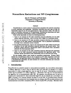
2.2. Mathematical Description of Mechanical Loads 2.2.1. Load Vector As described in the previous section, climatic loads induce in-plane and out-of-plane loads on photovoltaic modules. Figure 2 shows a photovoltaic module mounted at an inclination angle θ. Let us consider a load vector q (X1 , X2 ) acting at the outer surface O of the module in the following form. q (X1 , X2 ) = s (X1 , X2 ) + p (X1 , X2 )

187

188 189 190 191

192

(12)

with the in-plane load vector s (X1 , X2 ) = −sα (X1 , X2 ) eα and the out-of-plane load vector p (X1 , X2 ) = p (X1 , X2 ) n. 2.2.2. Direction of Loads This section focuses on the proper description of loads taking the inclination angle θ of a module into account. As a starting point, we introduce a fixed COOS gi as well as another COOS {ei } (with e3 ≡ n), which is connected to the photovoltaic module, cf. also Fig. 2. Considering a rotation around e2 by the angle θ, the following relations hold true g1 = cos (θ) e1 + sin (θ) e3

(13)

g2 = e2

(14)

g3 = − sin (θ) e1 + cos (θ) e3

(15)

or vice versa e1 = cos (θ) g1 − sin (θ) g3

193

(16)

e2 = g2

(17)

e3 = sin (θ) g1 + cos (θ) g3

(18)

The proper orthogonal tensor Q maps the basis gi onto the rotated basis {ei } such that Q can be represented as follows. Q = ei ⊗ gi

194

(19)

If one takes Eqs. (13)-(18) into account, one obtains the following representation for the rotation tensor. Q = Qi j ei ⊗ e j = Qi j gi ⊗ g j

195

(20)

with    cos (θ) 0 sin (θ)    1 0  Qi j =  0   − sin (θ) 0 cos (θ)

196 197

(21)

Next, we assume that a load vector a = ai gi is given with respect to the basis gi . The components a0i of the vector a = a0i ei with respect to the rotated basis {ei } are computed as follows, cf. [36] a0i = Q ji a j

198 199

200 201

(22)

In the following, above formulas are applied to loads resulting from natural weathering. We suppose that wind loads qW (X1 , X2 ) are horizontal, while snow loads qS (X1 , X2 ) refer to the vertical direction, cf. Fig. 2.    qW (X1 , X2 ) g1 , at wind loading qm (X1 , X2 ) =  ∀m = {W, S} (23)  qS (X1 , X2 ) g3 , at snow loading, where the amplitude functions qm (X1 , X2 ) need to be defined. With Eq. (22), one obtains the following representations for the load vectors.     qW (X1 , X2 ) cos (θ) e1 + qW (X1 , X2 ) sin (θ) n, at wind loading qm (X1 , X2 ) =  (24)  −qS (X1 , X2 ) sin (θ) e1 + qS (X1 , X2 ) cos (θ) n, at snow loading,

202

6

wind loading

snow loading

θ

Zo

qqSS

oM

qqW W θ e1

e1 θ e2 ≡gg2 g3

e1 θ e2 ≡gg2

g11 n

g3

n

e2

g11 n

Figure 2: Inclination angle θ with bases g1 , g2 , g3 and {e1 , e2 , n} for parametrisation of impact of snow and wind loads on a photovoltaic module

203 204 205 206

207 208

209 210 211 212

213

2.2.3. Amplitude and Spatial Distribution of Loads In order to analyse the influence of spatially heterogeneous loads, the load distribution with respect to gi is described by Eq. (23). In general, arbitrary amplitude functions qm (X1 , X2 ) can be taken into account by the finite element, which is presented in the next sections. As one example, this paper focuses on a double sine function. ! ! π π qm (X1 , X2 ) = q0m sin X1 sin X2 (25) L1 L2 Herein, q0m ∀m = {W, S} is the maximum amplitude. This concept can be easily generalised with a Fourier series to approximate experimental data which, however, is not available for the present study. ! ! k X k X πi πj qm (X1 , X2 ) = q0m sin X1 sin X2 ∀m = {W, S} ∧ k ∈ Z+ (26) ij L L 1 2 i=1 j=1 Due to the lack of experimental findings concerning distribution functions, this investigations are restricted to Fourier series with only one element (k = 1 ⇒ bi-harmonic distribution). The load constructed in Eq. (25) in context of the fixed COOS { gi } used in Eq. (23) must now be rotated into the photovoltaic module COOS {ei }. Considering Eqs. (24), the approximations for wind and snow loads result in the succeeding representations for the loading components. ! !  π π  0   s (X , X ) = −q cos(θ) sin X sin X  1 1 2 1 2 W   L1 L2  ! ! qW = −s1 e1 + pn with  (27)   π π  0   X1 sin X2  p(X1 , X2 ) = qW sin(θ) sin L1 L2 ! !  π π  0   X sin X sin(θ) sin s (X , X ) = q  1 2 1 1 2 S   L1 L2  ! ! qS = −s1 e1 + pn with  (28)   π π  0   X1 sin X2  p(X1 , X2 ) = qS cos(θ) sin L1 L2 Both loads can also be combined, what results in following expression for the total load qΣ . qΣ = qW + qS

(29) 7

214

215 216 217 218 219 220 221 222 223 224 225 226 227 228 229 230 231 232

3. Solution Approach with eXtended LayerWise Theory 3.1. Prerequisites In XLWT, all considerations are restricted to the mid surface S of the individual layers. The coordinates X1 , X2 describe points in the mid surface, which is transversally positioned at X3 = 0. Contemplations presented here are related to a planar mid surface, i.e. the structure is uncurved in the reference placement. It is equipped with a tripod COOS, while the unit vector perpendicular to the surface is called normal vector n. In-plane unit vectors are designated with {eα }. The surface boundary ∂S in these directions is indicated by the boundary normal ν. Therefore ν · n = 0 holds. The surface continuum is equipped with five DOF’s: two in-plane translational, one out-of-plane translational, and two out-of-plane rotational. These are in analogy with the kinematics suggested by Mindlin [2]. In-plane and out-of-plane loads sα and p can be applied. In-plane loads are applied to the outer surfaces O. Therefore, they act with a lever of ∓h/2, while h is the thickness of the layer. Due to line volatility of out-of-plane loads, they can be applied to the surface S directly. These assumptions are visualised in Fig. 3. For structural analysis of composite structures, an integer multiple of the described surface continuum is required. For XLWT, three (NK = 3) mid surfaces are coupled, as depicted in Fig. 4. We designate these surfaces with the superscript indices top (t), core (c), and bottom (b). All considerations are restricted to deformable plane surfaces, which are the mid planes (St , Sc , Sb ) of every individual layer. At the layer interfaces (It , Ib ), they are connected via constraints, kinematically and kinetically. All interacting forces act at these interfaces. External loading is applied at the outer surface O, while the back surface B remains unloaded. The following points have been assumed concerning the physical structure.

233

• Uniform thickness of the corresponding layers.

234

• Perfect connection of the layers at their interfaces. single layer mid surface continuum S ν

ϕ2 e1

s2

e2 n

p

u1

u2

h 2

s1

h 2

∂S

ν

ϕ1

w

mid surface S boundary ∂ S outer surface O

rotational degrees of freedom translational degrees of freedom loads

Figure 3: Mechanical model of a surface continuum S with boundary ∂S, COOS {e1 , e2 , n}, DOF’s u1 , u2 , w, ϕ1 , ϕ2 , and loads s1 , s2 , p

8

e1 three layered surface continuum

e2 e1

n

e2

O St It Sc

ht 2

Ib

ht 2

Sb

hc 2

B

hc 2 hb 2

mid surfaces St , Sc , Sb front surface O

interfaces It , Ib back surface B

hb 2

Figure 4: Composition of the three layered surface continuum with interfaces, outer surface, and distances to each other assigned

235

236

237 238

239 240

This leads to the subsequent properties for the surfaces. • All material points per surface continuum are coplanar in the reference placement. • All surfaces are plane-parallel in the reference placement and at constant distance to each other for any admissible placement. • Mid surfaces, interfaces, as well as outer front and back surfaces are kinematically coupled via the straight normal hypothesis of the Mindlin theory.

243

Specifications and consequences of these properties will be presented in the sequel, while we waive the derivation of the surface contiuum from 3D Cauchy continuum theory, given for example in [8] or [37] in detail, based on a projection of kinematic, kinetic, and constitutive quantities.

244

3.2. Degrees of Freedom

241 242

245 246 247 248 249 250 251

In order to determine the position of a material point on a surface, two components are completely sufficient so that x K = Xα eαK holds for every surface separately, while the superscript K = {t, c, b} is the layer index. Since we operate on single surfaces only, it is possible to divide the DOF’s into in-plane and out-of-plane measures. This is expressed by the in-plane displacements uαK and the deflections wK . Additionally, rotational DOF’s are introduced. While translational DOF’s possess components in all three spatial directions of the Euclidean space E3 , the rotational DOF’s possess out-of-plane components only, as introduced by Reissner [38]. This introduction of rotations is therewith contrary to that of Cosserat [39] or micropolar plates [40] for practical reasons, cf. [41]. The rotation about the normal to the 9

252

surface is not considered as independent variable. However, the DOF’s can thus be indicated as follows.   in-plane displacements: u K = uαK eα      K deflections: w n ∀ x K ∈ SK      out-of-plane rotations: ϕK = −ϕ2K e1 + ϕ1K e2 

253

Since we consider a three layered structure with K = {t, c, b}, a total of 15 DOF’s results at this point.

254

3.3. Kinematical Measures

255 256

(30)

Under the assumption that strains and curvatures remain small, linear kinematical measures are introduced based on the aforementioned DOF’s. membrane strains: EK = ∇sym u K K

sym K

curvatures: X = ∇

ϕ

K = Eαβ eα ⊗ eβ

=

transverse shear strains: γK = ∇wK + ϕK =

K χαβ eα γαK eα

(31) (32)

⊗ eβ

(33)

258

Herein, EK is the membrane strain tensor, X K is the curvature tensor, and γK is the transverse shear strain vector. The second rank tensors EK and X K are both symmetric.

259

3.4. Balance Equations and Kinetic Measures

257

260 261

262 263 264 265

The balance equations for the surface continuum, known as Euler’s first and second law of motion, are given as follows for every layer separately.    balance of momentum: ∇ · FK + fK =o  ∀ x K ∈ SK (34)   K K K  balance of moment of momentum: ∇ · M +F 1 +m =o Herin, FK is the force tensor (also known as force-stress tensor), FK 1 is the vectorial invariant of FK coupling both balance equations, M K is the axial tensor of moments (also known as moment-stress tensor), f K is the vector of interacting and external forces, and mK is the vector of interacting as well as external moments. The tensors FK and M K have the following properties, which are in analogy to Cauchy’s theorem. ν · FK = f νK K

ν· F = 266 267

mνK

n· FK = o

(35)

K

(36)

n· M = o

Here f νK and mνK are forces and moments at the boundary with normal ν. Force and moment tensor are both nonsymmetric. K K FK = Fαβ eα ⊗ eβ + Fα3 eα ⊗ n K

M = 268 269 270

K Mαβ eα

⊗ n × eβ =

K −Mαβ eα

(37) (38)

⊗ eβ × n

Since the force tensor is non-symmetric in general and distributed torques are not vanishing, the surface continum is considered as polar medium, even if the physical three dimensional structure of a photovoltaic module is non-polar, cf. [8]. The force tensor can be decomposed into a symmetric and a skew part. sym skw FK = FK + FK 1 K K > 1 K K > = F + F + F − F 2 2 = FK · P + FK · n ⊗ n =N

K

+

qKQ

(39a) (39b) (39c) (39d)

⊗n 10

K = Nαβ eα ⊗ eβ 271 272 273

K + Qα3 eα ⊗ n

(39e)

Herein, N K is the membrane force tensor, which is symmetric, and qKQ is the vector of transverse shear forces. Since K the second index in Qα3 is not varying, QαK is introduced here, what allows us to describe the shear force terms as a K vector qQ . qKQ = FK · n = QαK eα

274 275 276 277

278 279

(40)

The second rank tensor P = 1 − n ⊗ n used in Eq. (39c) is the perpendicular projector, cf. [42]. The vectorial invariant skw of the force tensor is determined by FK 1 = qKQ × n, so that FK = −1/2 FK 1 × 1 holds true. Figure 5 provides free-body diagrams for the individual layers of the three layered composite structure where stress resultants are depicted at positive edges. Concerning the interacting and external forces, the following relations can be deduced.    qt + p n + st − s if K = t     b  fK =  ∀ f K ∈ SK (41) q − qt n + sb − st if K = c      b b  q n− s if K = b In analogy to the decomposition of the force tensor FK , it is also possible to split f K additively into an in-plane f K and out-of-plane part f⊕K . f K = f K · (P + n ⊗ n) = f K · P + f K · n ⊗ n = f K + f⊕K n

280 281

(42)

The interacting as well as the external moments are determined by the following set of equations, where we restrict ourselves to moments generated by forces only.  t h t   if K = t  2 n× s + s    hc  K t b m = ∀ mK ∈ SK (43) if K = c  2 n× s + s    b   h n × sb if K = b 2

282 283 284

285

286 287

Variables used in Eqs. (41) and (43) are the in-plane interacting forces sK = sαK eα and the out-of-plane interacting forces qK . Inserting Relations (39)–(43) in Eqs. (34), we can determine the balances for the individual material surfaces of the composite structure. The balance of membrane forces takes the following form.    st − s if K = t     ∇ · N K + f K = o f K =  ∀ {sK , s} ∈ {IK , O} (44) sb − st if K = c     b −s if K = b The balance of transverse shear forces is indicated as follows.    qt + p if K = t     ∇ · qKQ + f⊕K = 0 f⊕K =  qb − qt if K = c      − qb if K = b

∀ {qK , p} ∈ {IK , O}

(45)

K Instead of the axial tensor of moments M K , the polar tensor of moments LK = Mαβ eα ⊗ eβ is introduced by the K K symmetrisation L = M × n. The balance of moment of momentum now reads as follows.  t h t   if K = t  2 (s + s )   c  K K K K h t b (46) ∇ · L − qQ + m × n = o m ×n= ∀ {sK , s} ∈ {IK , O}  2 (s + s ) if K = c   b  h b  s if K = b 2

11

Q Qt2t2

t

t N22

tt N N21 21

c N22

moments

St

St Q1t1 Q

tt N N12 12

1

tt N11 N 11

Sb 1

Qc1c1 Q

bb N N21 21

bb N N12 12

tt M12 M 12

t Mt11 M

t M21

cc N11 N 11

It

1 cc M12 12

cc M11 M 11

c M21

Ib

st2

st1

sst1t1

qt 1

sb2

Ib

1

b M12 M 12

b M11 M 11

b M21

st2

ssb1b1

qb sb1

1

bb M22 M 22

bb N11 N

s2

qqbb

Sb

Qb1b1 Q

It

p s1

qqtt

cc M M22 22

b b N22

O

Sc

cc c N21 N c12 N 21 N12

Q Qb2b2

external loading & interaction

tt M M22 22

Sc

Qc2c2 Q

c

forces

1

sb2

B 1

e2

e1 n

Figure 5: Stress resultants at mid surfaces (X3K = 0) as well as external and interacting forces at interfaces (X3 = ±hc/2), front (X3 = −hc/2 − ht ), and back surface (X3 = hc/2 + hb )

1 288 289 290

1

1

3.5. Constitutive Equations Considering a geometrically and physically linear theory, the constitutive equations for isotropic-homogeneous elastic 1 materials (material symmetry, invariance under rotations) can be formulated layerwise as linear mappings. membrane force - membrane strain relation: N K = C K : EK K

K

bending moment - curvature relation: L = D : X

K

transverse shear force - transverse shear strain relation: qKQ = Z K · γK 291 292 293 294 295 296 297

(47) (48) (49)

The measures C K , D K , and Z K used in Eq. (47), (48), and (49) are the fourth rank membrane stiffness tensor, the fourth rank bending stiffness tensor, and the second rank transverse shear stiffness tensor, respectively. As is apparent, coupling stiffnesses are not considered. This decoupling of membrane, bending and shear state, i.e. decoupling of stretching, bending, twisting, and shearing is legit since every single surface SK is halfway up between the nearest interfaces IK respectively front O or back surface B in both transverse directions (geometrical symmetry). This fact coincides with the assumption of a physical plane layer which is symmetric to its mid plane at X3K = 0. In the case of isotropic material behaviour, the constitutive tensors read as follows [4]. 1 − νK P1 + P2 2 1 − νK P1 + P2 = DBK νK P ⊗ P + DBK 2 = DSK P

K K K membrane stiffness tensor: C K = DM ν P ⊗ P + DM

bending stiffness tensor: D K transverse shear stiffness tensor: Z K

12

(50) (51) (52)

298 299

Here, E K , G K , and νK are the Young’s modulus, the shear modulus, and the Poisson’s ratio of the corresponding layer K material. The membrane rigidity DM , the bending rigidity DBK , and the shear rigidity DSK can be determined as follows. E K hK 1 − (νK )2 E K (hK )3 DBK = 12 1 − (νK )2 DSK = κ K G K hK

K DM =

300 301

(53a) (53b) (53c)

These representations are in accordance with classical thin-walled structural theories known from Kirchhoff [43], Reissner [44], and Mindlin [2]. P1 and P2 are fourth rank tensors.

P1 = eα ⊗ eβ ⊗ eβ ⊗ eα 302 303 304 305 306 307 308 309

310 311 312

3.6. Boundary Conditions With regard to the practical implementation of the balance equations, the definition of boundary conditions is inevitable. Hereby, we introduce homogeneous Dirichlet boundary conditions

315 316

317 318

∧∨ w(x K ) = 0

∧∨ ϕ(x K ) = o

∀ x K ∈ ∂SDK ,

∧∨ ν · LK = m?K

∧∨ ν · qKQ = q?K

∀ x K ∈ ∂SNK ,

3.7. Kinematical Constraints Following expression holds true (57)

since compression or dilatation in transverse direction is neglected, what results in equal deflections for all layers. wt = wc = wb = w

320 321 322

∀ x K = XαK eα

324

(58)

This stipulates that the reduced number of independent DOF’s for our composite is 13 at this point. As stated, we assume that all layers are rigidly connected at their interfaces for any admissible deformation process. The following kinematical constraints can therefore be deduced since the straight line hypothesis of Mindlin [2] is used. ht t hc ϕ = uc − ϕc (59a) 2 2 hb b hc ϕ = uc + ϕc (59b) ub − 2 2 Above constraints are used to substitute quantities of the core layer by the quantitites of the skin layers (t, b). As conseqence of Eqs. (59a) and (59b), the repeatedly reduced number of independent DOF’s is 9. ut +

323

(56)

whereby n?K , m?K , and q?K are membrane forces, moments, and transverse shear forces prescribed at the boundaries, while ∂SDK and ∂SNK denote Dirichlet and Neumann boundaries, respectively. Loads (in-plane s and out-of-plane p) at the outer surface of the top layer are implemented directly in the balance equations (44), (45), and (46).

∂hK ∂hK = =0 ∂X1 ∂X2 319

(55)

and Neumann boundary conditions which are built on Cauchy theorem, cf. Eqs. (35) and (36) , ν · N K = n?K

314

(54)

The stiffness tensors given in the compact representations (50), (51), and (52) are completely determined by two material parameters (E K , νK , when considering isotropic materials G K = E K/2(1 + νK ) holds true) and one geometry parameter (hK ), respectively, up to an undetermined parameter κ K , cf. Eq. (52). This so called shear correction factor is a parameter to set the shear energy contribution at deformation processes with shear soft layers. A value of κ K = 1 ∀ K = {t, c, b} is applied here since this setting showed best agreements with experimental validations, cf. [45]. κc= 1 is manifested by the fact, that shear stresses acting on It and Ib are contrary but equal in magnitude for transverse symmetric structures while the core layer is comparatively thin, what results in constant shear stresses along X3 with the limits ∓h/2. In contrast, κ K ∀ K = {t, b} is not decisive due to the high shear rigidity of these layers.

u(x K ) = o 313

P2 = eα ⊗ eβ ⊗ eα ⊗ eβ

13

325 326 327

3.8. Introduction of Mean and Relative Measures For the sake of brevity, mean (superscript ◦) and relative (superscript ∆) displacements and rotations are introduced, cf. [6, 8]. 1 t u − ub 2 1 t ∆ ϕ = ϕ − ϕb 2

1 t u + ub 2 1 t ◦ ϕ + ϕb ϕ = 2

u∆ =

u◦ =

328 329

(60b)

n o Considering Eqs. (60a) and (60b), the set of independent DOF’s is redefined as u◦1 , u◦2 , u∆1 , u∆2 , w, ϕ◦1 , ϕ◦2 , ϕ∆1 , ϕ∆2 . The corresponding membrane strain tensors, curvature tensors, and transverse shear strain vectors read as follows. E◦ = ∇sym u◦ = E∆ = ∇sym u∆ = X◦ = ∇sym ϕ◦ = X∆ = ∇sym ϕ∆ = γ◦ = ∇w + ϕ◦ = γ∆ = ϕ ∆

330

(60a)

=

1 t E + Eb 2 1 t E − Eb 2 1 t X + Xb 2 1 t X − Xb 2 1 t γ + γb 2 1 t γ − γb 2

(61a) (61b) (61c) (61d) (61e) (61f)

In addition, mean and relative stress resultants are defined. N◦ = Nt + Nc + Nb ∆

t

N =N −N

(62a)

b

(62b)

1 1 L◦ = Lt + Lc + Lb + hb + hc Nb − ht + hc Nt 2 2 L∆ = Lt − Lb q◦Q q∆Q 331

= =

qtQ qtQ

+ −

qcQ qbQ

+

(62c) (62d)

qbQ

(62e) (62f)

Constitutive equations with respect to the new stress resultants are formulated in analogy to Eqs. (47), (48), and (49). N◦ = C ◦ : E◦ + C ∆ : E∆ + C c : Ec ∆

∆

(63a)

∆

◦

N =C :E +C :E ◦

◦

∆

(63b) c

∆

c

L =D :X +D :X +D :X i 1h − h∆ C ◦ + (hc + h◦ ) C ∆ : E◦ 2 i 1h − (hc + h◦ ) C ◦ + h∆ C ∆ : E∆ 2 ∆ L = D ∆ : X◦ + D ◦ : X∆ ◦

q◦Q q∆Q 332

◦

∆

∆

c

= Z ·γ +Z ·γ +Z ·γ ◦

◦

∆

◦

= Z ·γ +Z ·γ ◦

(63c) (63d)

c

(63e)

∆

(63f)

In above equations, new stiffness tensors have been introduced.

C◦ = Ct + Cb

C∆ = Ct − Cb

(64a) 14

D∆ = Dt − Db

D◦ = Dt + Db Z 333

◦

t

=Z +Z

b

Z

∆

t

=Z −Z

(64b)

b

(64c)

Furthermore, new thickness measures are defined. h◦ =

1 t h + hb 2

h∆ =

1 t h − hb 2

(65)

334 335

336 337 338 339 340 341 342 343 344

3.9. Principle of Virtual Work As basis for the numerical implementation, this section presents the principle of virtual work for the XLWT. The principle of virtual work is applied to the XLWT in the usual way, cf. also [6, 46, 47]. In a first step, the balance equations are combined with the corresponding virtual DOF’s, i.e. Eqs. (44) are multiplied with the virtual in-plane displacements, Eqs. (45) are multiplied with the virtual deflections, and Eqs. (46) are multiplied with the virtual cross-section rotations. All balance equations are summed up and integrated over the surface. One introduces the mean and relative measures from the previous subsection and uses the kinematical constraints in order to replace the DOF’s of the core layer by the mean and relative DOF’s. After considering the constitutive equations, one obtains the following expressions for the internal and external work. Z δWint = δE◦ : C ◦ : E◦ + δE∆ : C ◦ : E∆ + δE◦ : C ∆ : E∆ S

! 1 ∆ ◦ 1 ◦ ∆ + δE : C : E + δE + h δX + h δX : C c 2 2 ! 1 1 : E◦ + h∆ X◦ + h◦ X∆ + δγ◦ · Z ◦ · γ◦ 2 2 ∆

∆

◦

◦

+ δγ∆ · Z ◦ · γ∆ + δγ◦ · Z ∆ · γ∆ + δγ∆ · Z ◦ · γ◦ " # 1 ◦ ∆ c ◦ ◦ ∆ ∆ + δγ − c 2δu + (h + h ) δϕ + h δϕ · Z c h " # 1 ∆ c ◦ ◦ ∆ ∆ ◦ · γ − c 2u + (h + h ) ϕ + h ϕ h

δWext

+ δX◦ : D ◦ : X◦ + δX∆ : D ◦ : X∆ + δX◦ : D ∆ : X∆ 1 + δX∆ : D ∆ : X◦ + 2δE∆ + h◦ δX◦ + h∆ δX∆ : D c 2 c (h ) ∆ ◦ ◦ ∆ ∆ : 2E + h X + h X dS " ! # Z 1 1 = δu◦ + h∆ δϕ◦ · n◦ν + δu∆ + (hc + h◦ ) δϕ◦ · n∆ν 2 2

(66)

∂Sp

1 + h◦ δϕ∆ · ncν + δwq◦ν + δϕ◦ · m◦ν + δϕ∆ · m∆ν 2 i 1 h − c 2δu∆ + (hc + h◦ ) δϕ◦ + h∆ δϕ∆ · mcν d ∂Sp h Z " t h + δϕ◦ + δϕ∆ · s − δu◦ + δu∆ · s 2 Sp

# + δwp d Sp

(67) 15

345 346

Hereby, Sp and ∂Sp denote the surface and boundary of the continuum, where boundary conditions with respect to the stress resultants are prescribed  NpK = N K ∂S    p     K K Lp = L ∂S  ∀ K = {◦, ∆, c} (68)   p       qKQp = qKQ ∂S p

347

348 349

Furthermore, stress resultants on the boundary of the surface continuum have been introduced.  nνK = ν · NpK       K K mν = ν · Lp  ∀ K = {◦, ∆, c}     K K  qν = ν · qQp

Equations (66) and (67) are inserted into the principle of virtual work, which states that the balance equations of a body are fulfilled if the virtual work of the internal forces equals the virtual work of the external forces [47]. δWint = δWext

350

351 352 353 354 355 356 357 358

(69)

(70)

4. Numerical Implementation 4.1. Basic Procedure in Finite Element Method Typically, quadrilateral finite elements are used to model thin-walled structures with single layer, while for structures with NK> 1 different approaches exist, cf. [7, 48]. The main idea of the present work is to represent all layers with one element in transverse direction. While in [6] a complete description of this approach with finite elements is given, the principles of numerical solution strategy are presented here. The FEM is based on a strict separation of structural and element scales. The whole two dimensional domain Ω is divided into subdomains Ωe , i.e. the finite elements. Thereby, the domain Ω comprises the subdomains Ωe , which must not overlap. Ω=

NE [

Ωe

Ωi ∩ Ω j = ∅

if i , j

(71)

e=1 359 360

NE is the number of elements in the domain Ω. The principle of virtual work has to be fulfilled on the whole domain Ω, cf. also Eq. (70), and on each subdomain Ωe e e δWint = δWext ,

361

while the virtual work of the structure is obtained by adding the virtual work of all finite elements. δWint =

NE X e=1

362 363 364 365 366

367

(72)

e δWint

δWext =

NE X

e δWext

(73)

e=1

4.2. Shape Functions Since the exact values of the DOF’s on the domain Ω and on the subdomains Ωe are unknown, one uses the shape functions N i in order to approximate the solution. For the finite layerwise element, SERENDIPITY type shape functions are applied, cf. also Fig. 6. The shape functions are defined with respect to the natural coordinates −1 ≤ ξ j ≤ 1, ∀ j = {1, 2} [49, 50]. i ih ih 1h N i (ξ) = 1 + ξ1i ξ1 1 + ξ2i ξ2 ξ1i ξ1 + ξ2i ξ2 − 1 i = {1, . . . , 4} 4 ih i 1h N i (ξ) = 1 + ξ1i ξ1 1 − ξ22 i = {6, 8} 2 ih i 1h N i (ξ) = 1 + ξ2i ξ2 1 − ξ12 i = {5, 7} 2 The index i represents the node number, while the node numbering is depicted in the centre of Fig. 6. 16

N8

N4

N7

ξ2

ξ2

ξ2

ξ1

ξ1

ξ1

N1

element patch

N3 7

8

ξ2

ξ1

4

1 5

6

ξ2

ξ1

ξ2 3

ξ1

2 N5

N2

N6

ξ2

ξ2

ξ2

ξ1

ξ1

ξ1

Figure 6: Approximation of deformations with SERENDIPITY type shape functions of quadratic order of interpolation

368

369 370 371

4.3. Jacobi Transformation The transformation of differential line elements dXi and dξi is based on the derivatives of the physical coordinates with respect to the natural coordinates. This transformation is performed via the Jacobi matrix J(ξ) and its inverse J(ξ)−1 . In two dimensions, it holds true [51] ∂ ∂ = J(ξ) ∂ξ ∂x

372

374

∂ ∂ = J(ξ)−1 ∂x ∂ξ

(74)

with  ∂X  1  ∂ξ1 J(ξ) =   ∂X1  ∂ξ2 " ∂ ∂ = ∂ξ1 ∂ξ

373

⇔

∂X2   ∂ξ1   ∂X2   ∂ξ2 #> ∂ ∂ξ2

 ∂X 2  1  ∂ξ2 −1 J(ξ) =  |J(ξ)|  ∂X1 − ∂ξ2 " #> ∂ ∂ ∂ = . ∂x ∂X1 ∂X2

∂X2   ∂ξ1   ∂X1   ∂ξ1

−

(75)

(76)

The determinant of the Jacobi matrix det[J(ξ)] = |J(ξ)| is utilised to transform an infinitesimal surface element dΩ in physical coordinates into an infinitesimal surface element in natural coordinates. dΩ = dX1 dX2 = |J(ξ)| dξ1 dξ2

(77) 17

375 376 377 378

379 380

381 382

383

384

4.4. Discretisation 4.4.1. Degrees of Freedom In order to discretise equations, the vector of DOF’s at every node i is specified as follows (recall DOF definitions of sections 3.7 and 3.8). h i i i i i i i i i > ai = u◦1 u◦2 u∆1 u∆2 wi ϕ◦1 ϕ◦2 ϕ∆1 ϕ∆2 ∀ i = {1, . . . , NN} (78) while NN = 8 is the number of nodes per element. All nodal vectors of DOF’s are assembled to the element vector of DOF’s referring to the nodal values of DOF’s. h i> ae = a1 a2 . . . aNN (79) In order to obtain the fields of DOF’s over the element with respect to the natural coordinates ξ, the DOF’s are interpolated into the shape functions, applying the isoparametric element concept. h i> a (ξ) = u◦1 (ξ) u◦2 (ξ) u∆1 (ξ) u∆2 (ξ) w (ξ) ϕ◦1 (ξ) ϕ◦2 (ξ) ϕ∆1 (ξ) ϕ∆2 (ξ) ≈ N (ξ) ae (80) with the matrix of shape functions N (ξ) h i N (ξ) = N1 (ξ) N2 (ξ) . . . NNN (ξ)

(81)

and the matrix of shape functions at node i Ni (ξ) = N i (ξ) I ,

385

386 387 388

389

390 391 392 393

while I is a quadratic identity matrix, whose number of columns and rows is equal to the number of DOF’s per node. 4.4.2. Kinematical Measures As a next step, the kinematical equations, cf. also Eqs (61), are discretised. For this purpose, we introduce kinematical vectors with respect to the element. h i> h i> eMB = e◦M e∆M e◦B e∆B eS = e◦S e∆S (83) with the auxiliary vectors for membrane and transverse strains as well as curvatures i h i> h ◦ ◦ > ◦ E22 2E12 e◦M = E11 = u◦1,1 u◦2,2 u◦1,2 + u◦2,1 h i h i> ∆ ∆ ∆ > E22 2E12 = u∆1,1 u∆2,2 u∆1,2 + u∆2,1 e∆M = E11 i> h i> h e◦B = χ◦11 χ◦22 2χ◦12 = ϕ◦1,1 ϕ◦2,2 ϕ◦1,2 + ϕ◦2,1 h i> h i> = ϕ∆1,1 ϕ∆2,2 ϕ∆1,2 + ϕ∆2,1 e∆B = χ∆11 χ∆22 2χ∆12 i> h i> h = w,1 + ϕ◦1 w,2 + ϕ◦2 e◦S = γ1◦ γ2◦ h i> h i> e∆S = γ1∆ γ2∆ = ϕ∆1 ϕ∆2

(84) (85) (86) (87) (88) (89)

Please note that above kinematical vectors represent fields, i.e. these vectors depend on the natural coordinates ξ. For the sake of brevity, this has not been written explicitly. Now, the kinematical fields are approximated in analogy to Eq. (80) by introducing the strain matrices BMB and BS for the membrane and bending as well as for the shear part, respectively. eMB (ξ) ≈ BMB (ξ) ae

394

(82)

eS (ξ) ≈ BS (ξ) ae

(90)

The kinematical matrices are the products of the differential operators D and the matrix of shape functions N. BMB (ξ) = DMB N (ξ)

BS (ξ) = DS N (ξ)

(91) 18

395

with the differential operators for membrane, bending, and shear state h

DMB = D◦M

h DS = D◦S 396

399 400 401

0 0 0 0 0 0 0 0 0 0 0 0 0

(93)

 0 0 0 0 0 0 0  ∂ 0 0 0 0 0 0 0 ∂X2  ∂ 0 0 0 0 0 0 0 ∂X1  ∂ 0 0 0 0 0 0 ∂X1  ∂ 0 0 0 0 0 0 ∂X2  ∂ ∂ 0 0 0 0 0 ∂X2 ∂X1  0 0 0 ∂X∂ 1 0 0 0  ∂ 0 0 0 0 0 0 ∂X2  0 0 0 ∂X∂ 2 ∂X∂ 1 0 0  0 0 0 0 0 ∂X∂ 1 0   ∂  0 0 0 0 0 0  ∂X2  ∂ ∂  0 0 0 0 0 ∂X2 ∂X1 # 0 0 ∂X∂ 1 1 0 0 0 0 0 ∂X∂ 2 0 1 0 0 # 0 0 0 0 0 1 0 . 0 0 0 0 0 0 1

(94)

(95)

(96)

(97)

(98) (99)

In order to implement the finite element, the expressions for the virtual internal and external work, cf. Eqs. (66) and (67), need to be transferred to a matrix notation, what is discussed in the next section. For this reason, this section presents the corresponding constitutive equations in a matrix notation. First, vectors for the stress resultants are introduced in analogy to Eqs. (84)-(89). h

sSK = Q1K

h

K sBK = M11

h

403

(92)

i>

4.5. Constitutive Equations for FEM

K K sM = N11

402

i>

0

∂X2

 0  D∆M = 0  0  0  D◦B = 0  0  0  D∆B = 0  0 " 0 D◦S = 0 " 0 D∆S = 0

398

D∆S

D∆B

D◦B

and the auxiliary differential operators  ∂  ∂X1  D◦M =  0  ∂

397

D∆M

K K N22 N12 i> Q2K K M22

i>

K M12

i>

∀ K = {◦, ∆, c}

(100)

∀ K = {◦, ∆, c}

(101)

∀ K = {◦, ∆, c}

(102)

Now, the constitutive equations are reformulated in a matrix notation, while Eqs. (63) serve as basis for the mean and relative variables, and Eqs. (47), (48), and (49) are evaluated for the core layer. ˆ◦ +C ˆ c e◦ + C ˆ ∆ e∆ + 1 C ˆ c h∆ e◦ + h◦ e∆ s◦M = C B B M M M M M M

(103)

ˆ ◦ e∆ + C ˆ ∆ e◦ s∆M = C M M M M

(104)

2

" # 1 ∆ ◦ c c ◦ ◦ ∆ ˆ sM = CM eM + h eB + h eB 2 ˆ ◦ e◦ + C ˆ ∆ e∆ + C ˆ c e◦ + A1 a s◦ = C S

S S

S S

S

(105) (106)

S

ˆ ◦ e∆ + C ˆ ∆ e◦ s∆S = C S S S S scS

=

ˆc C S

e◦S

+ A1 a

(107)

(108) 19

1 ˆc ∆ ◦ ◦ ∆ ∆ C 2 e + h e + h e M B B B hc i 1 ˆ◦ h ∆ ◦ − CM h eM + (hc + h◦ ) e∆M 2 i 1 ˆ∆ h ∆ ∆ c ◦ ◦ − C M h eM + (h + h ) eM 2 ∆ ˆ ◦ e∆ + C ˆ ∆ e◦ sB = C B B B B 1 ˆ c 2e∆ + h◦ e◦ + h∆ e∆ scB = − c C M B B B h

ˆ ◦ e◦ + C ˆ ∆ e∆ − s◦B = C B B B B

(109) (110) (111)

404

ˆK, C ˆ K, C ˆ K ∀ K = {◦, ∆, c} as well as the auxiliary matrix A1 are defined in the appendix. The constitutive matrices C M S B

405

4.6. Element Stiffness Relation

406 407 408 409

This section derives the element stiffness relation based on the principle of virtual work. As a first step, the virtual internal and external work are presented in a matrix notation. First, Eq. (66) is transferred to a matrix notation considering the vectors of strains and stress resultants as well as the constitutive relations introduced in Sections 4.4.2 and 4.5. Then, Eqs. (80) and (90) are inserted such that one obtains Z h > ˆ c A2 BS δWint = δae> B>S C◦S + C∆S + C∆S + A>2 C S Ωe

> ˆ c A1 N + B> A> C ˆc ˆ c A1 N + B>S A>2 C + N> A>1 C S 2 S A1 N S S ˆ c A3 + B>MB C◦MB + C∆MB + C∆MB + A>3 C M i ˆ c A4 BMB ae dΩe + A>4 C B >

410 411 412 413

The introduced auxiliary matrices Ai ∀ i = {1, . . . , 5} are defined in the appendix. In order to shorten above expression, the generalised constitutive matrices C◦MB , C∆MB , C◦S , and C∆S have been introduced. Their definitions can be found in the appendix, too. Furthermore, all integrals are performed with respect to the element surface Ωe or the element boundary ∂Ωe , respectively. Now, Eq. (67) is proceeded similarly, what results in the following expression Z Z e> > e δWext = δa N A5 t d ∂Ωp + δae> N> q dΩe (113) ∂Ωep

414

415 416 417

418 419

(112)

Ωe

The vectors t and q contain loads that are distributed over a curve or a surface of the plate, respectively. h i> t = n◦ν n∆ν ncν q◦ν m◦ν m∆ν mcν h i> t t t t q = −s1 −s2 −s1 −s2 p h2 s1 h2 s2 h2 s1 h2 s2

(114) (115)

The vectors n◦ν , n∆ν , ncν , m◦ν , m∆ν , and mcν refer to the corresponding vectors in tensor notation defined in Eq. (69). In order to derive the element stiffness relation, Eqs. (112) and (113) are inserted into Eq. (70), and coefficients are equated with respect to the vector δae> . This yields the element stiffness relation KeMB + KeS ae = re (116) Hence, the stiffness matrix for the membrane and bending state KeMB and the stiffness matrix for the shear state KeS are determined as follows. Z ◦ ∆ ∆ > >ˆc KeMB = B> MB CMB + CMB + CMB + A3 CM A3 Ωe

ˆ c A4 BMB dΩe + A>4 C B

(117) 20

Z " ◦ ∆ ∆> >ˆc B> S CS + CS + CS + A2 CS A2 BS

KeS =

Ωe

> ˆc ˆ c A1 N + B> A> C + B>S A>2 C S 2 S A1 N S # ˆ c A1 N dΩe + N> A>1 C S 420

(118)

The right-hand-side vector re comprises all the line loads re1 and the surface loads re2 on the element. re = re1 + re2

421

(119)

with re1 =

Z

N> A5 t d ∂Ωep

re2 =

423 424

425

426 427

428

N> q dΩep

(120)

Ωep

∂Ωep 422

Z

4.7. Surface Load Vector Since this paper aims to analyse surface loads on photovoltaic modules, we focus on the surface load vector re2 . For the numerical procedure, the load vector q is approximated via the isoparametric element concept, in analogy to Eq. (80). q (ξ) ≈ N (ξ) qe

(121)

with the element load vector qe , which comprises all nodal load vectors qi h i> qe = q1 q2 . . . qNN i> h t t t t qi = −si1 −si2 −si1 −si2 pi h2 si1 h2 si2 h2 si1 h2 si2

(122) (123)

i i i The variables s1 , s2, and p are determined by evaluating the load distribution functions at the corresponding node i i coordinates X1 , X2 . si1 = s1 X1i , X2i si2 = s2 X1i , X2i pi = p X1i , X2i (124)

Equation (121) is inserted into Eq. (120) such that the surface load vector is approximated as follows. Z e r2 ≈ N (ξ)> N (ξ) qe dΩep

(125)

Ωep 429 430 431 432 433 434 435

4.8. Ensembling In order to obtain numerical equations for the whole structure, the virtual energies of all finite elements belonging to the structure, i.e. e ∈ [1, NE], are summed up, considering the relations between the DOF’s of every element and structural DOF’s. This procedure transfers variables on elemental scale to the structure. Based on the displacement vectors, stiffness matrices, and right-hand-side vectors of the element, one obtains the corresponding structural vectors and matrices. S The symbolic operator is used to ensemble the finite elements [50]. KMB =

NE [

KeMB

KS =

e=1

a

=

NE [ e=1

436

NE [

KeS

(126)

re

(127)

e=1

ae

r

=

NE [ e=1

Finally, the structural stiffness relation is formulated. Ka = r

(128) 21

437

The structural stiffness matrix is composed by a membrane-bending KMB and a shear portion KS . K = KMB + KS .

438 439 440 441 442

4.9. Numerical Integration and Artificial Stiffening Effects To determine the stiffness matrices and load vectors, it is necessary to calculate integrals over the element surface. The method to solve these integrations numerically used here is the so called Gauss-Legendre quadrature [50], which is established in FEM. In order to solve the exact analytical integration I of a function f (ξ) over the element surface, Eq. (77) is used: I=

Z

e

f (ξ) dΩ =

Ωe 443

446

f (ξ) |J(ξ)| dξ1 dξ2

(130)

−1 −1

NG1 X NG2 X i=1 j=1

445

Z1 Z1

The integral is approximated by the weighted summation of function values [52]. I≈

444

(129)

αi1 α2j f (ξ1i , ξ2j )

(131)

The function to be integrated is evaluated at the integration or Gauss points ξ1i , ξ2i and multiplied with the weighting factors αi1 , αi2 , while NG is the number of integration points. The position of the integration points is shown in Fig. 7 at the SERENDIPITY element.

447 448 449 450 451 452 453 454 455

Typical problems with finite elements are related to artificial stiffening effects. The probably best known phenomenon of this kind is the so-called shear locking. This stiffening effect becomes particularly relevant when bending states at slender structures are under investigation [53]. In that case, the shear rigidity is parasitic. Due to that, in addition to complete integration, two additional modes of integration are introduced to prevent shear locking [54]. The modes providing a remedy are the reduced and the selective integration. In this case, a reduced number of Gauss points is addressed for integration, or a reduced or the complete number of Gauss points is selected according to the rigidity portion. The principle procedures of all three integration modes are explained in Fig. 7, while coordinates of Gauss points and corresponding weights for complete and reduced integration are given in Table 1. Table 1: Coordinates of Gauss points und assigned weights of Gauss-Legendre quadrature [52]

m×m

ξ11 = − 3×3

ξ2j

ξ1i q

3 5

ξ12 = 0 ξ13 = +

ξ21 = −

αi , α j q

3 5

ξ22 = 0 q

3 5

ξ23 = +

q

3 5

α1 =

5 9

α2 =

8 9

α3 =

5 9

ξ11 = − √13

ξ21 = − √13

α1 = 1

ξ12 = + √13

ξ22 = + √13

α2 = 1

2×2

22

full

reduced

3×3

2×2

× – membrane

3×3

× – shear

2×2

ξ2

ξ2

ξ2

ξ1

ξ1

ξ1

× – membrane part

× – bending

selective

× – membrane part

× – bending × – shear

× – bending

part

× – shear × – G AUSS points – nodes

description:

Figure 7: Implemented integration modes for SERENDIPITY element with quadratic shape functions: full, reduced, and selective integration

456

5. Structural Analysis

457

5.1. Test Structure

458 459 460 461 462 463 464 465 466 467 468

As also done in different studies [6, 8], a commercial, 72 cell photovoltaic module with glass front and back cover and ethylene-vinyl acetate (EVA) as core layer material is used for the case studies in the present contribution. Nevertheless, there is a large variation of possible geometries and materials at the market, as reported in [8]. However, lengths and thicknesses used here are exemplaric. Geometrical measures used for this study are presented in Table 2. Hence, a length ratio LR = L2/L1 = 0.5 results. For the sake of simplicity, a structure, whose geometrical and material properties are symmetric in transverse direction, is used. The thickness ratio is TR = hc/(ht + hb ) ≈ 15.6 · 10−2 , and the thickness-to-length ratio is TLR = H/Lmin = 9.1 · 10−3 . Material parameters at room temperature (23◦ C) of the photovoltaic module under consideration are also given in Table 2, where isotropic elastic material behaviour is assumed. Glasses for the skin layers are stiff brittle materials, while the EVA for the core layer is a soft rubber-like material. Due to the extreme differences in material properties, the shear modulus ratio is GR = Gc/G s = 9.98 · 10−5 ∀ s = {t, b}, and the normalised shear rigidity parameter is β = 9.40 according to [4]. While GR confirms that classical composite theories cannot be Table 2: Geometrical and material parameters of the test structure used for convergence analysis (room temperature ϑ = 23◦ C)

K t/b

L1K [mm]

L2K [mm]

1620

810

hK [mm]

E K [N/mm2 ]

νK [−]

3.2

73.0 · 103 [55]

0.30 [55]

1.0

7.9 [56]

0.41 [56]

c 23

Table 3: Definition of boundaries at the layerwise structure and chosen boundary conditions for convergence study (H =

P

hK )

boundary

Γ11

Γ21

Γ12

Γ22

ΓN

e1

0

L1

0 . . . L1

0 . . . L1

0 . . . L1

e2

0 . . . L2

0 . . . L2

0

L2

0 . . . L2

n

−H/2 . . . H/2

−H/2 . . . H/2

−H/2 . . . H/2

−H/2 . . . H/2

−H/2

condition

w=0

w=0

w=0

w=0

qW = 500 N/mm2

u1K = 0

471 472 473 474 475 476 477 478 479 480

481 482 483 484 485 486 487 488 489

applied here due to the highly differing material properties, the shear rigidity parameter indicates the application range of XLWT. Compared to studies presented in [4, 5, 6, 8], β with respect to room temperature is in the range, where the first order shear deformation theory is also applicable to obtain useful results. Since the aim of this study is also the consideration of realistic temperatures at loading, β will vary such that the necessity of XLWT will be shown in the sequel. For the mounting of a photovoltaic module, a peripheral frame surrounding the composite structure as shown in [8] is considered here. Since it is already shown in [57, 58] that framing all-round the photovoltaic composite is favourable due to lower mechanical stresses compared to mounting at specific points at the sides along Lα , this concept is also applied here. It is assumed that the bedding material in the groove of the frame can transmit pressure, but not tension. In the absence of data on the compliance of the bedding material, an elastic bedding is renounced here. For a clear definition of the mounting, the boundaries Γβα are introduced in Table 3. Additionally, the boundary ΓN is defined as loaded area at the photovoltaic module. 5.2. Discretisation and Convergence For verification of the numerical implementation of XLWT, a convergence study is conducted here via discretisation variation. Used boundary conditions are given in Table 3. A constant wind load is applied to the outer surface of the photovoltaic module under inclination angle of 35◦ such that the loading is uniform, but non-orthogonal. This loading scenario corresponds to an orthogonal portion with p = 409.58 N/mm2 and a transverse portion of s1 = 286.79 N/mm2 , where Eq. (24) holds true for the component notation at ΓN . The spatial discretisation of the structure presented in the previous section is done via the finite element described in Section 4.4. A structured mesh is used, where all interior angles of the finite elements account for 90◦ . The discretisation density has been varied within a convergence study by changes of the element edge lengths. As can be 1.0

NE = 8, 192

full selective reduced

0.8

9.20

0.6

full selective reduced

9.15 9.08

0.4

·10−1

ZOOM

9.07

0.2 0.0

·10−1

wmax [mm]

470

w [mm]

469

9.10

9.06 9.05 0.48

0

0.2

0.50

0.4

0.52

X˘10.6 [−]

0.54

0.8

9.05

1

0 512

2,048

4,096

NE [−]

8,192

Figure 8: Discretisation variation through he adaption: deflection path along plate bisecting line and convergence of maximum deflection

24

1

Table 4: Characteristic parameters of the discretisation variation resulting through heα adaptation at the composite structure

mesh

1

2

3

4

NE

128

512

2,048

8,192

NN

433

1,633

6,337

24,961

NEQ

3,897

14,697

57,033

224,649

full

2,304

4,608

18,432

73,728

red.

1,024

2,048

8,192

32,768

1

1

1

1

NG

AR

512

seen in Table 4, the aspect ratio of the finite elements is kept constant at AR = hemax/hemin = 1 for all discretisation variations, i.e. he1 = he2 ∀ Ωe ⊂ Ω holds true. Therein, heα is the element edge length. Furthermore, NN = NE ×NNE is the number of nodes and NEQ is the total number of degrees of freedom (NEQ = NN ×NDOF) in corresponding discretised domain, where NNE is the number of nodes per element (8 in present case) and NDOF is the number of degrees of freedoms per node (9), while NE is the total number of elements. Considering the number of integration points (NG) given in Table 4, we distinguish between full and reduced (red.) integration scheme according to Fig. 7 resulting from Section 4.9. In summary, three integration schemes at four discretisation variants are used for the convergence study. Results of the convergence analysis are shown in Fig. 8. On the left-hand side, the deflection is depicted along a path representing the bisecting line of the plate. X˘ 1 = X1/L1 is a normalised measure. On the right-hand side, the maximum deflection of the plate versus the number of elements is given. It is conspicuous that it is sufficient to calculate with a maximum of 8, 192 elements in the present case, compared to conventional structural analysis with 3D elements, where 106 to 108 elements are needed to gain convergence [59]. By varying the number of elements, it is found that selective integration provides fastest convergence. Maximum calculation times were clearly below one minute for the highest disretisation density, while all simulations were performed on an eight core Intel i7-5960X CPU and 64 GB RAM by using the solver of ABAQUS 6.14. It should be noted that deflections decrease with increasing number of elements applying the reduced integration scheme, which seems unphysical. However, this phenomenon is shown in [6] also and will not be discussed here. As is apparent, the deformation field along X˘ 1 is unsymmetric (see magnification in left plot of Fig. 8) due to the non-orthogonal loading. For the maximum element number used here, reduced integration results in the largest deflections, while full integration leads to the stiffening of the elements. However, difference in the maximum deflection of all three integration schemes is around 10−3 mm, while the maximum deflection is 9.08 · 10−1 mm. In the sequel, all calculations are performed by using 8, 192 elements, where the selective integration is favoured since this scheme seems to be insensitive to artificial stiffening, also at low discretisation densities.

513

5.3. Case Studies

490 491 492 493 494 495 496 497 498 499 500 501 502 503 504 505 506 507 508 509 510 511

514 515 516 517 518 519 520 521 522 523

As already mentioned, snow loads act at sub-zero temperatures. In contrast, wind loads are independent of temperature. Due to the lack of data for material parameters of the core layer at any admissible temperature with respect to the range of application, cf. [8], these case studies are restricted to snow loading at −40◦ C and to wind loading at +80◦ C as two extrema. In contrast to the temperature dependent material behaviour of the core layer, we assume that the material parameters of the skin layers made of glass are insensitive with respect to temperature changes. Temperature dependent material parameters of the core layer for both case studies are given in Table 5. The high value of β = 106.74 at decreased temperatures indicates that also the Kirchhoff theory can be used. Contrary to that, β = 2.41 at elevated temperatures requires the XLWT [4, 5, 6]. This behaviour is also confirmed by the shear modulus ratio GR. Boundary conditions for edge support and loading at the front surface are given in Table 6 for snow and wind load. In both cases, the load distribution at ΓN is assumed to be well described by a double sine function with respect to COOS 25

Table 5: Temperature dependent material parameters of core layer material (based on [56])

524 525 526 527

ϑ [◦ C]

E c [N/mm2 ]

νc [−]

Gc [N/mm2 ]

GR [−]

β [−]

−40

1019.04

0.41

361.36

1.29 · 10−2

106.74

+80

0.52

0.41

0.18

6.57 · 10−6

2.41

{ gi } as given in Eq. (25). This double sine function is rotated in the COOS {ei } by the angle θ using Eqs. (27) or (28). For both load cases, the angle is varied, i.e. θ = {25◦ , 35◦ , 45◦ , 55◦ }. Compared to load intensities in natural weathering discussed in Section 2.1, the loads used here are kept small since just the procedure is in the foreground. At both cases, the maximum amplitude of loading is 500 N/mm2 .

528 529 530 531 532 533 534 535 536 537 538 539

540 541 542 543 544 545 546 547 548 549 550 551 552 553 554 555 556

Since the transverse loads of both loading scenarios act opposite when considering the loaded surface inclined with 0 < θ < 90◦ , different boundary conditions for the photovoltaic composite are needed at Γ11 and Γ21 . These are presented in Table 6. In the sequel, the evaluations are divided in two case studies. Figures 9 and 10 show the DOF’s for all layers along two paths with respect to a varying inclination angle. The paths are A-A (X1 = 0 . . . L1 , X2 = L2/2) and B-B (X1 = L1/2, X2 = 0 . . . L2 ), while normalised length measures X˘ α = Xα/Lα are used. In addition, kinetic and kinematical quantities for the individual layers are juxtaposed comparatively in Figs. 11, 12, 13, and 14, while only an inclination angle of θ = 35◦ is taken into account for the sake of clarity. This value represents a typical average for modules mounted in the area of Germany (around 47◦ . . . 52◦ of latitude) [60] since the optimum setting is always perpendicular to the sun. Due to the K K K symmetry of the second rank tensors N K, LK, EK and X K, the evaluation is restricted to the elements 11 , 22 , and 12 ∀ = {N, M, E, χ}. All results are discussed in Section 5.4. 5.4. Results and Discussion 5.4.1. Degrees of Freedom Figure 9 displays the deflection, the in-plane displacements, and the rotations along the Paths A-A and B-B for wind loading at elevated temperatures. It becomes obvious that the deflection increases with growing inclination angle. In contrast to pure orthogonal loading, cf. [8, 6], the deflection is non-symmetric due to the introduction of tangential loads. The maximum deflection is not located at the plate centre anymore, i.e. wmax , w(L1/2, L2/2), and equals wmax ≈ 1.95 mm for θ = 55◦ . The displacement u1K approaches its extremum near the edge X˘ 1 = 0, while u1K (X˘ 1 = 1) = 0 holds true due to the boundary conditions in Table 6. The absolute displacement |u2K | is equal in top and core layer along the Path B-B with opposite signs and the displacement in the core layer tends to zero. Contrarily, the rotations ϕ1K and ϕ2K are equal in the skin layers, while the core layer rotates in opposite direction. For comparison, Figure 10 displays the deflection, the in-plane displacements, and the rotations along the Paths A-A and B-B for snow loading at reduced temperatures. Contrary to wind loading, the deflection increases with decreasing inclination angle, such that the maximum deflection occurs at θ = 25◦ and equals wmax ≈ 0.45 mm. At X˘ 1 = 0, the derivative of the deflection with respect to X˘ 1 tends to zero. This is due to the constrained displacements u1K . Subsequently, the mutual sliding between the skin layers is decreased significantly because of the high shear rigidity of the core layer material at reduced temperatures. For this reason, the rotations ϕ1K are vanishing at this point. Also in the case of snow loading, the maximum deflection is shifted from the plate centre, so that wmax , w(L1/2, L2/2) holds Table 6: Boundary conditions at the layerwise structure used for case studies at wind and snow loading

boundary

Γ11

Γ21

Γ12

Γ22

ΓN

wind loading

w=0

w = 0, u1K = 0

w=0

w=0

q0W = 500 N/mm2

snow loading

w = 0, u1K = 0

w=0

w=0

w=0

q0S = 500 N/mm2

26

2.0

w = wt = wc = wb

θ θ θ θ

w [mm]

1.5

= 25◦ = 35◦ = 45◦ = 55◦

1.0 0.5 0.0

2.0

0

0.1

0.2

0.3

X˘0.5 1 [−]

0.4

·10−3

1.0

1.0

0.9

1

·10−3

uK 2 [mm]

uK 1 [mm]

0.0

−0.5

−1.0 c

t 0

X˘10.4 [−]

0.2

0.8

0.6

1

0

·10−2

c

t

−1.0

b

X˘20.4 [−]

0.2

b 0.6

0.8

1

0.8

1

0.5

1.0

0.0

ϕ2K [rad]

2.0 ·10−2

ϕ1K [rad]

1.0

0.8

0.5

0.0

−2.0

0.7

0.6

−0.5

−1.0

0.0

c

t

−1.0 0

0.2

X˘10.4 [−]

b 0.6

0.8

−2.0

1

c

t 0

0.2

X˘20.4 [−]

b 0.6

Figure 9: Angle-dependent layerwise kinematics of the photovoltaic composite structure at wind loading

1

557 558 559 560 561 562 563 564 565 566 567

true. The in-plane displacements u1K approach their extrema at X˘ 1 = 1. Due to the symmetry of boundary conditions with respect to X˘ 2 , the displacements u2K approach the maximum or minimum, respectively, at the edges of the module and are zero in the centre. The displacements in the front cover are contrary to those in the back cover, whereas the displacements in the core layer are approximately zero. A relevant displacement in the core layer cannot be observed. Due to the increased shear rigidity of the core layer, all layers rotate in the same direction. The skin layers rotate around the same angles, while the rotation in the core layer differs slightly. The rotations ϕ2K are zero at X˘ 2 = 0.5 and reach their maximum or minimum, respectively, at the edges. For present geometry and material parameters when restricting to 55◦ inclination, the deflections at wind loading and elevated temperatures are around one order of magnitude higher than at snow loading at reduced temperatures. Thereby, it should be remembered that the load intensities at both loading scenarios are equal. Comparing snow and wind loading, the in-plane displacements are in the same order of magnitude. Basically, it should be noted that the 27

0.5

w = wt = wc = wb

θ θ θ θ

w [mm]

0.4 0.3

= 25◦ = 35◦ = 45◦ = 55◦

0.2 0.1 0.0

0

0.1

0.2

0.3

X˘0.5 1 [−]

0.4

4.0

1.0

2.0

uK 1 [mm]

uK 2 [mm]

2.0 ·10−3

0.0

t c b

1

·10−3

0

0.2

X˘10.4 [−]

c

t 0.8

0.6

1

−4.0

0

2.0 1.0

0.0

ϕ2K [rad]

·10−3

0.5

−0.5

−1.0

0.2

X˘20.4 [−]

b 0.8

0.6

1

·10−3

0.0

c

t −1.0

0.9

−2.0

ϕ1K [rad]

1.0

0.8

0.0

−1.0 −2.0

0.7

0.6

0

0.2

X˘10.4 [−]

0.6

0.8

c

t

b 1

−2.0

0

0.2

X˘20.4 [−]

0.6

b 0.8

1

Figure 10: Angle-dependent layerwise kinematics of the photovoltaic composite structure at snow loading

568 569 570

571 572 573 574 575 576 577 578

1 temperatures than at reduced temperatures. This fact can rotations are about one order of magnitude higher at elevated become critical when loads and/or inclination angle at elevated temperatures are rising, what results in high shear loads in the core layer.

5.4.2. Kinetic and Kinematic Quantities Figure 11 presents the stress resultants (both upper rows) and the conjugate kinematical measures (both lower rows) K ˘ along the Path A-A for wind loading at elevated temperatures. For the membrane force, N11 (X1 = 0) = 0 holds true 1 because the edge Γ1 is unconstrained with respect to the in-plane displacements. Furthermore, the membrane force K N12 equals zero approximately, considering the scale of the ordinate. One should note that no membrane forces are present in the core layer. Since the deflections are constrained at the edges, the transverse shear forces show typical boundary layer effects [61]. Refining the mesh near the edges would reduce the influence of these effects. The bending K moments Mαα equal zero at the edges X˘ 1 = 0 and X˘ 1 = 1 since the rotations ϕαK are unconstrained along the edges 28

c

t

K [N/mm] N22

0

−5

−5

−10

4

2 1

1

0

0.2 0.4 0.6 0.8 X˘1 [−]

·10−6

2

K [−] E11

0

K [−] E22

4

−1

−2

−2

−4

1

0.2 0.4 0.6 0.8 X˘1 [−]

·10−5

K [rad/mm] χ22

0

−1 −2

−2

0

0.2 0.4 0.6 0.8 X˘1 [−]

0

1

·10−3

10 0

−5

−10 0

0.2 0.4 0.6 0.8 X˘1 [−]

·10−13

0

−15 1 0 3 2

1

1

−2 0

0.2 0.4 0.6 0.8 X˘1 [−]

·10−7

−1 1

0.2 0.4 0.6 0.8 X˘1 [−]

5

−1 0.2 0.4 0.6 0.8 X˘1 [−]

−2 15

·10−8

0

1

1

1

−1

0

2

K [rad/mm] χ11

8 ·10−13 6 4 2 0 −2 −4 −6 −8 0 0.2 0.4 0.6 0.8 X˘1 [−]

1

0.2 0.4 0.6 0.8 X˘1 [−]

1

0

0.2 0.4 0.6 0.8 X˘1 [−]

0

2

·10−6

1

0

−1

0

−1

0.2 0.4 0.6 0.8 X˘1 [−]

4 ·10−5 3 2 1 0 −1 −2 −3 −4 1 0 0.2 0.4 0.6 0.8 X˘1 [−]

1

−3

0

2

0.2 0.4 0.6 0.8 X˘1 [−]

1

·10−2

1

K [rad/mm] χ12

0 2

0.2 0.4 0.6 0.8 X˘1 [−]

K [N] M22

K [N] M11

3

−15 1 0 7 6 5 4 3 2 1 0 1 0

−1

K [N] M12

0

0.2 0.4 0.6 0.8 X˘1 [−]

0

−1

N QK 2 [ /mm]

0

1

K [N/mm] N12

5

2 ·10−2

·10−8

0

γ1K [−]

K [N/mm] N11

5

−10

·10−1

10

γ2K [−]

·10−1

b

N QK 1 [ /mm]

15

K [−] E12

10

0

−1 1

−2

0

0.2 0.4 0.6 0.8 X˘1 [−]

1

Figure 11: Layerwise stress resultants, strains, and curvatures of the photovoltaic composite structure at wind loading for path A-A

579 580 581 582 583 584 585 586 587

1 moment M K is zero. All moments M c are zero, i.e. the K Γ11 and Γ21 . Similar to the membrane force N12 , the twisting αβ 12 core layer is moments-free. The membrane strains behave similarly to the membrane forces, and the shear strains are also influenced by the boundary layer effects. In the shear-rigid skin layers, the shear strains γ2K are zero. In addition, K χ11 ≈ 0 is valid for all layers. Additionally, Figure 12 depicts the stress resultants (both upper rows) and the conjugate kinematical measures (both lower rows) along the Path A-A for snow loading at reduced temperatures. Because of the different boundary conditions with respect to the in-plane displacements for wind and snow loading, cf. Table 6, the membrane forces at snow K loading show a different behaviour compared to wind loading. In analogy to wind loading, the membrane forces N12 K are approximately zero. Boundary layer effects are also observable at the transverse shear forces Qα . The behaviour of

29

c

t 10

4

·10−9

5

K [N/mm] N22

K [N/mm] N12

−2

−2

−5

−4

0

15

0.2 0.4 0.6 0.8 X˘1 [−]

1

−4

0

15

·10−1

10

0

0

·10−1

10

−2 −4

−10 1 0 3 2

5

K [N] M22

K [N] M12

−2

−15

0

15

0.2 0.4 0.6 0.8 X˘1 [−]

·10−6

10

1

0

2

K [N/mm2 ] E11

K [N/mm2 ] E22

K [N/mm2 ] E12

−10

−1

−15

−15 1 0 2

−2

0

−5

0.2 0.4 0.6 0.8 X˘1 [−]

K [rad/mm] χ22

5 0

−10

0.2 0.4 0.6 0.8 X˘1 [−]

1

−2

0

1

1

·10−4

0

2 1

−2 0

0.2 0.4 0.6 0.8 X˘1 [−]

1

−1

0

0

2

3

0.2 0.4 0.6 0.8 X˘1 [−]

−4 3

4

−1 0

1

5

0

−5

0.2 0.4 0.6 0.8 X˘1 [−]

K [rad/mm] χ12

1

1

·10−7

−2

·10−6

6

0.2 0.4 0.6 0.8 X˘1 [−]

0

0

7

·10−5

K [rad/mm] χ11

·10−14

1

0

2

−1

0.2 0.4 0.6 0.8 X˘1 [−]

−8 4

0

−5

0

10

1

1

−10

0

0.2 0.4 0.6 0.8 X˘1 [−]

·10−13

1

5

1

·10−3

−4

−3

·10−6

10

5

0.2 0.4 0.6 0.8 X˘1 [−]

0.2 0.4 0.6 0.8 X˘1 [−]

0

−1

−15 1 0 15

0

8

0

−5

−6

4

−10

0

−5

1

1

−10

0

0.2 0.4 0.6 0.8 X˘1 [−]

·10−9

K [N] M11

5

0.2 0.4 0.6 0.8 X˘1 [−]

0

N QK 2 [ /mm]

0

2

N QK 1 [ /mm]

K [N/mm] N11

2

·10−2

4

γ1K [−]

2

b 6

γ2K [−]

4

0.2 0.4 0.6 0.8 X˘1 [−]

1

−3

0

0.2 0.4 0.6 0.8 X˘1 [−]

1

Figure 12: Layerwise stress resultants, strains, and curvatures of the photovoltaic composite structure at snow loading for path A-A

588 589 590 591 592 593 594 595 596

1 the bending moments at wind loading near the edge X˘ = 0. the bending moments at snow loading differs strongly from 1 As in the case of wind loading, the core layer is moments-free and the twisting moment approximates zero. K The membrane strains E11 reach their extrema at X˘ 1 = 0 and become zero at the opposite edge. Overall, the membrane K strains present a similar behaviour as the corresponding membrane forces. Once again, the membrane strain E12 is zero, K approximately, and the shear strain γ2 disappears in the skin layers. Also in the case of snow loading, the boundary K layer effects are reflected by the shear strains, and the curvature χ11 is zero in all layers. The curvature χc22 of the core layer reaches its minimum at X˘ 1 = 0, while it tends to zero at X˘ 1 = 1. Comparing the magnitudes of the quantities for snow and wind loading, it becomes obvious that the membrane forces and strains are higher at snow loading than at wind loading, whereas the behaviour of the moments and curvatures is inverse.

30

c

t 15

−10

0

0.2 0.4 0.6 0.8 X˘2 [−]

4

−15 1 0 7 6 5 4 3 2 1 0 1 0

0.2 0.4 0.6 0.8 X˘2 [−]

1 0 0 2

0.2 0.4 0.6 0.8 X˘2 [−]

·10−6

−15 1 0 0.2 0.4 0.6 0.8 X˘2 [−] 2 ·10−3 1

1

0

−1 0.2 0.4 0.6 0.8 X˘2 [−]

1

−2

0

K [−] E22

K [−] E12

−1

−2

−5

−2

−4

K [−] E11

0

1.0

0.2 0.4 0.6 0.8 X˘2 [−]

1

0

0.2 0.4 0.6 0.8 X˘2 [−]

K [rad/mm] χ22

K [rad/mm] χ12

−1.0

−2

−4

0

0.2 0.4 0.6 0.8 X˘2 [−]

1

·10−5

K [rad/mm] χ11

·10−5

−15 1 0 4

−2

1

2

−2

−1 0.2 0.4 0.6 0.8 X˘2 [−]

·10−2

0

−0.5 0

0.2 0.4 0.6 0.8 X˘2 [−]

0

0

0.2 0.4 0.6 0.8 X˘2 [−]

1

·10−3

0

2 0

0

0.0

1

0

5

1

0.5

1

8 ·10−2 6 4 2 0 −2 −4 −6 −8 1 0 0.2 0.4 0.6 0.8 X˘2 [−]

−10

2

·10−7

−1

0.2 0.4 0.6 0.8 X˘2 [−]

1

·10−8

10

2

0

0

15

·10−6

4

0

K [N] M12

K [N] M11

2

1

−5

K [N] M22

3

2

0

−5

−5

N QK 1 [ /mm]

K [N/mm] N12

−10

0

·10−2

3

5

K [N/mm] N22

5

0

·10−3

10

N QK 2 [ /mm]

K [N/mm] N11

5

−10

·10−1

10

b 4

γ1K [−]

·10−1

15

γ2K [−]

10

0.2 0.4 0.6 0.8 X˘2 [−]

1

−1 −1

0

0.2 0.4 0.6 0.8 X˘2 [−]

1

0

0.2 0.4 0.6 0.8 X˘2 [−]

1

Figure 13: Layerwise stress resultants, strains, and curvatures of the photovoltaic composite structure at wind loading for path B-B

1 597 598 599 600 601 602 603 604

In analogy to Figs. 11 and 12, Figures 13 and 14 present the corresponding quantities along the Path B-B. The membrane forces in the skin layers reach their extremum in the centre of the plate, i.e. X˘ 2 = 0.5, while the membrane forces in the core layer are zero. In both case studies, the transverse shear force Q1K equals zero in the interior of the plate and reaches its extrema at the edges. Once again, a boundary layer effect is observable with respect to the K ˘ K ˘ transverse shear force Q2K . For the bending moments, Mαα (X1 = 0) = Mαα (X1 = 1) = 0 holds true. In both case studies, the moments show the same behaviour, while the moments at wind loading are approximately one order of magnitude K higher than the corresponding quantities at snow loading. The twisting moment M12 is influenced by a boundary layer effect, and the core layer is moments-free. 31

c

t

−2 0

0.2 0.4 0.6 0.8 X˘2 [−]

1

8

−25

−4

0

15

·10−1

0.2 0.4 0.6 0.8 X˘2 [−]

K [N] M11

4

0

0.2 0.4 0.6 0.8 X˘2 [−]

·10−3

−50 1 0 3

0

0

−1

1

0

15

·10−6

·10−6

K [N/mm2 ] E11

10

2

0.2 0.4 0.6 0.8 X˘2 [−]

−50 1 0 15

K [N/mm2 ] E22

K [N/mm2 ] E12

−10

−10

15

0.2 0.4 0.6 0.8 X˘2 [−]

10

−15 1 0

K [rad/mm] χ11

0.2 0.4 0.6 0.8 X˘2 [−]

1

0

−50 1 0 0

0

0.2 0.4 0.6 0.8 X˘2 [−]

1

0

0

0.2 0.4 0.6 0.8 X˘2 [−]

1

·10−5

−1

2

5

−10

0.2 0.4 0.6 0.8 X˘2 [−]

4

10

0

−5

1

·10−6

−25

6 ·10−6

·10−7

15

5

0

0.2 0.4 0.6 0.8 X˘2 [−]

K [rad/mm] χ22

·10−7

−5

−15 1 0 20

0.2 0.4 0.6 0.8 X˘2 [−]

0

K [rad/mm] χ12

0

0

25

0

−5

−2

−3 50

5

0

0

1

·10−7

10

5

0.2 0.4 0.6 0.8 X˘2 [−]

γ1K [N/mm]

4

0.2 0.4 0.6 0.8 X˘2 [−]

−2

γ2K [N/mm]

0

1

1

−25 0

0.2 0.4 0.6 0.8 X˘2 [−]

·10−2

2

25

5

0

−15

−1 50

·10−1

2

−4

1

10

6

0

K [N] M12

10

0

0

K [N] M22

−2

25

N QK 1 [ /mm]

−1

0

·10−3

N QK 2 [ /mm]

2

K [N/mm] N12

1

b 50

1 ·10−1

K [N/mm] N22

4

K [N/mm] N11

2

0.2 0.4 0.6 0.8 X˘2 [−]

1

−2

0

0.2 0.4 0.6 0.8 X˘2 [−]

1

Figure 14: Layerwise stress resultants, strains, and curvatures of the photovoltaic composite structure at snow loading for path B-B

1

605 606 607 608 609 610 611

K At wind loading, the membrane strain E11 is approximately constant in the interior of the photovoltaic module. In general, the curves of the membrane strains have a similar shape as the curves of the corresponding membrane forces. The membrane strains at snow loading are significantly higher than the ones at wind loading. As one would expect, the shear strains at elevated temperatures, i.e. at wind loading, exceed the corresponding shear strains at reduced temperatures (snow loading) by several orders of magnitude. In both case studies, the transverse shear strains γαK in the skin layers are negligible compared to the shear strains in the core layer. In contrast to the other kinematical measures, the curves for the curvatures at wind loading differ strongly from the corresponding curves at snow loading.

32

612

613 614 615 616 617 618 619 620 621 622 623 624 625 626 627 628 629 630 631 632 633 634 635 636 637 638 639 640 641 642 643 644 645 646 647 648 649 650 651 652 653 654 655 656 657 658 659 660 661 662

6. Conclusion In the foregoing investigations, we have introduced an approach for approximating natural mechanical loading at photovoltaic modules and evaluating its effect on structural stresses. By exploiting the XLWT, a framework for the mechanics of photovoltaic modules is derived, while a computational solution approach provided by the FEM is used. For the presence of wind and snow loading, we have obtained adequate approximations of load distributions by introducing Fourier series. Additionally, we have introduced a structural inclination to represent realistic operating and mounting conditions, and to account for directions of loads applied. By this procedure, we have generated a catalogue of different possibilities for load approximations at inclined surfaces. This allows us to consider a broad class of mechanical problems on structural analysis of photovoltaic modules. However, this framework can be easily enlarged by considering an azimuthal angle, or by using general periodic functions to describe location dependent load distributions at a surface. The description of non-uniform and heterogeneous loads is not restricted to the use with the XLWT. It is applicable to any procedure of structural mechanics at photovoltaic modules. For structural analysis, we have introduced the concept of deformable elastic (directed) surfaces, as these form the basis of the multilayered systems used to describe the present composite structure. As basis, an extension of the five parameter thin-walled structural theory based on the direct approach, expanded to a three layered system is carried out. Thereby, kinematic and kinetic constraints on the interfaces between the layers are introduced, such that it is possible to describe the structure completely with only 9 DOF’s. The attraction of this procedure is to involve the membrane, bending, and shear state independently and layerwise. In contrast to [4], [6], and [8], tangential loading is taken into account by using the XLWT. Afterwards a computational solution strategy is introduced based on FEM. For this reason, the governing equations of XLWT are embedded in a variational framework, namely the principle of virtual work. By exploiting these equations, one obtains the element stiffness relation, where C 0 continuous elements of SERENDIPITY type are introduced. Since shear locking is a well known problem within the context of theories considering transverse shear strains, two alternative arrangements to avoid such artificial stiffening effects are introduced. Finally, the effects of the load approximation are investigated on two characteristic loading scenarios. The case studies presented here use inclination angles typically for latitudes in middle Europe. Concerning maximum load intensities used in the present investigations, we restrict ourselves to the validity of the fully linear XLWT. With regard to our conceptual framework for load approximations, load intensities with arbitrary values can be applied. The results reveal the significance of direction dependent loading when analysing photovoltaic composite structures, in addition to temperature dependent analyses as already emphasised in [8]. This is particularly evident comparing the achieved results with the evaluations in [6]. There is a fundamental agreement in the scientific community that theories for slender structures exhibit only an approximate character, even if the direct approach is known as geometrically exact. However, experimental evidence of the performance of the XLWT will remain an open problem. Since manufacturers of photovoltaic modules typically do not provide any information on the mechanical properties of the materials used, experimental comparisons are still a venture. Therefore, prototypical structures are needed, where the materials of components have been analysed in foregoing material tests. With regard to the theoretical background based on the direct appraoch, hypotheses have then to be introduced to incorporate three dimensional informations for the underlying physical structure. One of the shortcomings of the approach using the XLWT is the missing information regarding the loads at components embedded in the core layer of the photovoltaic module. If one is interested in concrete data for stresses and strains occurring at solar cells, encapsulations, or further ingredients during the loading processes, one is referred to [8], where a multi-scale approach is proposed to generate such local data from the present results. However, as it is the main goal of every design engineer to develop structures that do not deform inelastic during operation, the whole procedure presented here constitutes a distinguished methodology to optimise photovoltaic module structures or to invent new structural design concepts. By using the computational solution strategy for the governing equations of XLWT, the present approach provides a powerful tool for structural analysis considering any admissible mounting and loading condition. This opens up the question for optimum geometrical and material parameters of photovoltaic composites. For this purpose, an optimisation problem can be formulated, where kinematic and kinetic quantities are control variables, while aforementioned structural parameters are manipulating variables. Nevertheless, there are also constraints since the costs of photovoltaic module production represent a decisive factor. Besides, not all dimensions can be realised technologically and not all materials can be selected due to requirements for further physical properties, e.g. transparency, conductivity, moisture absorption etc. 33

663

664 665

666

667 668 669 670 671 672 673 674 675 676 677 678 679 680 681 682 683 684 685 686 687 688 689 690 691 692 693 694 695 696 697 698 699 700 701 702 703 704 705 706 707 708 709 710 711 712 713 714 715 716 717 718 719 720 721 722 723

Acknowledgement The financial support rendered by the German Research Foundation (DFG) in context of the research training group ‘Micro-Macro-Interactions in Structured Media and Particle Systems’ (RTG 1554) is gratefully acknowledged. References [1] E. Reissner, The effect of transverse shear deformation on the bending of elastic plates, Journal of Applied Mechanics 12 (1945) 69–77. [2] R. D. Mindlin, Influence of rotatory inertia and shear on flexural motions of isotropic, elastic plates, Journal of Applied Mechanics 18 (1951) 31–38. [3] E. Carrera, Historical review of Zig-Zag theories for multilayered plates and shells, Applied Mechanics Reviews 56 (3) (2003) 287–308. doi:10.1115/1.1557614. [4] K. Naumenko, V. A. Eremeyev, A layer-wise theory for laminated glass and photovoltaic panels, Composite Structures 112 (2014) 283–291. doi:10.1016/j.compstruct.2014.02.009. [5] J. Eisenträger, K. Naumenko, H. Altenbach, H. Köppe, Application of the first-order shear deformation theory to the analysis of laminated glasses and photovoltaic panels, International Journal of Mechanical Sciences 96–97 (2015) 163–171. doi:10.1016/j.ijmecsci.2015.03.012. [6] J. Eisenträger, K. Naumenko, H. Altenbach, J. Meenen, A user-defined finite element for laminated glass panels and photovoltaic modules based on a layer-wise theory, Composite Structures 133. doi:10.1016/j.compstruct.2015.07.049. [7] E. Carrera, Theories and finite elements for multilayered, anisotropic, composite plates and shells, Archives of Computational Methods in Engineering 9 (2) (2002) 87–140. doi:10.1007/BF02736649. [8] M. Aßmus, K. Naumenko, H. Altenbach, A multiscale projection approach for the coupled global-local structural analysis of photovoltaic modules, Composite Structures 158 (2016) 340–358. doi:10.1016/j.compstruct.2016.09.036. [9] M. Köntges, S. Kurtz, C. Packard, U. Jahn, K. A. Berger, K. Kato, T. Friesen, H. Liu, M. V. Iseghem, Review of Failures of Photovoltaic Modules, Report, IEA-PVPS T13-01:2014, International Energy Agency (IEA), Photovoltaic Power Systems Programme (March 2014). URL http://iea-pvps.org/index.php?id=57&eID=dam_frontend_push&docID=2064 [10] C. Ferrara, D. Philipp, Why Do PV Modules Fail?, Energy Procedia 15 (2012) 379–387. doi:10.1016/j.egypro.2012.02.046. [11] D. Moore, Low-Cost Silicon Solar Array Project: cyclic pressure-load development testing of solar panels, Technical Report, Jet Propulsion Laboratory, California Institute of Technology, Pasadena, California (USA) (Feb 1977). [12] M. Aßmus, S. Jack, K.-A. Weiß, M. Köhl, Measurement and simulation of vibrations of PV-modules induced by dynamic mechanical loads, Progress in Photovoltaics: Research and Applications 19 (6) (2011) 688–694. doi:10.1002/pip.1087. [13] S. Kajari-Schröder, I. Kunze, U. Eitner, M. Köntges, Spatial and orientational distribution of cracks in crystalline photovoltaic modules generated by mechanical load tests, Solar Energy Materials and Solar Cells 95 (11) (2011) 3054–3059. doi:10.1016/j.solmat.2011.06.032. [14] M. Sander, S. Dietrich, M. Pander, M. Ebert, J. Bagdahn, Systematic investigation of cracks in encapsulated solar cells after mechanical loading, Solar Energy Materials and Solar Cells 111 (2013) 82–89. doi:10.1016/j.solmat.2012.12.031. [15] Standard IEC 61215: Crystalline silicon terrestrial photovoltaic (PV) modules – Design qualification and type approval, International Electrotechnical Commission, Genf (2nd edition (2005)). [16] Standard IEC 61646: Thin-film terrestrial photovoltaic (PV) modules – Design qualification and type approval, International Electrotechnical Commission, Genf (2nd edition (2008)). [17] Standard EN 1991-1-3 (Eurocode 1): Eurocode 1 - Actions on structures - part 1-3: General actions - Snow loads, European Committee for Standardisation (CEN), Brussels (2010). [18] Standard EN 1991-1-4 (Eurocode 1): Eurocode 1 - Actions on structures - part 1-4: General actions - Wind loads, European Committee for Standardisation (CEN), Brussels (2010). [19] M. Aßmus, M. Köhl, Experimental investigation of the mechanical behavior of photovoltaic modules at defined inflow conditions, Journal of Photonics for Energy 2 (1) (2012) 1–11. doi:10.1117/1.JPE.2.022002. [20] H. Altenbach, Kontinuumsmechanik: Einführung in die materialunabhängigen und materialabhängigen Gleichungen, 3rd Edition, Springer Vieweg, Berlin · Heidelberg, 2015. doi:10.1007/978-3-662-47070-1. [21] W. Lai, D. Rubin, E. Krempl, Introduction to Continuum Mechanics, 4th Edition, Butterworth-Heinemann, Oxford, 2009. [22] A. Bertram, Elasticity and Plasticity of Large Deformations: An Introduction, 3rd Edition, Springer, Berlin · Heidelberg, 2012. doi: 10.1007/978-3-642-24615-9. [23] L. P. Lebedev, M. J. Cloud, V. A. Eremeyev, Tensor Analysis with Applications in Mechanics, World Scientific, New Jersey · London · Singapore · Beijing · Shanghai · Hong Kong · Taipei · Chennai, 2010. doi:10.1142/9789814313995. [24] M. Stoffel, Numerical Modelling of Snow using Finite Elements, PhD thesis, ETH Zurich - Swiss Federal Institute of Technology (2005). doi:10.3929/ethz-a-005189531. [25] M. Mellor, A review of basic snow mechanics, US Army Cold Regions Research and Engineering Laboratory (Jan 1975). [26] F. Reil, G. Mathiak, K. Strohkendl, S. Raubach, C. Schloth, B. v. Wangenheim, K. Fotak, Experimental testing of PV modules under inhomogeneous snow loads, 27th European Photovoltaic Solar Energy Conference and Exhibition (PVSEC) (2012) 3414–3417. doi: 10.4229/27thEUPVSEC2012-4BV.2.53. [27] B. Ellingwood, M. O’Rourke, Probabilistic models of snow loads on structures, Structural safety 2 (4) (1985) 291–299. doi:10.1016/ 0167-4730(85)90015-3. [28] H. L. Chevalier, D. J. Norton, Wind loads on solar collector panels and support structure, Technical Report, Aerospace Engineering Department, Texas Agricultural & Mechanical University, Houston, Texas (USA) (Oct 1979). URL www.osti.gov/scitech/servlets/purl/5350425 [29] G. A. Kopp, D. Surry, K. Chen, Wind loads on a solar array, Wind and Structures: An International Journal 5 (5) (2002) 393–406. doi:10.12989/was.2002.5.5.393.

34

724 725 726 727 728 729 730 731 732 733 734 735 736 737 738 739 740 741 742 743 744 745 746 747 748 749 750 751 752 753 754 755 756 757 758 759 760 761 762 763 764 765 766 767 768 769 770 771 772 773 774 775 776 777 778 779 780 781 782 783 784 785

[30] H. Ruscheweyh, R. Windhövel, Wind loads at solar and photovoltaic modules for large plants, in: 13th International Conference on Wind Engineering (ICWE13), Amsterdam, The Netherlands, 2013. [31] M. Shademan, R. M. Barron, R. Balachandar, H. Hangan, Numerical simulation of wind loading on ground-mounted solar panels at different flow configurations, Canadian Journal of Civil Engineering 41 (8) (2014) 728–738. doi:10.1139/cjce-2013-0537. [32] C. M. Jubayer, H. Hangan, Numerical simulation of wind effects on a stand-alone ground mounted photovoltaic (PV) system, Journal of Wind Engineering and Industrial Aerodynamics 134 (2014) 56–4. doi:10.1016/j.jweia.2014.08.008. [33] C. M. Jubayer, H. Hangan, A numerical approach to the investigation of wind loading on an array of ground mounted solar photovoltaic (PV) panels, Journal of Wind Engineering and Industrial Aerodynamics 153 (2016) 60–70. doi:10.1016/j.jweia.2016.03.009. [34] A. Abiola-Ogedengbe, H. Hangan, K. Siddiqui, Experimental investigation of wind effects on a standalone photovoltaic (PV) module, Renewable Energy 78 (2015) 657–665. doi:10.1016/j.renene.2015.01.037. [35] D. C. Jordan, J. H. Wohlgemuth, S. R. Kurtz, Technology and climate trends in pv module degradation, 27th European Photovoltaic Solar Energy Conference and Exhibition (PVSEC) (2012) 3118–3124. doi:10.4229/27thEUPVSEC2012-4DO.5.1. [36] A. Bertram, R. Glüge, Solid Mechanics. Theory, Modeling, and Problems, Springer, 2015. doi:10.1007/978-3-319-19566-7. [37] P. M. Naghdi, The Theory of Shells and Plates, Springer, Berlin, Heidelberg, 1973, pp. 425–640. doi:10.1007/978-3-662-39776-3_5. [38] E. Reissner, On the bending of elastic plates, Quarterly of Applied Mathematics 5 (1) (1947) 55–68. URL http://www.jstor.org/stable/43633584 [39] E. Cosserat, F. Cosserat, Théorie des corps déformables, A. Hermann et fils, Paris, 1909, (english translation by D.H. Delphenich available at http://www.neo-classical-physics.info/uploads/3/4/3/6/34363841/cosserat_chap_i-iii.pdf and http://www. neo-classical-physics.info/uploads/3/4/3/6/34363841/cosserat_chap_iv-vi.pdf). URL http://jhir.library.jhu.edu/handle/1774.2/34209 [40] H. Altenbach, V. A. Eremeyev, On the linear theory of micropolar plates, Zeitschrift für Angewandte Mathematik und Mechanik 89 (4) (2009) 242–256. doi:10.1002/zamm.200800207. [41] P. A. Zhilin, Mechanics of deformable directed surfaces, International Journal of Solids and Structures 12 (9) (1976) 635–648. doi: 10.1016/0020-7683(76)90010-X. [42] M. E. Gurtin, A. I. Murdoch, A continuum theory of elastic material surfaces, Archive for Rational Mechanics and Analysis 57 (4) (1975) 291–323. doi:10.1007/BF00261375. ¨ [43] G. R. Kirchhoff, Uber das Gleichgewicht und die Bewegung einer elastischen Scheibe, Crelles Journal für die reine und angewandte Mathematik 40 (1850) 51–88. doi:10.1515/crll.1850.40.51. [44] E. Reissner, On the theory of bending of elastic plates, Journal of Mathematics and Physics 23 (1–4) (1944) 184–191. doi:10.1002/ sapm1944231184. [45] M. Weps, K. Naumenko, H. Altenbach, Unsymmetric three-layer laminate with soft core for photovoltaic modules, Composite Structures 105 (2013) 332–339. doi:10.1016/j.compstruct.2013.05.029. [46] E. Oñate, Structural Analysis with the Finite Element Method. Linear Statics. Volume 2: Beams, Plates and Shells, Springer, 2013. doi:10.1007/978-1-4020-8743-1. [47] K.-J. Bathe, P. Zimmermann, Finite-Elemente-Methoden, Springer, 2002. [48] E. Carrera, Theories and finite elements for multilayered plates and shells: A unified compact formulation with numerical assessment and benchmarking, Archives of Computational Methods in Engineering 10 (3) (2003) 215–296. doi:10.1007/BF02736224. [49] B. Szabó, I. Babuˇska, Finite Element Analysis, John Wiley & Sons, Inc., 1991. [50] O. Zienkiewicz, R. Taylor, The Finite Element Method. Volume 1: The Basis, 5th Edition, Butterworth-Heinemann, 2000. [51] E. Oñate, Structural Analysis with the Finite Element Method. Linear Statics. Volume 1: Basis and Solids, Springer, 2009. doi:10.1007/ 978-1-4020-8733-2. [52] H. R. Schwarz, N. Köckler, Numerische Mathematik, 8th Edition, Vieweg+Teubner, Wiesbaden, 2011. doi:10.1007/978-3-8348-8166-3. [53] I. Babuˇska, M. Suri, On Locking and Robustness in the Finite Element Method, SIAM Journal on Numerical Analysis 29 (5) (1992) 1261–1293. doi:10.1137/0729075. [54] H. Stolarski, T. Belytschko, Membrane locking and reduced integration for curved elements, Journal of Applied Mechanics, Transactions ASME 49 (1) (1982) 172–176. doi:10.1115/1.3161961. [55] R. Cahn, P. Haasen, E. Kramer, Materials science & technology. A comprehensive treatment. Vol. 9: Glasses and amorphous materials, Wiley-VCH, Weinheim, 1991. [56] U. Eitner, Thermomechanics of photovoltaic modules, PhD thesis, Martin Luther University Halle-Wittenberg (2011). URL http://nbn-resolving.de/urn:nbn:de:gbv:3:4-5812 [57] J. Schicker, C. Hirschl, R. Leidl, Effect of PV module frame boundaries on cell stresses in solar cells, Journal of Energy Challenges and Mechanics 1 (2014) 155–162. doi:10.13140/2.1.3374.1441. [58] A. Beinert, M. Ebert, U. Eitner, J. Aktaa, Influence of Photovoltaic Module Mounting Systems on the Thermo-Mechanical Stresses in Solar Cells by FEM Modelling, in: Proceedings of the 32nd European Photovoltaic Solar Energy Conference and Exhibition (EU PVSEC), WIP Munich, 2016, pp. 1833–1836. doi:10.4229/EUPVSEC20162016-5BV.1.14. [59] S. Dietrich, Numerische Untersuchungen zur mechanischen Zuverlässigkeit verkapselter Siliziumsolarzellen, PhD thesis, Otto von Guericke University Magdeburg (2014). URL http://d-nb.info/1066224463 ˇ uri, E. D. Dunlop, Comparison of potential solar electricity output from fixed-inclined and two-axis tracking photovoltaic modules [60] T. Huld, M. S´ in europe, Progress in Photovoltaics: Research and Applications 16 (1) (2008) 47–59. doi:10.1002/pip.773. [61] B. Brank, On boundary layer in the Mindlin plate model: Levy plates, Thin-Walled Structures 46 (5) (2008) 451–465. doi:http://dx.doi. org/10.1016/j.tws.2007.11.003.

35

786

787 788

789

790

791 792

793 794

A. Appendix A.1. Constitutive Matrices The constitutive matrices, introduced in Eqs (103)-(111), are defined as follows.   K aL + 2bKL bKL 0    K ˆ =  aK aKL + 2bKL 0  ∀ K = {◦, ∆, c} ∧ L = {M, B} C L L   0 0 bKL " # ˆ K = aK 1 0 C ∀ K = {◦, ∆, c} S S 0 1 with the abbreviations    Dt νt + DbL νb     tL t K aL =  DL ν − DbL νb      Dc ν c L  t 1−ν 1−νt b t    2 DL + 2 DL   t  1−ν 1−νt b t bKL =   2 DL − 2 DL     1−νt Dc L 2  t   DS + DbS     aSK =  DtS − DbS      Dc S

(A.1) (A.2)

if K = ◦ if K = ∆ if K = c

∀ L = {M, B}

(A.3)

if K = ◦ if K = ∆ if K = c

∀ L = {M, B}

(A.4)

if K = ◦ if K = ∆ if K = c

(A.5)

With the matrices above, one can define the generalised constitutive matrices.  ˆ◦ CM 0 0 0    ˆ◦ 0 0   0 C ◦ M  CMB =  ˆ◦  0 0 C 0  B  ˆ◦ 0 0 0 C B   ∆ ˆ 0 CM 0 0  0 0 0 0   ∆ CMB =  ˆ ∆  0 0 0 C B   0 0 0 0 " ◦ # ˆ C 0 C◦S = S ˆ ◦ 0 CS " # ˆ∆ 0 C ∆ S CS = 0 0

(A.6)

(A.7)

(A.8) (A.9)

The zero matrices in Eqs. (A.6) and (A.7) have three rows and columns, while the zero matrices in Eqs. (A.8) and (A.9) possess only two rows and columns. A.2. Auxiliary Matrices Furthermore, the auxiliary matrices Ai ∀ i = {1, . . . , 5} are defined as follows: " # 1 0 0 −2 0 0 − (h◦ + hc ) 0 −h∆ 0 A1 = c 0 − (h◦ + hc ) 0 −h∆ h 0 0 0 −2 0 " # 1 0 0 0 A2 = 0 1 0 0 h i A3 = I 0 21 h∆ I 12 h◦ I 36

(A.10) (A.11) (A.12)

1 h 0 hc   1  0   0   0  A5 =  0  1 h∆  2  0   0  0 A4 =

795

2I 0 1 0 0 0 0 1 ∆ 2h 0 0

h◦ I

i h∆ I

0 0 1 0 0 1 (h◦ + hc ) 2 0 0 0

(A.13) 0 0 0 1 0 0 1 (h◦ + hc ) 2 0 0

0 0 0 0 0 0 0 1 ◦ 2h 0

0 0 0 0 0 0 0 0 1 ◦ 2h

0 0 0 0 1 0 0 0 0

0 0 0 0 0 0 0 0 0 0 0 −1 1 0 0 0 0 0

0 0 0 0 0 0 0 0 0 0 0 0 0 0 0 −1 1 0

0 0 − h2c 0 0 ◦ c − h h+h c 0 ∆ − hhc 0

 0   0   0   − h2c   0   0  ◦ c  − h h+h c   0  ∆  − hhc

The identity matrices I and the zero matrices 0 used in Eqs. (A.12)-(A.13) have three rows and columns each.

37

(A.14)

Consideration of Non-Uniform and Non-Orthogonal

Consideration of Non-Uniform and Non-Orthogonal

Suggest Documents

Coregionalization by Linear Combination of Nonorthogonal ...

Opportunistic Nonorthogonal Packet Scheduling in

ROBUST NONORTHOGONAL ANALYSES REVISITED - University of ...

Threshold behavior of a laser with nonorthogonal

Just Two Nonorthogonal Quantum States

Coadjoint Formalism: Nonorthogonal Basis Problems

Nonuniform Reductions and NP-Completeness

Visualization of Structured Nonuniform Grids

Magnetoelectronic and optical properties of nonuniform graphene ...

Efficient Discriminative Nonorthogonal Binary ... - Semantic Scholar

NONUNIFORM MEASURE RIGIDITY

Optimally sparse representation in general (nonorthogonal ...

Detailed Consideration of Physicochemical

Nonuniform Learnability - ScienceDirect

OPTIMUM NONUNIFORM TRANSMULTIPLEXER DESIGN

Phenomenological Consideration of Protein

Container loading for nonorthogonal objects: an ...

A Nonorthogonal Coordinate Approach to ... - Semantic Scholar

Multiuser Millimeter Wave Communications With Nonorthogonal Beams

A Tutorial on Nonorthogonal Multiple Access for 5G and Beyond

Nonorthogonal Joint Diagonalization/Zero ... - IEEE Xplore

Global quantum correlations in tripartite nonorthogonal states and ...

Query Generation Guidelines and Consideration

Consideration of Future Consequences and ... - USC Annenberg