Jan 28, 2007 - We want the âbestâ document ranking for each ... To identify phrases, any freely available Natural Language tagger software may be used. ..... Some web search engine may return an initial set of documents, and they may ... Sheffield University and the TREC 2004 Genomics Track: Query Expansion Using.
Consistency Learning and Multiple Rankings Combination for Text Retrieval Research Paper
Author: Nikolay Jetchev Advisor: professor Johannes Fürnkranz Technical University Darmstadt 28 January 2007
Consistency Learning and Multiple Rankings Combination for Text Retrieval
ABSTRACT Text retrieval is one of the most basic tasks in the field of information retrieval. This paper deals with retrieving relevant documents for text-based queries from a database. Several different methods for retrieving text are explored, and show widely differing performance on different queries. It is shown how each of those methods may be improved through a “consistency learning” framework, where properties of the database and similarities on three different levels, namely documents, words and synonym sets, are exploited to improve performance. Further gains are achieved when all of the basic functions are combined in a metamodel to get better retrieval accuracy than each of the individual models.
Categories and Subject Descriptors H.3.3 [Information Storage and Retrieval] : Information Search and Retrieval - Query formulation, Relevance feedback, Retrieval models .
General Terms Algorithms, Performance
Keywords Similarity Matrix, Consistency Learning, Meta-Ranking
1. INTRODUCTION 1.1 Problem Setting Information retrieval is the science of finding information in databases relevant for the information need of the user. The database may consist of text, video, sounds, etc., but we focus here on the traditional text retrieval from text documents, where the information need of the user is expressed as a query string. Web search engines like Google are a good example of text information retrieval in the enormous domain of the World Wide Web. Our work explores retrieval from a database of fixed size, usually much smaller than the Internet domain. This is often the case with organizations and companies who want to search their local text databases.
1.2 Different Approaches One of the most widely used methods for text retrieval is the TF-IDF vector space model. It is easy and straightforward to implement (as described later in this paper). Its performance is good and stable, and serves as a benchmark for many other text retrieval models. There are many methods described in the literature for improving text retrieval, but none of them has managed to outperform significantly the TFIDF model. Some models have tried to use query expansion techniques, i.e. additional words are added to the queries. The assumption is that related words, for example synonyms of query words taken from dictionaries, will be often present in the relevant documents. [4] and [3] describe such experiments with medical text databases and the UMLS thesaurus as a source, but in their experiments precision worsened, even though recall was improved slightly. [9] also use a dictionary expanded vocabulary with Wordnet, and also modify their method to deal with polysemy, i.e. different word meanings in different contexts. Some retrieval models use semantic analysis of the whole database as an intermediate step. Documents and words are connected with an intermediate layer of number of “concepts”. There are different methods to do this, like Latent Semantic Analysis (LSA) and PLSA.[5] reports performance improvement over TF-IDF after applying PLSA, but other experiments report worse results. There have been also experiments with improving retrieval performance by combining different retrieval methods and rankings. [1] experiments with non-linear combinations of web search rankings. [11] attempts to combine different retrieval sources and even makes the combination query-dependent, by introducing new features, like query length and noun phrase presence.
1.3 Notation and Experimental Setup
The retrieval scenario examined here consists of a database of documents D, where d Î D is a single text document . We also have a set of queries Q and each query q Î Q has a subset of relevant answers Dq Ì D . The database used here is the CRAN collection on aerodynamics, consisting of 1300 documents, 250 queries, and a subset of TREC collection on computer science with 1600 docs, 40 queries. Both of those databases are relatively popular in the data mining community and many researchers use them for their experiments.
Information retrieval for these databases proceeds the following way: for each query q, each document d is assigned a score v by a ranking/retrieval algorithm, then the set D is sorted by this score and presented to the user. We want the „best“ document ranking for each query q and there are many possible criteria for assessing the quality of the ranking. Classical measures are Recall, the ratio of true positives to all true documents, and Precision, the ratio of true positives to all documents returned as positive. In this paper the area under the Recall/Precision curve is chosen as the performance measure. It can be easily calculated by going through the list of sorted ranked documents, taking the temporary precision after each relevant document that is found on the list, and averaging by the number of relevant documents |Dq|. The motivation for this performance measure is that since all documents are always returned in our setting, Recall is always 1. We want the correct answers to be near the top of the returned answers, and a large area under the Recall/Precision curve ensures that. The paper proceeds as follows: first, several basic retrieval methods are introduced - PLSA retrieval, pseudo-relevance retrieval, TF-IDF model, Boolean Ranked Model, Phrasal Bonus model, the last 3 models were also modified to include Wordnet extended vocabulary, for a total of 8 retrieval models. Then, it is described how each of them can be improved through consistency learning, a machine learning framework to use unsupervised data similarity. This approach is enhanced here in a novel way to include similarities on 3 different levels: documents, words and synonym sets,. Finally, a meta-model, using all single retrieval techniques described before, is developed and tested to bring even better retrieval performance.
2. BASIC MODELS 2.1 TF-IDF Retrieving documents using the TF-IDF model is widely used in practice. First, each query q and document d are presented as a vector in high dimensional space, the vector space model, where each word is a dimension. The value in each dimension is the number of times the word occurs. This corresponds to the more simple TF weighting scheme – for word i and document j TFij is defined as the count of i in j . DFi is the number of documents in D which have i, |D| is the size of the database, IDFj is equal to log(|D|/DFi). The TF-IDF weighting is defined as TFIDFij = TFij* IDFj. Intuitively, the second term gives a bonus for words occurring in fewer documents. Retrieval for a query q is done when each document d is assigned a score, its cosine with the query in the vector space model : q*d/(|q||d|). The documents with the smallest angle with the query will have the largest cosine with it, and they are given first to the user.
2.2 Boolean Ranked Model The previous model uses ideas from Linear Algebra for document retrieval. Other popular methods use ideas from logic and treat the query document as a boolean query, a conjunction of it words, to be matched against the documents in the collection, and only the relevant documents are returned. Here we implemented a variation of the Boolean ranking model : if query q is „A AND B AND C“, documents having A, B, and C should be always better than those having only 2 of the 3 terms, e.g. satisfying „A AND B“ or „B AND C“, regardless of the TF-IDF weights for particular weights. Each query is viewed as conjunction of its terms, and the score of each document i is PwÎq TFIDFwi . The Boolean ranking model was chosen here over the regular Boolean model, because we want a ranking on all documents, not only a subset of those satisfying fully the query, but also those documents satisfying it partly. This model is also easily adapted to using expanded vocabulary, by transforming it into a conjunction of disjunctions. For example, if the query “A AND B AND C” is expanded with A’, a synonym of A, the new query will be “ (A OR A’) AND B AND C” and the score of each document will be a product of all disjunctions, and the value of each disjunction is the sum of the TF-IDF score of its terms. This is similar to a fuzzy logic query, where fuzzy OR operator is a sum of its terms, and fuzzy AND operator is the product of its terms.
2.3 Including Phrases The previous models are both unigram models, i.e. each word is treated separately and is orthogonal to the other words. However, sometimes words are parts of phrases, e.g. “global warming”, and capturing this information and giving bonus for phrasal matches may improve retrieval performance. To identify phrases, any freely available Natural Language tagger software may be used. The MontyLingua tagger from http://web.media.mit.edu/~hugo/montylingua/ was used here. The simple algorithm used here for each query q is as follows: 1 .identify phrases in q with a NL Tagger 2. for each document d assign score S(d) := 0 for each w Î d if w Î q and w is a part from an identified phrase in the query if the other words from the phrase are near w S(d)+=1 (bonus for having whole if the other phrase words are missing S(d) -= 1(penalty for incomplete phrase match) 3. For each document S(d) = S(d) + p * TFIDF(d) 4. Sort the documents according to the new score S and return them to the user
phrase)
The meaning of “near” in this algorithm is that the other phrase words occur in a small window around w, usually 2 or 3 words. Step 3 is necessary, because just the phrasal information by itself is a rather bad retrieval technique, but it gives additional information when combined with the unigram TF-IDF model. The combination coefficient should be adjusted so that the new score has good enough performance, but also uses the extra phrase information to give different rankings than the pure TF-IDF model. In the experiments here the coefficient p was set to 0.2. The phrasal model may also be easily modified to use extended vocabulary. For example if a query has the phrase “a b”, and in the extended vocabulary we get words similar to a and call them a’, then having a document match with “a’ b” may also give the phrasal bonus.
2.4 Pseudo-Relevance Feedback Pseudo-relevance feedback is another possible modification over the initial TF-IDF model. The basic idea of relevance feedback is to calculate the initial ranking of the relevant documents, then to correct the ranking with some additional information. In classical relevance feedback input from the user is taken for good/bad documents. Here we use pseudo-relevance, where we assume that the documents returned near the top are really relevant , and then modify the word scores accordingly. The algorithm is as follows for each query q: 1. assign TF-IDF scores to each document d 2. for all words w in q assign a score D(w):= average score of all documents containing w 3. for each document d Assign score S(d) := 0 for each word w in WdÇq (matching words of d with query) S(d) += D(w)( frequent match words bonus) 5. sort the documents according to the new score S and return them to the user This model can also be modified with extended vocabulary, but performance worsened much, so it was not included in the final models.
2.5 PLSA Models PLSA is a probabilistic variation of Latent Semantic Indexing, developed by T. Hofmann in [5]. Each document d and word w are expressed in lower dimensional latent concepts Z, ( |Z| = 100 for the experiments in this paper) and the probabilities P(w|d) are decomposed as SzP(w|z)P(z|d). The advantages of PLSA over traditional LSI with Singular Value Decomposition is that PLSA is more efficient to compute, using the iterative EM algorithm to optimize the log likelihood Sd,wTFdwlog(p(w|d)). The details of the PLSA implementation can be seen in [5]. For the purposes of retrieval here we get at the end a latent concept representation of each document d – a vector Zd = {z1...z100}, where zi = p(zi|d). Analogically we get for each word w a vector Zw, where zi = p(zi|w). The Z representations of the query q are computed by summing the Z representations of the individual query terms. Retrieval using PLSA is done by computing cosine similarity between Zq and Zd , and then sorting the documents by this score.
2.6 Expanding Vocabulary with Wordnet Wordnet is the most popular semanctic lexicon for the English language. It was developed in Princeton University and contains 150,000 words organized in over 115,000 synsets(sets of synonyms), and is being constantly updated. Wordnet may be considered as a graph where words connect only to synsets, synsets to both words and synsets. Polysemy and synonymy are well represented, as links between synsets and words, as can be seen on figure 1 below. A word with two synsets is polysemous, like “elastic” here, and words sharing a synset are synonyms, like elastic and rubber. Flexible and adaptable are also synonyms, because their synsets are connected with the “similar” pointer from Wordnet. The different synsets connected to a word are usually different senses of the word. There are also 20 different relation types in he graph between synsets– hyponym (dog to mammal), meronym (wing to aircraft), etc. The algorithm used here to expand queries using Wordnet is the following: 1.for each word w Î q get the set of all synsets SQ of w 2. for each sense sq Î SQ create a new graph, expand graph relations until a number of synsets is added, call this set SE 3. - for each synset sE Î SE add all words wsE of sE to the expanded query with TFws = 1/(length shortest path from sE to sq) Adding a fixed number of synsets, and not all links to a certain depth, is done to avoid getting too large of a graph, since some synsets may have hundreds of children, e.g. the word “mammal” has hundreds of hyponyms – different species of mammals. However, potentially better matches may be missed in this way. For the experiments here a maximum of 10 synsets was allowed for the graph of each sense of each query word, and the hyponym links were added last. Note that we have an individual graph for each synset, and calculate only local shortest paths in this graph, not some more global Wordnet measure. The shortest path graph distance was chosen as a simple metric for how relevant the added words are. This method is different than the one described in [4], because it uses a much larger amount of related words, and not just the most obvious synonyms. The results of this query expansion were similar to the ones in previous experiments: improved recall, but worse precision, “false” non-relevant documents get also more matches with the expanded vocabulary. The first 100 CRAN queries have average length of 9.4 words, and 418 words with expanded vocabulary up to 10 synsets per base sense. The relevant
documents match them with 3.66 words on the average with normal vocabulary, and with 14 words on average when using Wordnet. The statistic for the top rated |Dq| irrelevant documents is 4.6 words on the average without Wordnet, and 16.2 when using Wordnet. flexible
elastic
elastic sense 1 adaptable
rubber
elastic sense 2
adaptable sense 1
Figure 1. A sample Wordnet graph, polysemy and synonymy are shown Some researchers have assumed that the worsening of precision usually observed when expanding query vocabulary may be improved by “disambiguation”, finding the correct synset of the starting word, and not just adding all of them, as in the above algorithm. For example, the word “model” has at least 2 quite distinct synsets - {model, simulation} and {model, poser, a kind of person}. [9] have made an interesting algorithm to disambiguate Wordnet senses, but implementing it here did not bring any significant improval of precision, so the model tested in this paper was without disambiguation. Finding a better disambiguation algorithm is a difficult task in itself, and may bring only modest improvements. In practice quite often even words from the correct synsets change meanings from the starting query word (polysemy) and appear in irrelevant documents more often than in relevant ones.
2.7 Basic Model Comparison Results The TF-IDF model is the best overall for CRAN, but on specific queries it may be bested by other models. The TREC set here had TFIDF score lower than the boolean and phrasal modifications, which is somehow surprising, and is probably a peculiarity of the rather small (only 40 queries) TREC set used here. In any case, tables 1 and 2 show clearly that no ranking dominates all others. This is a hint that combining different models may bring better performance than using any individual one, and this observation will be used in section 4 of this paper. More results about the performance of the base models may be found in section 4.3 and table 5. Table 1. Pairwise comparisons of 4 basic models on first 50 CRAN queries, wins-draws-losses of column vs row entries. (e.g. TFIDF was better in 29 out of 50 cases against the Boolean Ranked model) TF-IDF Boolean Phrase TF-IDF Ranked Bonus w/ Wnet 29-4-17 35-5-10 39-0-11 TF-IDF 17-4-29 31-4-15 34-0-16 Boolean Ranked 15-4-31 32-0-18 Phrase Bonus 10-5-35 16-0-34 18-0-32 TF-IDF w/ 11-0-39 Wordnet Table 2. Pairwise comparison of 4 basic models on 40 TREC queries, wins-draws-losses of column vs row entries. TF-IDF Boolean Phrase TF-IDF Ranked Bonus w/ Wnet 11-4-25 15-6-19 20-0-20 TF-IDF 25-4-11 25-3-12 27-0-13 Boolean Ranked 12-3-25 20-0-20 Phrase Bonus 19-6-15 13-0-27 20-0-20 TF-IDF w/ 20-0-20 Wordnet
3. CONSISTENCY LEARNING 3.1 What Is Consistency And Why Use It? The “consistency learning” approach described here is based on the following observation: the set of real answers Dq contains similar documents, which all give the correct answer to the query, and are thus of similar topics. The false positives ranked best will usually be rather heterogeneous and won’t have a common theme between them. They are fragments matching some of the query keywords, but have various other text content and different context. This intuitive explanation can be made by looking at the text of these documents. It is also confirmed by examining the sets of the relevant answers Dq and the set of the best ranked |Dq| documents, which worsen the retrieval accuracy the most, and computing the similarities of each document to the others in its set. The relevant answers have average cosine similarity to each other of 0.33 and the non-relevant of 0.30. Using cosine between PLSA Z vector document representations as a document similarity metric yields an even more noticeable pattern – 0.30 average for relevant document, and only 0.23 for the non-relevant set. The pattern of these similarities suggests that a document ranked low, but similar to many well ranked documents, should receive a bonus score, because it is more probable to be relevant. A document ranked high, but similar to many low scoring documents, should get a score penalty. The consistency learning method for retrieval developed here is inspired by [12], where consistency learning is presented as a more general machine learning approach and an optimization framework that can deal with any classification task. The more general problem setting starts with a similarity matrix W between a set of N objects A1...AN . W may also be called a kernel between the objects. There is a vector of initial values/labels Y for each object. Learning with consistency is defined as finding a vector F to minimize Si,jWij||Fi - Fj|| + ||Fi – Yi|| , i.e. finding a modified label vector to include the data structure similarities as well. Different scores for similar objects are penalized. The optimal solution is found after running until convergence F = aW*F + (1- a )Y , where a Î [0,1] controls the trade-off between data consistency and deviation from the original labels. Our work takes the consistency learning idea from classification and uses it successfully in the slightly different scenario of text retrieval, based on the observation of the homogeneity of the real answers and the heterogeneity of the false positive answers.
3.2 Our Implementation of Consistency Learning Applying this method to the document retrieval task is relatively straightforward. The set of objects is the set of all documents (or top N docs according to a given ranking, if we want to perform faster calculations with smaller matrices). The initial scores Y are the score of documents from some retrieval model, e.g. TF-IDF. We will also need a similarity matrix between all documents, which can be for example calculated from PLSA - the similarity between documents di and dj is the cosine between their Z concept vectors. An even simpler approach may be taking directly the cosine between 2 documents in the vector space model. The consistency approach can be expanded to more than just the level of documents. We may include consistency between documents, their words and synsets at the same time, an enhancement of the original single affinity matrix variation. The motivation is that the real answers to a query will be homogeneous on all those 3 levels of information. One possible drawback of the expanded method is that calculating similarity matrices is quadratic to the number of objects they contain, and thus may become too costly to calculate. This problem may be solved in practice by taking only top N score documents for consistency refinement, and assuming that those outside of the first N documents are irrelevant anyway. The number of words and synsets considered may be resticted by taking only words and synsets occurring in the query and the top documents. The enhanced consistency formula becomes: d ← d*D + w*DW + Y w ← w*W + d*DWt + s*WS s ← s*S + w*WSt normalize d,w,s to 1 (repeat until convergence) Y is an initial document score vector from any retrieval method, Y(i) = score document i. D is a document similarity matrix/kernel , calculated from PLSA concept vectors, D(i,j) = cos(Zi, Zj). W is a word similarity matrix, analogically calculated from PLSA, W(i,j) = cos(Zi, Zj). d is the final score vector for the documents. w is vector for scores of words from the documents matching the query. DW is the document/word occurance matrix (only words from query and top N docs ). s is a vector for scores of synsets from the documents (only for matching words – we have calculated only their synsets). S is a kernel from the Wordnet graph affinity matrix, i.e. S(i,j) = 1 iff synset i is connected to synset j in the total Wordnet graph (merge the small graphs from initial synsets to create a total graph, remove synsets not in top N docs). WS is the synset/word occurance matrix.
Figure 2. The 3 layers of objects with meaning: documents, words, synsets Note that the parameters controlling the different matrix influences are omitted from the above formula. In practice one may experiment with different weights for the document, word and synset consistency, or optimize them on held out data to get the best retrieval performance. The different kernel matrices used should also be normalized, to avoid some of them having too large entries, the best normalization is to make all rows sum to 1 (like a stochastic matrix), for best results. The authors of [12] recommend setting the matrix diagonals to 0, to limit self reinforcement effect of matrix self similarity, but this setting has no effect in this application of the consistency approach. If one is not interested in specifically calculating the s and w scores of most relevant words and synsets (which may be potential starting points for new retrieval models), the above formula may be simplified and modified. Define Z:= hD + b*DW*W*DWt + gDW*WS*S*DW*WSt where h + b + g Î [0,8] , h + b + g = 1 so that Z is a convex combination of the other matrices. The consitency formula becomes then: d ← d*Z+ aYd Here Z is a kernel combining information from the word, synset and document level, and h, b and g control the different influences. Both variations of the formulas yield similar performance. Usually less than 10 iterations are enough for convergence. The above formulas are not limited to kernels just from PLSA. Any kernels available may be included to add extra information for the objects examined. [8] for example describe an alternative word to word kernel, based on word co-occurance. One may also use in place of the cosine between Z vectors different similarity functions, for example the RBF kernel exp(-||Zi – Zj||2)/ s . The S kernel used above uses shortest paths between synsets in the partial Wordnet graph created in the expanded vocabulary model described before as the similarity value. A potential drawback is that not all paths may be opened in this way and the similarity values may be inaccurate. It may be also useful to use some measure that takes into account all paths between 2 synsets and not just the shortest, for example by measuring average commute time in a random walk between 2 synsets. However, all such modifications will require much larger matrix calculations and may become practically infeasible.
3.3 Evaluation of Consistency Learning The consistency framework was tested in 2 variations according to whether expanded Wordnet vocabulary was used or not, the latter being set up by taking out the terms involving s, WS and S above , or equivalently setting g to 0 in the simplified consistency formula. As can be seen from table 2, consistency learning improves performance more often than it deteriorates it; the base models usually lose when compared to their consistency improved versions. Clearly it is beneficial to exploit database properties, but this tendency is stronger for the CRAN database, in the TREC 40 question subset the simple Boolean Ranked model remains best. Still, the TF-IDF score was improved significantly by consistency methods also in this case. The consistency in all tests was tested with and without Wordnet influence. In the latter case, 2 kernel case, only the D and W kernels were used, and this proved better than also using the S kernel for the information from the Wordnet synsets, as can be seen in the result table 3 later in the paper. Still, even with all 3 kernels there is some improvement over the base models, but some fine tuning may be needed to better utilize the additional synset information. Through feature selection and combining different kernels one may obtain kernels which better reflect the document similarities, and the homogeneity of real answers and heterogeneity of false answers. Using such kernels may bring bigger performance gain than the gain of the kernels used here, which had relatively small differences in the similarities of the sets of real/false answers.
Table 3. CRAN Gains from consistency: 3 of the base models against their consistency improved variations. The 3 numbers are wins, draws and losses out of the first 100 CRAN queries for the base model against its 2 consistent modifications Comparison with 3 Comparison with 2 kernel consistency kernel consistency 26-10-64 29-10-61 TF-IDF 20-12-68 13-12-75 Boolean Ranked 21-9-70 11-7-82 Phrase Bonus
Table 4. TREC Gains from consistency: 3 of the base models against their consistency improved variations. The 3 numbers are wins, draws and losses out of the 40 TREC queries for the base model against its 2 consistent modifications Comparison with 3 Comparison with 2 kernel consistency kernel consistency 8-6-26 9-8-23 TF-IDF 21-5-14 20-5-15 Boolean Ranked 17-4-19 17-3-20 Phrase Bonus
4. COMBINATIONS OF RANKINGS
We may consider each of the models described so far as a function f: QxD → Â, this may be called a relevance function – we look at a query q from the set Q and a document d from the set D, and give a relevance score Fqd to each pair. Some of the 8 basic relevance functions perform better than others, but one may also observe that on specific queries sometimes different methods are the best locally, as shown in section 2. One can’t know in advance which of the basic methods are the best for a certain query, so having a new scoring method based on the 8 basic scoring functions may bring some improvements over each. This is quite similar to the idea of stacking, presented in [10].
4.1 Metalearning Variant 1 The scenario of finding the relevant answers to a specific query may also be viewed as a binary classification task, i.e. we have the class of “relevant” and the class of “non-relevant” documents. From the N basic relevance functions a feature vector Fqd = {F1qd,..., FNqd } is created for each d and q. We may now use this data as input to a Binary supervised classification problem - try to predict from Fqd if d is relevant for q, or not relevant. We need to use some queries as training data, the rest for validation. The relevant answers are much fewer than the irrelevant, so we need to add extra weight to the smaller class. This is a difficult problem – most tested standard classifiers like Naïve Bayes (from WEKA library from http://www.cs.waikato.ac.nz/~ml/weka/ ) overfit on the training set and have worse performance on the validation set than the best single retrieval model. Combining models in this way is of no use.
4.2 Metalearning Variant 2 We may also approach the metalearning problem in another way - get a combined relevance score function from the N basic relevance functions F(q,d) = Saifi(q,d) , i = 1…N. We need to learn the weight factors ai to adjust the model influence. In this paper this was done with an evolutionary algorithm – a very efficient random search heuristics, which is also easy and straightforward to implement. It goes generally as follows: 1. create some random initial solutions( vectors) and add to the population 2. repeat until some iteration limit: copy with mutation/crossover the best solutions by the fitness function remove the worst from the population. Each concrete solution vector in the population of the evolutionary algorithm is sometimes called “individual”, and the vector of real numbers represented by it – its chromosome. In the concrete case the chromosome of each individual is a real vector {ai, .., aN} and the fitness function is the area under the Recall/Precision curve defined earlier. The values of all ai were made to be strictly positive, since large score in each of the base models makes the document a more likely answer, prior knowledge about the problem which tells us to avoid having negative influences from any model. Evolutionary algorithms are flexible and may optimize any fitness function. This
flexibility is much better for the retrieval task here than just binary classification relevant/irrelevant. The evolutionary algorithm performs something similar to linear regression, where also the correct coefficients for a combination of the input functions is optimized, by fitting a line through the data points. The advantage of the evolutionary algorithm is that it optimizes directly the user defined performance function, not the quadratic error form the correct labels, so it is much better than classical regression methods. The performance of the evolutionary algorithm is much better than this of the standard linear regression algorithm from Weka. The algorithm was tested with 10 fold crossvalidation, i.e. weights were learned to optimize performance on 90% of queries, and performance was measured on the other 10% queries with the learned weights, and all this was averaged over 10 tries with different test/training sets. In further experiments fitting more complex functions may be tested easily by using a more complex non-linear coding, e.g. F(q,d) = Sg(aifi(q,d)) where g(x) = 1/(1 + exp(-x)) or some other monotone non-linear function, even with more coded parameters specific for each base model, e.g. 1/(1 + biexp(-x)) .
4.3 Different Model Performance At the end, the overall improvement over with metalearning is 8% relative to the base TF-IDF model performance. Using expanded Wordnet vocabulary does not create better models by itself, but may be helpful in combining metamodels and getting different and uncorrelated ranking functions. The metalearning algorithm performed best by taking all 8 base models as variables for the combined score function, as can be seen from table 6. However, the difference over just the 5 basic non-expanded vocabulary models is quite small, so further testing may be needed to determine the exact contribution of the Wordnet expanded models. . Only the TF-IDF base function was taken with the consistency improvements, the other with their basic forms, without consistency. Another setup may include all basic functions with both consistent and non-consistent forms, for a total of 16 base functions. However, doubling the dimension may not be practical and slow the evolutionary algorithm too much. With additional vector dimensions the number of individuals in the evolutionary algorithm necessary to find the optima increases exponentially, so having too many base functions becomes impractical. This was not tested in the setup, but intuitively, only one consistency improved function may be enough to introduce the additional information from the consistency framework. There won’t be much further gain by having a consistent variant of each of the 8 basic functions. It may be necessary to make further experiments with more databases, CRAN is too limited and expert about aircraft engineering, the TREC subset was about computer science and also had a relatively limited vocabulary in a certain domain with very specific meaning. A more variable database, e.g. Reuters news articles , may have a more varied vocabulary and therefore more use of synonyms and better recall. Model Name TF-IDF
Table 5. Different base model performance on the first 100 CRAN queries CRAN result: 0.360
Boolean Ranked
0.322
Phrase Bonus
0.297
Relevance Feedback
0.324
PLSA
0.193
TF-IDF expanded
0.263
Table 6. More results on the 100 CRAN queries. The “max local score each” value is calculated when for each individual query the best base model score is taken Model Name CRAN result: 2 Kernel consistency TF-IDF
0.378
3 Kernel consistency TF-IDF
0.370
Evolution with 5 base functions(no Wordnet)
0.386
Evolution 10fold CrossVal all 8 base functions
0.389
Naive Bayes metalearning variation 1
0.363
Max Local Score each
0.44
Some further observation from the results in table 5 is that PLSA semantic decomposition did not create a better retrieval model, it even worsened compared to the simpler TF-IDF score. This may be the case because a too straightforward implementation was used in this work. In [5] the author reports after some fine tuning [a convex combination of PLSA models with different |Z| size and an optimization of the parameters by using training query data] that PLSA outperformed TF-IDF on the CRAN collection. The PLSA model could also be combined with an expanded vocabulary, but it was not included in the final 8 models, due to significant performance degradation. Still, even with these drawbacks, PLSA contributed to a better overall score, by being being locally better on some queries, and by providing useful similarity functions for documents and words.
5. CONCLUSION We presented here a framework to improve text retrieval performance. The basic retrieval models were introduced, then improved using consistency learning methods based on similarity matrices from three different semantic levels that arise from the document database, documents, words and synsets. Additional improvements were obtained by combining all basic models in a metamodel combination better than its constituent parts. The framework presented here uses a variety of methods, and most of them can be finely tuned or further expanded. The retrieval model combinations may be made query dependent, e.g. we may look at query length, query type and grammar and try to infer the best retrieval model by looking at some query features, similar to the work of [11] and [6]. A more complex metamodel may be used, a non-linear regression, or a more powerful rank combining algorithm like RankBoost from [2]. More suitable combination weights of the S, D and W kernels in the consistency learning approach may be found. Weights may either be optimized on hold-out data, or made query-feature dependent. Additional kernels may be tested to give more information for the consistency learning, for example the COALS word - to- word kernel from [8], different synset graph metrics, etc. Some interesting further experiments may be done in an on-line setting. The off-line data base queries may be replaced by on-line queries. Some web search engine may return an initial set of documents, and they may be further searched and reordered by incorporating consistency learning and some combination of the basic models (trained off-line).
6. REFERENCES [1] Alvarez, S. Web Metasearch as Belief Aggregation. web. In Aaai-2000 Workshop On Articial Intelligence For Web Search, Austin, Texas, July 2000. Aaai Press. [2] Freund, Iyer, Schapire and Singer. An efficient Boosting Algorithm for Combining Preferences. Journal of Machine Learning Research 4: p. 933-969, 2003 [3] Guo, Y., Harkema, H., Gaizauskas, R., Sheffield University and the TREC 2004 Genomics Track: Query Expansion Using Synonymous Terms, In Proceeding of TREC 2004 Genomic Track, 2004 [4] Hersh, W., Price, S., Donohoe, L.,. Assessing Thesaurus-Based Query Expansion Using the UMLS Metathesaurus. In Proceedings of AMIA Symposium, pp. 344-348, 2000 [5] Hofmann, T. Probabilistic Latent Semantic Analysis. In Proceedings of Uncertainty in Artificial Intelligence, p.289-29,1999 [6] Jianfeng Gao, Jian-Yun Nie, Guangyuan Wu, Guihong Cao. Dependance Language Model for Information Retrieval. In 27th SIGIR, Sheffield, UK, p. 170-177, 2004 [7] Lewis, D., Jebara, T., Noble, W. Nonstationary Kernel Combination. In 23rd International Conference on Machine Learning, Pittsburgh, USA, p.553-560, 2006 [8] Rohde, D., Gonnermann, L., Plaut, D. An Improved Method for Deriving Word Meaning from Lexical Cooccurence, 2004. [9] Sang-Bum Kim, Hee-Cheol Seo, Hae-Chang Rim. Information Retrieval Using Word Senses: Root Sense Tagging Approach. In 27th SIGIR, Sheffield, UK, p. 258-265, 2004 [10] Wolpert, F.H. Stacked generalization. In Neural Networks 5 (2): 241-259 (1992) [11] Yan, R., Hauptmann, A. Probabilistic Latent Query Analysis for Combining Multiple Retrieval Sources. In 29th SIGIR, Seattle, USA, p.324-331, 2006 [12] Zhou, D., Bousquet, O., Lal, T.N., Weston, J., Schölkopf, B. Learning with Local and Global Consistency. MPI Technical Report (112), Max Planck Institute for Biological Cybernetics, Tübingen, Germany , 2003