constraint programming domain for the analysis of biochemical networks. ... on constrained path finding, finding a path from node A to node B in a graph with ...
Constrained path finding in biochemical networks Gr´egoire Dooms, Yves Deville, Pierre Dupont Department of Computing Science and Engineering Universit´e catholique de Louvain B-1348 Louvain-la-Neuve - Belgium {dooms,yde,pdupont}@info.ucl.ac.be
Abstract The analysis of biochemical networks is mainly done using relational or procedural languages. Combining or designing new analyses requires lot of programming effort that cannot be reused for other analyses. To overcome these limitations, we introduce CP(BioNet) a new constraint programming domain for the analysis of biochemical networks. Analyses are formulated using constraints over graph domain variables. The constraints are then solved by a constraint solver designed for biochemical networks. This provides a flexible and powerful approach as simple analyses can then easily be combined to form complex ones. We focus here on constrained path finding, finding a path from node A to node B in a graph with additional constraints, such as requiring this path to include a predefined set of mandatory intermediate nodes. Constraints for path finding are introduced and their implementation (propagators) is described. A prototype is presented and constrained path finding experiments are performed and analyzed to illustrate the benefits of this new approach. Keywords: Biochemical networks, Network analysis, Constraint programming, Graph analysis.
1
Introduction
Biochemical networks are generally subdivided into three types: metabolic, regulatory and signal transduction networks. Metabolic networks describe proteins, genes, reactions, etc and focus on the way matter flows in cells. In regulatory networks, the focus is on the way different controls (catalysis of a reaction, regulation of the expression of a gene, inhibition of a catalyst, etc) affect each other, for instance negative feedback loops. Signal transduction networks focus on the flow of information in the cell and its environment, e.g. the way information flows through the cell membrane to affect gene expression. Biochemical networks are frequently represented in specialized databases [9] dedicated to one particular network type. For instance, KEGG(LIGAND) (genes, enzymes, reactions) [17] focuses on metabolic data and the BIND database [3] focuses on protein interactions. By contrast, the EcoCyc [21] and aMAZE [1, 23] projects use models integrating metabolic, regulatory and signal transduction information. Biochemical networks can then be viewed as (complex and typed) graphs in these integrated models, as detailed in Section 2.2. Analyzing biochemical networks is an important issue to improve the understanding of the working of a cell. The analysis of such networks typically consists in answering (parameterized) queries such as: – – – –
find find find find
the the the the
process(es) transforming A into B in less than X steps, genes whose expression is affected by entity A, compounds deriving from a given entity A in less than X steps, pathways including the list L of entity, ligand, reaction, etc.
Several projects (aMaze [1], KEGG [25], BioCyc [21], Um-BBD [11], Emp [12], PathDB [31], CSNDB [32]) provide a set of predefined queries as those listed above. Such queries cover several
1
analyses thanks to the choice of their parameters (denoted in capitals in our examples). Available queries are however usually limited to simple ones which can be answered by the database management system or by simple ad-hoc routines. More advanced queries are interesting from a biological viewpoint but they may require a significant design and programming effort while covering less generic analyses. Combining and/or extending analyses, as well as designing new analyses require lot of programming effort that cannot be reused for other analyses. Objective We propose here a constraint programming approach for the analysis of biochemical networks. An analysis will be expressed as a combination of constraints. The constraints are then solved by a constraint solver designed for biochemical networks. This provides a flexible and powerful approach as simple analyses can then easily be combined to form complex ones. In this paper, we focus on path finding, a classical and large family of analyses. constrained path finding consists in finding a path (without repeated nodes) from node A to node B in a graph with additional constraints, such as requiring this path to include a given set of mandatory intermediate nodes. As described in Section 3, this problem is NP-hard in the number of mandatory intermediate nodes. This research is part of the interdisciplinary BioMaze research project, conducted in collaboration with bio-informaticians. Results The first contribution of the present work is the introduction of CP(BioNet), a new computation domain in constraint programming dedicated to the analysis of biochemical networks. We also propose a set of constraints that can be used for constrained path finding. A first implementation, based on the Oz-Mozart constraint programming [26], is also described. Experimental results showing the feasibility of this approach are discussed. Outline Section 2 presents some background information and related work on constraint programming and biochemical networks modeling. Section 3 describes our approach for CP(BioNet): the definition of a new type of domain variables and new constraints on these variables. This framework enables an easy formulation of new and complex analyses. Graph domain variables and their implementation are described in Section 4. The current constraints on graph domain variables are detailed in Section 5. Section 6 describes our experiments and a discussion of the results. Section 7 concludes this paper and presents ongoing and future work.
2
Background
We give below some basic introduction to constraint programming and the biochemical network modeling used in the present work. Related works are also discussed.
2.1
Constraint programming
Constraint programming (CP) is an emergent software technology for declarative and effective solving of large, particularly combinatorial, problems in areas such as planning, scheduling, sequencing, resource allocation, design and configuration [37, 38, 24, 4]. Solving such problems is, in general, NP-hard. Designing efficient algorithms for a specific problem can be difficult. Constraint programming, or more generally, the specification of a problem as a Constraint Satisfaction Problem (CSP), can be a flexible and efficient approach. A CSP is composed of a set of variables; each variable having a finite domain of possible values, and a set of constraints on the variables. The objective is to find an assignment of the variables that satisfies all the constraints. One may also be interested in finding one, all, or the best assignment(s) according to some evaluation function. The objective of constraint programming is to provide methods, techniques and tools to solve CSP. The hope is to reduce the development time while preserving the efficiency of specialized algorithms. To solve a CSP, the space of possible assignments is searched for a valid assignment: an assignment which satisfies all the constraints. Pruning and information propagation are used to speed-up the search process. Some parts of this space can be pruned by detecting some partial assignments which will never lead to a solution. Information propagation consists in adjusting the domains of 2
a variable considering the domain of other variables and a constraint linking the first variable to the others. The search is often depth-first and may lead to a non-valid assignment; in that case the search engine either performs backtracking or restores the previously saved state of the search in order to try other branches of the search space. In the following example: X and Y are integer domain variables, their initial domain is set to respectively [1, 6] and [0, 4]. This means a valuation for these variables must assign an integer value between 1 and 6 to X and between 0 and 4 to Y . Suppose a constraint on X and Y states that X + Y = 3. The CSP solver must find a valuation of X and Y satisfying the constraint. A propagator, a routine reducing the domains of X and Y , is associated to the constraint. The CSP solver runs this propagator and deduces X ∈ [1, 3] and Y ∈ [0, 2]. Now, the CSP solver tries two branches: one where X = 1 and one where X 6= 1. In the first branch, a second round of propagation deduces Y = 2, this is a solution to the CSP. In the second branch, the domains are X ∈ [2, 3], Y ∈ [0, 2], then after propagation, Y ∈ [1, 2]. This is not a solution and the CSP solver will have to try further branches.
2.2
Biochemical network modeling
An object-oriented representation of biochemical networks is developed in the aMAZE database project [1, 35, 34, 9]. This model contains three main classes of objects from which all other classes inherit: bio-entities, transformations and controls as depicted in Figure 1. Bio-entities are molecules found in a biochemical network: proteins, compounds, genes, mRNA, enzymes, ligands, mineral molecules like water or oxygen, etc. Transformations are mechanisms involving only bio-entities: reactions transforming a set of molecules into another set of molecules, translation of mRNA into a protein, expression of a gene into mRNA, etc. Controls are mechanisms where bio-entities affect transformations and controls themselves: catalysis of a reaction by an enzyme, ligand being an antagonist of a catalysis, protein that regulates the expression of a gene, etc.
Figure 1: A small biochemical network in the object-oriented model containing bio-entities, transforms and controls. While the object-oriented model is very useful as a database model, a graph model is more appropriate for constrained path finding. Biochemical networks can also be viewed as graphs. The nodes of such graphs are of any of the three basic classes and arcs represent logical relations between nodes. Attributes are associated to the nodes. The information extracted from the database and stored in the node attributes varies according to the type of analysis. This representation model is rich compared to reaction or compound graphs where nodes are respectively restricted to reactions or compounds. It allows specialized and complex analyses of biochemical networks. For understanding purposes, we will only consider non-oriented simple graphs in the remaining of this work. The reasonings and algorithms exposed here can easily be extended to oriented simple graphs.
2.3
Related work
An overview of data models for the analysis of biochemical networks can be found in [9]. Most of the existing approaches for the analysis of biochemical networks are based on graph algorithms; the implemented algorithms are either classical graph algorithms or ad-hoc extensions of such algorithms. A simple graph representation has been used in [13, 40] for the analysis of topological properties (connectivity, length, statistical properties, ...). Simple graphs are also used in [28] for 3
the detection of functionally related enzyme clusters. In [20] metabolic networks of 43 organisms are modeled as bipartite graphs, permitting a systematic comparative analysis showing that these metabolic pathways have the same topological scaling properties. Bipartite graphs have also been used in [33, 36] for the analysis of metabolic networks stored in KEGG. The authors analyze global structural properties, and different graph analysis operations, such as path finding are proposed, using classical graph algorithms. In bioinformatics, constraint programming has been used for some particular problems; see [2] for a survey of bioinformatics and constraints. In the context of biochemical networks, satisfaction techniques have already been introduced for solving specific problems of graph analysis such as graph pattern matching [30, 22] and system modeling [6]. The definition of a specific computation domain for biochemical networks, as well as the introduction of graph domain variables is novel in constraint programming. However, these extensions benefits from existing constraint programming techniques such as graph algorithms in global constraints [5], finite set variables [10, 15], and constrained route planning [29].
3
CP(BioNet)
The analysis of biochemical networks is usually performed using query languages of relational databases (SQL) or procedural programming. SQL is used for simple queries and ad-hoc algorithms are designed and programmed when the query is too complex for SQL (too many joins). The former approach is essentially declarative as the programmer states criteria on the values of the rows of some given tables. In the latter approach, the programmer writes the sequence of operations to compute the solution to each query. While enabling to answer more complex biological queries, the procedural approach has a major drawback. Even a slight query change may require significant modifications of the program. Sometimes a completely new algorithm must be designed and programmed from scratch. The use of constraint programming, a declarative paradigm, partially solves this problem. Most of the time, a slight difference in the query will only imply the addition or suppression of a few constraints in the model. In the worst case, a new constraint and its propagator will have to be designed. Designing a new constraint can be difficult but the addition of such a new constraint to the existing set of supported constraints in CP(BioNet) will probably pay off by enabling a large number of new queries to be answered. Many queries, such as those listed in Section 1, can be formulated as finding a certain nonoriented subgraph of the complete non-oriented graph representing the whole database. The constrained path finding is such a query since a path is a particular type of subgraph. The aim of CP(BioNet) is to allow complex analyses of biochemical networks represented as graphs. In CP(BioNet), an analysis is defined as a set of constraints on graph domain variables (gd-variables). A domain of this new type of domain variables consists in a set of graphs. Several biochemical network analyses can be specified using constraints on gd-variables. Queries like ”Find the process transforming A into B in less than X steps”, ”Find all the paths expressed by a set of genes” or ”Show how gene G is affected by entity E” are typical examples. They are translated into, respectively, ”Find a path from A to B of length less than X, going only through entities and transforms”, ”Find the biggest subgraph containing no other gene than those given and respecting common biochemistry semantics rules (e.g. discard a reaction if its catalyst or one of its substrate is missing)”, or ”Find all the paths from any regulation node attached to the expression of gene G and node A”. The constrained path finding problem illustrates the benefit brought by the declarative nature of constraint programming. A particular instance of this problem is to find a path from node n s (e.g. associated to bio-entity A) to node ne (e.g. associated to bio-entity B) with an additional constraint: all the nodes in a given set of nodes {ni1 , ni2 , . . .} must belong to the path. This problem can be formulated with two simple constraints (described in Section 5) in CP(BioNet). A procedural approach would be significantly more complex. This approach also allows to exploit the information associated to the nodes (type and attributes) to further constrain the path. For instance, one could require a path containing a reaction catalyzed by an enzyme of a given family, or a path containing at most three kinases. An algorithm to find a path from node ns to node ne is a simple breadth-first search, which returns the shortest path between these nodes. With the addition of an intermediate mandatory
4
node ni , the problem becomes to find two disjoint paths from ns to ni and from ni to ne . A trivial algorithm would simply list all possible paths from ns to ne and find one going through ni . However the number of possible paths is exponential in the number of nodes in the graph. With more than one intermediate node, the order of the intermediate nodes in the path must be considered. The number of permutations of the intermediate nodes is multiplying the number of disjoint paths to consider. This problem is actually NP-Hard in the number of intermediate nodes since the Hamiltonian path problem (finding a path visiting each node of a graph exactly once) is a special case of the intermediate nodes problem. Constraint programming has been used many times to tackle instances of NP-hard problems (TSP [7], TSPTW [14], Scheduling [27], etc). The current implementation of CP(BioNet) serves as a proof of concept. It includes the design of a data-structure for the gd-variables and the design and implementation of propagators for the associated constraints.
4
Graph domain variables
Most constraint programming platforms support three types of domain variables: boolean, integer and finite set variables. When declaring these variables, the user defines their initial domain. The initial domain of a boolean variable is {true, f alse}. The initial domain of an integer variable is an interval (e.g. X ∈ [0, 10] or Y ∈ [−100, 200]). During the search, values from the initial domain can be removed. For integer variables, the domain becomes a finite set of integers. The initial domain of finite set variables is all subsets of a set of integers (e.g. {1, 2, 3}). It can be represented with the maximum element (with respect to set inclusion) of these subsets (the set {1, 2, 3} in this case). Finite set variables are usually represented by a vector of boolean values, each variable stating if a value is in the set (true), is not in the set (false), or may be in the set ({true,false}). Such a vector thus represents a finite number of subsets of the specified initial set. The domain of a graph domain variable (gd-variable) is a set of graphs. A gd-variable has an associated reference graph representing the maximum (with respect to graph inclusion) of the possible values of the gd-variable. In the present work, it is assumed that every graph domain variable has the same initial domain, hence the same reference graph. Analyses about the comparison of different biochemical networks are covered by this work. A gd-variable G can be implemented using boolean domain variables. A boolean variable per node in the reference graph states whether this node is present in the domain of the gd-variable. This vector of boolean variables is denoted nodes(G). The presence of arcs in the domain of gdvariables is currently encoded with an adjacency matrix of boolean variables (see Figure 2). If N denotes the number of nodes in the reference graph, every gd-variable is represented with N 2 + N boolean variables (actually half this number as the matrix is symmetric). This matrix is denoted adjM at(G). Every graph domain variable has an associated constraint on its boolean domain variables to ensure that if an arc is present then both of its endpoint nodes must be present as well. Such a constraint can be implemented by a set of boolean constraints of the form adjM at(G)ij ⇒ nodes(G)i ∧ nodes(G)j
Figure 2: Implementation of a graph domain variable. The current domain of a variable, in the middle of the search process, is represented in this graph and coded in tables of boolean domain variables. A node or an arc is filled (nodes 1 and 2 and the arc joining them) when it is present in all graphs in the domain of the gd-variable. A light gray node or arc (node 0 and arc (0,4)) is never included in a graph of the domain. A dashed arc or unfilled node (all other nodes and arcs), may be present or absent in the graphs of the domain. All the graphs of the current domain of this gd-variable are displayed on the right.
5
5
Constraints on graph domain variables
Constraints N odeInGraph(n, G) and ArcInGraph(a, G) are the simplest unary constraints on a graph domain variable G. They respectively state that the node n and the arc a of the reference graph belongs to G (see Figure 3). These constraints have a special status in our framework as they are ’reified’. This means they can also be used in a negated form to specify that a node or an arc does not belong to the graph domain variable. These constraints can be used with any propositional logic operator to specify more complex constraints.
Figure 3: Effect of the N odeInGraph and ArcInGraph constraints: some boolean domain variables of the graph domain variable become true (1). Effect of both constraints is circled with dashed lines. The arrow illustrates the effect of the propagation of the built-in graph consistency constraint (if an arc is present, both endpoints must be present). P ath(P, ns , ne , maxlength) is the main constraint for the constrained path finding problem. A graph domain variable P satisfying this constraint is a path (walk with no repeated node) from node ns to node ne of length (number of arcs) being at most maxlength (see Figure 4). The maxlength variable can be an integer or an integer domain variable with an implicit domain [1, N − 1].
Figure 4: The Path constraint. The graph domain variable must be a path from 0 to 4 and include at most 3 arcs (at most 2 additional nodes). Nodes 0 and 4 are outlined in the reference graph. Some other constraints have been designed, implemented and used in constrained path finding problems. They are shortly described below. – The unary constraint EveryArc(G) on the graph domain variable G states that if two nodes are in G and an arc joining these nodes belongs to the reference graph of G, then this arc must also belong to G. – The binary constraint SubGraph(P, G) on the graph domain variables P and G states that P must be a subgraph of G (nodes and arcs of P must be in G too). P and G have the same reference graph. – A constraint ExistsP ath(G, ns , ne , maxlength) on the graph domain variable G, derived from the P ath constraint but weaker, states that there must exist a path from ns to ne in G. This is logically equivalent to the introduction of a new graph domain variable P and using the SubGraph(P, G) and P ath(P, ns , ne , maxlength) constraints. However, such an expression would be far too inefficient. – The unary constraint Connected(G) states that a graph domain variable G must be a connected graph. This is semantically equivalent to stating that the ExistsP ath constraint must be satisfied for any pair of nodes in G. A constrained path finding problem is modeled by a set of constraints: a P ath constraint and other constraints on this path to further constrain the problem. The P ath propagator proceeds 6
independently from the number or nature of the other constraints. They cooperate by further reducing the domain of the gd-variable. A simple unconstrained path finding problem is modeled using only one P ath constraint. A constrained path finding problem such as those used in the experiment section of this work (Section 6) is modeled using a P ath constraint to constrain the extracted graph to be a path, and one N odeInGraph constraint for each mandatory intermediate node. It is also possible to form complex queries by combining P ath constraints using constraints relating nodes and arcs of different paths. An example of this kind of complex queries is the extraction of the TIM/PER metabolic pathway using 3 gd-variables P1 , P2 and G: P ath(P1 , tim, T IM − P ER), ∀r ∈ RegulN odes : ¬N odeInGraph(P1 , r) P ath(P2 , per, T IM − P ER), ∀r ∈ RegulN odes : ¬N odeInGraph(P2 , r) SubGraph(P1 , G), SubGraph(P2 , G), AllSubsP rodsControls(G) The AllSubsP rodsControls(G) constraints states that every reaction node must be included alog with all its incident entity and control nodes (and the entity and control nodes incident to those control nodes). Finding the smallest G satisfying these constraints should give the TIM/PER metabolic pathway.
5.1
The P ath propagator implementation
This section describes the implementation of the propagator for the P ath(G, ns , ne , maxlength) constraint. The propagation algorithm is first described and its computational complexity is analyzed next. 5.1.1
Algorithm
The propagator of the constraint P ath(P, ns , ne , maxlength) is implemented in three parts. The first part uses integer domain propagators provided by the Oz-Mozart platform [26]. The second part is implemented using standard graph algorithms. The third part uses more advanced graph algorithms to further reduce the domain of the gd-variable. 1. P is constrained to contain only nodes of degree one or two. The start node n s and end nodes ne have a degree of one, the other nodes have a degree of two. By stating this simple constraint, P is forced to contain a path from ns to ne and possibly some cycles on nodes not in the path (in Figure 4, a graph P consisting in a path from 0 to 4 and the cycle 5,6,7 is satisfying this first constraint). This first part of the propagator is implemented using the sum constraint on the rows of the adjacency matrix of the graph domain variable forcing the rows to contain exactly x (1 or 2) boolean variables with the value true (true is 1 while false is 0 in the sum): X ∀n ∈ {ns , ne } : adjM at(P )n,j = 1 j
∀n ∈ nodes(P ) \ {ns , ne } :
X
adjM at(P )n,j = 2
j
The cycles in other connected components are avoided by the second part of the propagator. It is also possible to constrain the number of nodes in the path using the maxlength information. A path of maximal length maxlength can contain at most maxlength + 1 nodes: X nodes(P )i ≤ maxlength + 1 i
2. P is constrained to be a single connected component. This implies that P will only be the path from ns to ne as the cycles are in other connected components. A graph data structure ConnGraph is built. It is the supremum (with respect to graph inclusion) of all the graphs in the current domain of P . A node or an arc of the reference graph is not in ConnGraph if and only if its boolean variable in P is set to false. If this boolean variable is true or unknown (i.e. {true,false}) then the node/arc is in ConnGraph. 7
Each time the boolean variable associated with an arc in the adjacency matrix is set to false, all the already included nodes of P (among those are ns and ne ) are checked to see if they are still in the same connected component. Two cases can arise: • the constraint fails if they are not in the same connected component; • otherwise, all nodes and arcs in other components can be eliminated from the domain of P. A standard breadth-first depth-limited (maxlength) search in ConnGraph performs the connected component checking. During this search, all nodes in the same component as ns are collected within a maxlength radius (if maxlength is an integer domain variable, the highest value of its domain is taken). As a by-product, the graph can be checked to see if it contains cycles. If there are no cycles, the connected component of ConnGraph starting from n s is a tree. In that case, the graph P can be forced to be the only available path from ns to ne in ConnGraph. This is implemented with a depth-first search from ns to ne in ConnGraph. 3. Parts 1 and 2 guarantee to find a solution whenever there is one. An additional routine improves the propagation by detecting as soon as possible that some arcs must or must not belong to the graph P . A bridge in a connected component of a graph is an arc the removal of which breaks the connected component into two unconnected components. A connected component is said to be 2-edge connected if it does not contain any bridge. A 2-edge connected component algorithm is used to find all bridges in ConnGraph [18, 16, 8]. It uses BridgeT ree, an additional data structure representing a tree. The nodes of this tree correspond to the 2edge components of ConnGraph and its arcs are the bridges of ConnGraph. Two nodes of BridgeT ree are labeled n1 and n2, corresponding respectively to the 2-edge connected component of ConnGraph containing ns and ne (see Figure 5).
Figure 5: BridgeT ree on the right representing the 2-edge connected components and the bridges of the graph on the left. The bridge (2,4) and the 2-edge connected component 4,5,6 cannot be part of the path from 0 to 9 while both other bridges must be in that path. In this BridgeT ree, all arcs on the path from n1 to n2 must be in P and all other arcs (and the 2-edge connected components on the other end) cannot be present in P . This information is propagated by adding or removing these arcs and nodes from the domain of P . A similar reasoning can be made about cut-nodes (nodes the removal of which breaks the connected component) and a single algorithm handles bridges and cut-nodes without complexity overhead. 5.1.2
Complexity analysis
Every time an edge is removed from the domain of P , • two propagators for the sum constraints are called (one for each node at the end of the arc); • a breadth-first depth-limited search is performed on the updated ConnGraph; • a depth-first search may be performed on ConnGraph to find the only possible path (if ConnGraph is a tree);
8
• a depth-first search is performed to find the bridges and cut-nodes of ConnGraph, then a depth-first search is performed in BridgeT ree. Let N be the number of nodes and E the number of arcs in the reference graph of P . Obviously, E is O(N 2 ). When an arc is known to be in (or not in) the domain of P , at most N sum propagators are executed. The amortized complexity of all the executions of one sum propagator is O(N ) as it is a special case of the cardinality constraint [39]. When there is only one possibility to satisfy the sum constraint (e.g. for ns and ne : when one variable is true and the others unknown, the other can be set to false and when one is unknown and the others are false, the unknown can be set to true), the sum propagator reduces the domains of all unknown variables at once. When it does not reduce the domains, it performs in O(1). Since there are N sum propagators, the total time complexity is O(N 2 ) for a valuation. All the graph-searches in the different graphs are done in time complexity O(E) per arc removal. There are at most E arc removals, hence a total time complexity of O(E 2 ) for a valuation. This leads to a worst case time complexity of O(max(N 2 , E 2 )) per valuation.
6
Experiments
Practical experiments were performed to assess the tractability of the proposed approach on real biological data. Problems of various sizes were designed to study the complexity of several variants of the constrained path finding problem.
6.1
Implementation of the CP(BioNet) prototype
CP(BioNet) is implemented over the Oz-Mozart constraint programming system [26]. The Oz language is a multi-paradigm language (functionnal, logical, concurrent, object-oriented, distributed) featuring constraint programming. The Oz-Mozart system is the open-source implementation of the Oz language. In this system, the propagators of the built-in constraints are implemented in C++ and executed like Oz threads. The search in the valuation space is done by cloning first-class computation spaces (along with their threads and their logic and state variables) and by posting an additional constraint over a chosen variable in both cloned states. ”Distributors” are used to specify the choice of variables and values when branching during the search process. Distributors and search engines are coded in Oz, allowing for easy extentions and new definitions. The prototype is implemented in the Oz language and consists in 500 lines of code. A class defines the gd-variables and another class defines the ConnGraph data-structure. The constraints over gd-variables are methods of the gd-variable class. The methods are preferably implemented using a functionnal style. But some parts of the P ath propagator require to modify a state, hence the use of cells and dictionnaries. The adjacency matrix of each gd-variable is coded using a tuple of tuples of boolean finite domain variables.
6.2
Data
Graphs of increasing size (50, 100, 200, and 500 nodes) have been extracted from a metabolic network consisting of 4492 chemical entities and 5281 reactions. This data comes from the KEGG project and concerns two organisms: Escherichia Coli and Saccharomyces Cerevisiae. Extraction of smaller graphs from this network was performed while preserving approximately the degree distribution in the original graph. More precisely, an extracted graph must be a single connected component. The average degree of its nodes is around 4 and the maximum degree is 18 percent of its number of nodes.
6.3
Tests and results
Five tests were performed on the extracted graphs. They are path finding problems expressed in CP(BioNet) using the P ath constraint. The maxlength parameter was set to the number of nodes in the graph (no constraint on the length of the extracted path). 1. Path finding between two random nodes in the graph (always a solution since the graph is connected). 9
2. Path finding between two random nodes in the graph, with the additional constraint of containing two randomly preselected intermediate nodes. 3. Path finding between two random unconnected nodes in a double graph (two separate connected components were created by cloning the extracted graph; no solution). 4. Path finding between two random nodes in the graph, with the additional constraint of containing from one up to five randomly preselected intermediate node(s). 5. Selection of a random path p of k nodes in the graph. Path finding between the first and last nodes of p, with the additional constraint of containing from one up to k − 2 intermediate nodes randomly preselected from p (always a solution). The running time of every query was measured. For the first three tests, 1,000 queries were performed on each extracted graph. The fourth and fifth queries were performed on extracted graphs with 200 nodes. The fourth query was performed 1,000 times for every number of intermediate nodes. The fifth query was performed 1,000 times for every number of intermediate nodes and for values of k being 7, 10 and 15. Figure 6 shows the average and standard deviation of the running time for these tests. Results from tests 2 and 4 are split in two groups: a curve for those where a solution was found and another for those for which no solution was found.
6.4
Analysis
Tests 1 and 3 concern single path finding in a graph. This problem is not relevant alone for analyzing biochemical networks and dedicated algorithms are obviously more efficient. These tests were done to analyze the path propagator on its own. For Test 3, the reported size in the plots is the size of one component of the graph (the graph having twice that size). The plots for these tests show a sub-exponential curve and very low standard deviations. These tests illustrate the tractability of this propagator over increasing sizes of graphs. Tests 2, 4, and 5 concern the constrained path finding problem. Two parameters were taken into account for this analysis: the size of the graph and the number of mandatory intermediate nodes. Test 2 shows the evolution of the running time of a query with 2 intermediate nodes versus the size of the graph. The plot shows two curves: one, for successful queries (the CSP solver found a path) and another, below, for failed queries (the CSP found no solution to this query). The results show that the curves are similar to the ones of the path propagator alone. The major difference is a larger standard deviation. Tests 4 and 5 show the evolution of the running time on the graph of size 200 versus the number of mandatory intermediate nodes. Test 5 was performed to be able to show results of successful runs for high values of the number of intermediate nodes. When these nodes are chosen randomly in the graph (Test 4), the odds of having a successful run are very low. The plots show that the average running time of these tests is nearly constant while the standard deviation has a slight tendency to grow. A small fraction of the runs (from 0.08% up to 1%, depending on the tests) of the constrained path finding tests had running times several orders of magnitude worse than average. This somehow illustrates the NP-Hardness of these problems. Plots with and without these results are compared in Figure 7.
10
Figure 6: Running time of the five tests. Logarithmic Y axis.
11
Figure 7: Comparison of the results of Test 5 path length of 10 when results are filtered (on the left) or not (on the right). The only difference lies in 2 runs (among the 8000 presented) for five intermediate nodes: one lasted 765 s and the other 18 s. The standard deviation is more affected by these rare results than the mean.
Our results show that the path constraint is tractable when used alone, although specialized algorithms are more efficient. When used along with other constraints (specifying a NP-Hard problem), the results show that the average running time is approximately the same (apart from rare diverging results) as the running time of the path constraint alone, independently of the number of additional constraints. Additional constraints on the type and attributes of the nodes of the biochemical network can thus be designed and used in our constrained path finding framework. This framework can then exploit the richness of the model of biochemical networks.
7
Conclusion
This paper showed how constraint programming (CP) can be applied to the analysis of biochemical networks. The focus is on the feasibility of the approach. To perform these analyses, a new computation domain of CP: CP(BioNet) was proposed. It introduces graph-domain variables (variables whose domain is a set of graphs) and constraints on these variables. An implementation of CP(BioNet) is described along with experiments and analyses on constrained path finding. Constrained path finding is NP-Hard and constraint programming is adequate to this kind of problems. These experiments illustrate the tractability of this approach. The declarative nature of constraint programming facilitates the construction of new analyses using existing constraints. We argue that constraint programming can be used to perform a lot of different and complex analyses on biochemical networks in a single framework with an integrated data model. Ongoing work concerns more space efficient representations of graph domain variables, improvements of the current constraints implementations and the design of new constraints. The CSP search is also under investigation with new ways of choosing variables for branching. Gd-variables could benefit from a better data-structure design. Adjacency lists could be used instead of adjacency matrices. Another possibility is using data structures similar to those used for finite set variables. The path constraint could be generalized with domain variables instead of values for the start and end node parameters. In this way, we could ask for a path from a node to an unspecified node, possibly constrained by other constraints. We could also ask for a path from any gene to any polypeptide going through a given set of reactions. The propagator of the path constraint could be enhanced with more advanced graph algorithms or incremental algorithms. The dynamic graph community already produced very efficient algorithms for the connected, 2-edge connected and biconnected components and for detecting bridges and cut-nodes in graph where nodes/arcs can be added or removed. In these algorithms the information is not recomputed every time an arc is deleted but only updated which is more efficient [19]. New constraints will also be implemented. These include a N oCycle(G) constraint stating that a gd-variable G must not contain a cycle, and a T ree(G) constraint stating that G must be a tree. A ternary constraint Diff(A,B,D) on gd-variables A, B and D stating that D is the difference between A and B is also under investigation. A set of constraints specific to biochemical network analysis would include a ”flow of matter” constraint stating that all substrates and products of a reaction must be in the graph if the reaction is in the graph. Similarly a catalysis cannot be in the graph without the catalyst and the catalyzed
12
reaction. Another constraint states that a reaction must be in the graph if its catalysis and catalyst are in the graph. These constraints could also be adapted to a directed graph representation of the biochemical networks which would be meaningful for analyses where reactions are considered to be directed from substrates to products.
Acknowledgments This research is supported by the Walloon Region, project BioMaze (WIST 315432).
References [1] The aMAZE data-base project. http://www.amaze.ulb.ac.be/. [2] Rolf Backofen and David Gilbert. Bioinformatics and constraints. Constraints, 6(2/3):141–156, June 2001. [3] G.D. Bader, I. Donaldson, C. Wolting, B.F. Ouellette, T. Pawson, and C.W. Hogue. Bind the biomolecular interaction network database. Nucleic Acids Research, 29(1):242-5, 2001. [4] R. Bart´ ak. Constraint programming: In pursuit of the Holy Grail. In Proceedings of Week of Doctoral Students (WDS99), pages 555–564. Prague, 1999. [5] Nicolas Beldiceanu. Global constraints as graph properties on structured network of elementary constraints of the same type. Technical Report T2000/01, SICS, 2000. [6] Alexander Bockmayr and Arnaud Courtois. Using hybrid concurrent constraint programming to model dynamic biological systems. In 18th International Conference on Logic Programming, volume LNCS 2401, pages 85–99. Springer, July 2002. [7] Y. Caseau and F. Laburthe. Solving small TSPs with constraints. In Proc. of the 14th International Conference on Logic Programming. The MIT Press, 1997. [8] Jo¨elle Cohen. Th´eorie des graphes et algorithmes. Course notes. http://www.univ-paris12.fr/lacl/ cohen/poly_gr.ps. [9] Y. Deville, D. Gilbert, J. van Helden, and S. Wodak. An overview of data models for the analysis of biochemical networks. Briefings in Bioinformatics, 4(3):246–259, 2003. [10] A. Dovier, C. Piazza, E. Pontelli, and G. Rossi. On the representation and management of finite sets in CLP-languages. In Proc. of 1998 Joint Int. Conference and Symposium on Logic Programming., pages 40–54. The MIT Press, 1998. [11] L.B.M. Ellis, B. Kyeng Hou, W. Kang, and L.P. Wackett. The University of Minesota biocatalysis/biodegradation database : post-genomic data mining. Nucleic Acids Research, 31(1):262–265, 2002. [12] EMP project. Informations about EMP can be found at : http://www.empproject.com/. [13] D.A. Fell and A. Wagner. Animating the cellular map. chapter Structural properties of metabolic networks: implications for evolution and modeling of metabolism, pages 79–85. Stellenbosch University Press, 2000. [14] F. Focacci, A. Lodi, and M. Milano. Solving TSP with time windows with constraints. In ICLP’99 International Conference on Logic Programming, 1999. [15] C. Gervet. Interval propagation to reason about sets: Definition and implementation of a practical language. CONSTRAINTS Journal, 1:191–244, 1997. [16] Michel Gondran and Michel Minoux. Graphes et algorithmes. Eyrolles, 1995. 3`eme ´ed. [17] S. Goto, T. Nishioka, and M. Kanehisa. LIGAND: Chemical database for enzyme reactions. Bioinformatics, 14:591–599, 1998. [18] Jonhatan Gross and Jay Yellen. Graph Theory and its Applications. CRC Press, 1999. [19] Jacob Holm, Kristian de Lichtenberg, and Mikkel Thorup. Poly-logarithmic deterministic fullydynamic algorithms for connectivity, minimum spanning tree, 2-edge, and biconnectivity. Journal ACM, 48(4):723–760, 2001. [20] H. Jeong, B Tombor, R Albert, ZN Oltvai, and AL Barabasi. The large-scale organization of metabolic networks. Nature, 406:651–654, 2000. [21] P.D. Karp, M. Riley, M. Saier, I.T. Paulsen, J. Collado-Vides, S.M. Paley, A. Pelligrini-Toole, C. Bonavides, and S. Gama-Castro. The EcoCyc database. Nucleic Acids Research, 30(1):56–8, 2002.
13
[22] Javier Larrosa and Gabriel Valiente. Graph pattern matching using constraint satisfaction. In Proc. Joint APPLIGRAPH/GETGRATS Worksh. Graph Transformation Systems, pages 189–196, 2000. [23] Chrisian Lemer, Erick Antezana, Fabian Couche, Fr´ed´eric Fays, Xavier Santolaria, Rekin’s Janky, Yves Deville, Jean Richelle, and Shoshana J. Wodak. The aMAZE lightbench: a web interface to a relational database of cellular processes. Nucleic Acids Research, 32:D443–D448, 2004. [24] Kim Marriott and Peter J. Stuckey. Programming with Constraints: an Introduction. MIT Press, 1998. [25] K. Minoru, G. Susumu, K. Shuichi, and N. Akihiro. The KEGG databases at GenomeNet. Nucleic Acids Research, 30(1):42–46, 2002. [26] Mozart Consortium. The Mozart programming system version 1.2.5, December 2002. http://www. mozart-oz.org/. [27] Wim Nuijten and Claude Le Pape. Constraint-based job shop scheduling with ILOG SCHEDULER. Journal of Heuristics, 3:271–286, 1998. [28] H Ogata, W Fujibuchi, S Goto, and M Kanehisa. A heuristic graph comparison algorithm and its application to detect functionally related enzyme clusters. Nucleic Acids Research, 28(20):4021–8, 2000. [29] Luis Quesada. Solving constrained path problems in non-monotonic environments. UCL/INGI/INFO Research Report 2004-03. [30] M. Rudolf. Utilizing constraint satisfaction techniques for efficient graph pattern matching. In H. Ehrig, G. Engels, H.-J. Kreowski, and G. Rozenberg, editors, 6th International Workshop on Theory and Application of Graph Transformations, volume 1764, Berlin, 2000. Springer-Verlag. [31] Faye Schilkey. PathDB : a pathway database. http://www.ncgr.org/pathdb. [32] Takako Takai-Igarashi and Tsuguchika Kaminuma. A pathway finding system for the cell signaling networks database. Silico Biology, 1:129–146, 1999. [33] J. van Helden, D. Gilbert, L. Wernisch, M. Schroeder, and S. Wodak. Applications of regulatory sequence analysis and metabolic network analysis to the interpretation of gene expression data. In O. Gascuel and M.-F. Sagot, editors, Computational Biology : First International Conference on Biology, Informatics, and Mathematics, JOBIM 2000, volume LNCS 2066, pages 155–172. Springer, 2001. [34] J van Helden, A Naim, C Lemer, R Mancuso, M Eldridge, and SJ Wodak. From molecular activities and processes to biological function. Briefings in Bioinformatics, 2(1):81–93, 2001. [35] J. van Helden, A. Naim, R. Mancuso, M. Eldridge, L. Wernisch, D. Gilbert, and S.J. Wodak. Representing and analyzing molecular and cellular function using the computer. Journal of Biological Chemistry, 381(9-10):921–35, 2000. [36] J. van Helden, L Wernisch, D Gilbert, and S.J. Wodak. Graph-based analysis of metabolic networks. In Bioinformatics and genome analysis, pages 245–274. Springer-Verlag, 2002. [37] P. Van Hentenryck. Constraint Satisfaction in Logic Programming. MIT Press, 1989. [38] P. Van Hentenryck. The OPL Optimization Programming Language. MIT Press, 1996. [39] Pascal Van Hentenryck and Yves Deville. The cardinality operator: A new logical connective for constraint logic programming. In Koichi Furukawa, editor, ICLP’91 Proceedings 8th International Conference on Logic Programming, pages 745–759. MIT Press, 1991. [40] Andreas Wagner and David Fell. The small world inside large metabolic networks. In Proc. of the Royal Soc. of London, Series B, Biol. Science, volume 268(1478), pages 1803–10, 2001.
14