Constrained Robust Optimal Trajectory Tracking - Hybrid Systems Lab

Constrained Robust Optimal Trajectory Tracking: Model Predictive Control Approaches Robuste Optimale Trajektorienfolgeregelung unter Berücksichtigung von Beschränkungen: Ansätze der Modellprädiktiven Regelung Diplomarbeit von Maximilian Balandat Institut für Flugsysteme und Regelungstechnik, Prof. Dr.-Ing. Uwe Klingauf

Fachbereich Maschinenbau Institut für Flugsysteme und Regelungstechnik

Thesis Assignment Within the scope of this work, different methods for Robust Model Predictive Control of constrained systems (constrained MPC) are to be explored in respect of their applicability to trajectory tracking problems. To this end, different approaches from current research shall be investigated and compared regarding their suitability for later use. Promising methods in this context are, among others, Explicit MPC and Tube-Based MPC. The effects of model uncertainties and external disturbances are to be accounted for by using suitable uncertainty models. The approaches shall subsequently be examined in basic simulation examples, where linear SISO and MIMO systems subject to constraints are to be considered.

Aufgabenstellung Im Rahmen dieser Arbeit sollen Methoden zur robusten modellprädiktiven Regelung von beschränkten Systemen (constrained MPC) im Hinblick auf eine Anwendung im Bereich der Trajektorienfolgeregelung untersucht werden. Hierbei sollen verschiedene Verfahren aus der aktuellen Forschung recherchiert und im Hinblick auf eine spätere Verwendung miteinander verglichen werden. Vielversprechende Verfahren hierbei sind u.a. Explicit MPC und Tube-Based MPC. Ungenauigkeiten in der Systemmodellierung bzw. der Einfluss von externen Störgrößen sollen durch Verwendung entsprechender Unsicherheitsmodelle Rechnung getragen werden. Die Ansätze sollen anschließend an einfachen Simulationsbeispielen untersucht werden, dabei sind lineare Ein- und Mehrgrößensysteme mit Beschränkungen zu betrachten.

i

Declaration I hereby declare that I have written this thesis without any help from others, and that no other than the indicated references and resources have been used. All parts that have been drawn from the references have been marked as such. This work has not been presented to any other examination board in any way.

Erklärung Hiermit versichere ich, dass ich die vorliegende Arbeit ohne Hilfe Dritter und nur mit den angegebenen Quellen und Hilfsmitteln angefertigt habe. Alle Stellen, die aus den Quellen entnommen wurden, sind als solche kenntlich gemacht. Diese Arbeit hat in gleicher oder ähnlicher Form noch keiner Prüfungsbehörde vorgelegen.

Darmstadt, 22. Juli 2010 Maximilian Balandat

iii

Abstract This thesis is concerned with the theoretical foundations of Robust Model Predictive Control and its application to tracking control problems. Its first part provides an introduction to MPC for constrained linear systems as well as a survey of different Robust MPC methodologies. The second part consists of a discussion of the recently developed Tube-Based Robust MPC framework and its extension to outputfeedback and tracking control problems. Guidelines on how to synthesize Tube-Based Robust Model Predictive Controllers are given, and a software framework is developed allowing for the controllers to be implemented both explicitly as a lookup table (using multiparametric programming) and implicitly by using fast on-line optimization algorithms. The reviewed Tube-Based Robust MPC controllers are tested on illustrative benchmark problems and issues concerning their computational complexity are discussed. The last part of this thesis presents the novel contribution of “Interpolated Tube MPC”, an approach that combines interpolation techniques with the basic ideas behind Tube-Based Robust MPC. Important properties of this new type of controller are proven in a rigorous theoretical analysis. Finally, the applicability of Interpolated Tube MPC is tested in a case study, which shows the superior computational performance of the controller compared to standard Tube-Based Robust MPC. Keywords: Model Predictive Control, Constrained Robust Control, Reference Tracking, Output-Feedback, Tube-Based Robust MPC, Explicit MPC, Interpolated Tube MPC

Zusammenfassung Diese Diplomarbeit beschäftigt sich mit den theoretischen Grundlagen der Robusten Modellprädiktiven Regelung (MPC) und deren Anwendung auf Trajektorienfolgeregelungen. Neben einer Einführung in MPC für beschränkte linear Systeme wird im ersten Teil dieser Arbeit zudem eine umfassende Literaturübersicht zu verschiedenen Robust MPC Methoden gegeben. Der zweite Teil diskutiert das kürzlich entwickelte „Tube-Based Robust MPC“, sowie dessen Erweiterung auf die Regelung von Systemen mit Ausgangsrückführung (“output-feedback”) und auf Führungsgrößenfolgeregelungen (“tracking”). Es werden Leitlinien zur Synthese von Reglern dieser Art vorgestellt und die zur Realisierung nötigen Algorithmen implementiert. Die Realisierung der Regler kann zum einen implizit geschehen, d.h. unter der “on-line” Verwendung mathematischer Optimierungsalgorithmen, zum anderen explizit als “lookup-table” (mit Hilfe von “multiparametric programming”). Die Anwendbarkeit von Tube-Based Robust MPC wird an Hand von Simulationsbeispielen untersucht, weiterhin werden Fragen bezüglich der Komplexität der Implementierung diskutiert. Der letzte Teil dieser Arbeit präsentiert mit “Interpolated Tube MPC” neue Forschungsergebnisse, bei denen Interpolationstechniken mit den Grundideen hinter Tube-Based Robust MPC kombiniert sind. In einer umfassenden theoretische Analyse werden wichtige Eigenschaften dieses neuen Reglertyps gezeigt. Zum Abschluss wird die Anwendbarkeit der Regelung an einem Simulationsbeispiel untersucht und die überlegene Rechengeschwindigkeit von Interpolated Tube MPC im Vergleich zu regulärem Tube-Based Robust MPC demonstriert. Schlagwörter: Modellprädiktive Regelung, Beschränkte Robuste Regelung, Trajektorienfolgeregelung, Regelung mit Ausgangsrückführung, Tube-Based Robust MPC, Explicit MPC, Interpolated Tube MPC v

Contents Abstract

vi

List of Symbols

xi

1. Introduction

1

1.1. Motivation . . . . . . . . . . . . . . . . . . . . . . . . . . . . . . . . . . . . . . . . . . . . . . . . . 1.2. The Basic Idea Behind Model Predictive Control . . . . . . . . . . . . . . . . . . . . . . . . . . 1.3. MPC – A Brief History and Current Developments . . . . . . . . . . . . . . . . . . . . . . . . .

2. Model Predictive Control for Constrained Linear Systems 2.1. The Regulation Problem . . . . . . . . . . . . . . . . . . . . . . . . . . 2.1.1. The Model Predictive Controller . . . . . . . . . . . . . . . . 2.1.2. Stability of the Closed-Loop System . . . . . . . . . . . . . . 2.1.3. Choosing the Terminal Set and Terminal Cost Function . . 2.1.4. Solving the Optimization Problem . . . . . . . . . . . . . . . 2.2. Robustness Issues and Output-Feedback Model Predictive Control 2.3. Reference Tracking . . . . . . . . . . . . . . . . . . . . . . . . . . . . . 2.3.1. Nominal Set Point Tracking Model Predictive Control . . . 2.3.2. Offset Problems in the Presence of Uncertainty . . . . . . . 2.3.3. Reference Governors . . . . . . . . . . . . . . . . . . . . . . . 2.4. Explicit MPC . . . . . . . . . . . . . . . . . . . . . . . . . . . . . . . . . 2.4.1. Obtaining an Explicit Control Law . . . . . . . . . . . . . . . 2.4.2. Issues with Explicit MPC . . . . . . . . . . . . . . . . . . . . . 2.4.3. Explicit MPC in Practice . . . . . . . . . . . . . . . . . . . . . .

1 2 3

5 . . . . . . . . . . . . . .

. . . . . . . . . . . . . .

. . . . . . . . . . . . . .

. . . . . . . . . . . . . .

. . . . . . . . . . . . . .

. . . . . . . . . . . . . .

. . . . . . . . . . . . . .

. . . . . . . . . . . . . .

. . . . . . . . . . . . . .

. . . . . . . . . . . . . .

. . . . . . . . . . . . . .

. . . . . . . . . . . . . .

. . . . . . . . . . . . . .

. . . . . . . . . . . . . .

. . . . . . . . . . . . . .

3.1. Inherent Robustness in Model Predictive Control . . . . . . . . . . . . . 3.2. Modeling Uncertainty . . . . . . . . . . . . . . . . . . . . . . . . . . . . . 3.2.1. Parametric and Polytopic Uncertainty . . . . . . . . . . . . . . . 3.2.2. Structured Feedback Uncertainty . . . . . . . . . . . . . . . . . . 3.2.3. Bounded Additive Disturbances . . . . . . . . . . . . . . . . . . . 3.2.4. Stochastic Formulations of Model Predictive Control . . . . . . 3.3. Min-Max Model Predictive Control . . . . . . . . . . . . . . . . . . . . . 3.3.1. Open-Loop vs. Closed-Loop Predictions . . . . . . . . . . . . . . 3.3.2. Enumeration Techniques in Min-Max MPC Synthesis . . . . . . 3.4. LMI-Based Approaches to Min-Max MPC . . . . . . . . . . . . . . . . . . 3.4.1. Kothare’s Controller . . . . . . . . . . . . . . . . . . . . . . . . . . 3.4.2. Variants and Extensions of Kothare’s Controller . . . . . . . . . 3.4.3. Other LMI-based Robust MPC Approaches . . . . . . . . . . . . 3.5. Towards Tractable Robust Model Predictive Control . . . . . . . . . . . 3.5.1. The Closed-Loop Paradigm . . . . . . . . . . . . . . . . . . . . . . 3.5.2. Interpolation-Based Robust MPC . . . . . . . . . . . . . . . . . . 3.5.3. Separating Performance Optimization from Robustness Issues

. . . . . . . . . . . . . . . . .

. . . . . . . . . . . . . . . . .

. . . . . . . . . . . . . . . . .

. . . . . . . . . . . . . . . . .

. . . . . . . . . . . . . . . . .

. . . . . . . . . . . . . . . . .

. . . . . . . . . . . . . . . . .

. . . . . . . . . . . . . . . . .

. . . . . . . . . . . . . . . . .

. . . . . . . . . . . . . . . . .

. . . . . . . . . . . . . . . . .

. . . . . . . . . . . . . . . . .

. . . . . . . . . . . . . . . . .

3. Robust Model Predictive Control

6 6 8 9 10 11 12 12 15 15 16 17 18 19

21 21 22 22 23 25 25 26 26 28 28 28 31 33 37 37 38 39 vii

3.6. Extensions of Robust Model Predictive Control 3.6.1. Output-Feedback . . . . . . . . . . . . . . 3.6.2. Explicit Solutions . . . . . . . . . . . . . . 3.6.3. Offset-Free Tracking . . . . . . . . . . . .

. . . .

. . . .

. . . .

. . . .

. . . .

. . . .

. . . .

. . . .

. . . .

. . . .

. . . .

. . . .

. . . .

. . . .

. . . .

. . . .

. . . .

. . . .

. . . .

. . . .

. . . .

. . . .

. . . .

. . . .

. . . .

. . . .

. . . .

4.1. Robust Positively Invariant Sets . . . . . . . . . . . . . . . . . . . . . . . . . . . . 4.2. Tube-Based Robust MPC, State-Feedback Case . . . . . . . . . . . . . . . . . . . 4.2.1. Preliminaries . . . . . . . . . . . . . . . . . . . . . . . . . . . . . . . . . . . 4.2.2. The State-Feedback Tube-Based Robust Model Predictive Controller . 4.2.3. Tube-Based Robust MPC for Parametric and Polytopic Uncertainty . . . 4.2.4. Case Study: The Double Integrator . . . . . . . . . . . . . . . . . . . . . . 4.2.5. Discussion . . . . . . . . . . . . . . . . . . . . . . . . . . . . . . . . . . . . . 4.3. Tube-Based Robust MPC, Output-Feedback Case . . . . . . . . . . . . . . . . . . 4.3.1. Preliminaries . . . . . . . . . . . . . . . . . . . . . . . . . . . . . . . . . . . 4.3.2. The Output-Feedback Tube-Based Robust Model Predictive Controller 4.3.3. Case Study: Output-Feedback Double Integrator Example . . . . . . . . 4.3.4. Discussion . . . . . . . . . . . . . . . . . . . . . . . . . . . . . . . . . . . . . 4.4. Tube-Based Robust MPC for Tracking Piece-Wise Constant References . . . . . 4.4.1. Tube-Based Robust MPC for Tracking, State-Feedback Case . . . . . . . 4.4.2. Tube-Based Robust MPC for Tracking, Output-Feedback Case . . . . . . 4.4.3. Offset-Free Tube-Based Robust MPC for Tracking . . . . . . . . . . . . . 4.5. Design Guidelines for Tube-Based Robust MPC . . . . . . . . . . . . . . . . . . . ¯f . . . . . . . 4.5.1. The Terminal Weighting Matrix P and the Terminal Set X 4.5.2. The Disturbance Rejection Controller K . . . . . . . . . . . . . . . . . . . 4.5.3. Approximate Computation of mRPI Sets . . . . . . . . . . . . . . . . . . 4.5.4. The Offset Weighting Matrix T . . . . . . . . . . . . . . . . . . . . . . . . 4.6. Computational Benchmark . . . . . . . . . . . . . . . . . . . . . . . . . . . . . . . 4.6.1. Problem Setup and Benchmark Results . . . . . . . . . . . . . . . . . . . 4.6.2. Observations and Conclusions . . . . . . . . . . . . . . . . . . . . . . . . .

. . . . . . . . . . . . . . . . . . . . . . . .

. . . . . . . . . . . . . . . . . . . . . . . .

. . . . . . . . . . . . . . . . . . . . . . . .

. . . . . . . . . . . . . . . . . . . . . . . .

. . . . . . . . . . . . . . . . . . . . . . . .

. . . . . . . . . . . . . . . . . . . . . . . .

. . . . . . . . . . . . . . . . . . . . . . . .

. 48 . 49 . 49 . 52 . 55 . 57 . 62 . 63 . 63 . 66 . 69 . 72 . 73 . 74 . 82 . 85 . 87 . 88 . 90 . 93 . 99 . 100 . 100 . 102

. . . . . . . . . . . . . . . . .

. . . . . . . . . . . . . . . . .

. . . . . . . . . . . . . . . . .

. . . . . . . . . . . . . . . . .

. . . . . . . . . . . . . . . . .

. . . . . . . . . . . . . . . . .

. . . . . . . . . . . . . . . . .

. . . . . . . . . . . . . . . . .

4. Tube-Based Robust Model Predictive Control

47

5. Interpolated Tube MPC 5.1. Motivation . . . . . . . . . . . . . . . . . . . . . . . . . . . . . . . . . . . . 5.2. The Interpolated Terminal Controller . . . . . . . . . . . . . . . . . . . . 5.2.1. Controller Structure . . . . . . . . . . . . . . . . . . . . . . . . . . 5.2.2. The Maximal Positively Invariant Set . . . . . . . . . . . . . . . . 5.2.3. Stability Properties . . . . . . . . . . . . . . . . . . . . . . . . . . . 5.3. The Interpolated Tube Model Predictive Controller . . . . . . . . . . . . 5.3.1. The Optimization Problem and the Controller . . . . . . . . . . 5.3.2. Properties of the Controller . . . . . . . . . . . . . . . . . . . . . 5.3.3. Choosing the Terminal Controller Gains K p . . . . . . . . . . . . 5.3.4. Extensions to Output-Feedback and Tracking MPC . . . . . . . 5.4. Possible Ways of Reducing the Complexity of Interpolated Tube MPC 5.4.1. Reducing the Number of Variables . . . . . . . . . . . . . . . . . 5.4.2. Reducing the Number of Constraints . . . . . . . . . . . . . . . . 5.5. Case Study: Output-Feedback Interpolated Tube MPC . . . . . . . . . . 5.5.1. Problem Setup and Controller Design . . . . . . . . . . . . . . . 5.5.2. Comparison of the Regions of Attraction . . . . . . . . . . . . . 5.5.3. Computational and Performance Benchmark . . . . . . . . . . . viii

40 40 41 43

105 . . . . . . . . . . . . . . . . .

. . . . . . . . . . . . . . . . .

. . . . . . . . . . . . . . . . .

. . . . . . . . . . . . . . . . .

. . . . . . . . . . . . . . . . .

105 106 106 107 109 110 111 111 117 118 118 118 119 120 120 121 122

Contents

6. Conclusion and Outlook

127

A. Appendix

131

A.1. Proof of Theorem 2.1 . . . . . . . . . . . . . . . . . . . . . . . . . . . . . . . . . . . . . . . . . . . 131 A.2. Definition of the Matrices Mθ and Nθ in Lemma 4.1 . . . . . . . . . . . . . . . . . . . . . . . . 132

List of Figures

133

List of Tables

135

Bibliography

137

Contents

ix

List of Symbols Abbreviations

κN (·)

implicit model predictive control law

ARE

Algebraic Riccati Equation

κi p (·)

interpolated feedback controller

BMI

Bilinear Matrix Inequality

implicit Interpolated Tube MPC law

CLF

Control Lyapunov Function

ip κN (·) κ∗N (·)

ERPC

Efficient Robust Predictive Control

l(·)

stage cost function

FIR

Finite Impulse Response

λma x (·)

maximum eigenvalue of a p.s.d matrix

GERPC

Generalized Efficient Predictive Control

λmin (·)

minimum eigenvalue of a p.s.d matrix

PI

Positively Invariant

µ

feedback control policy

ISS

Input-to-State Stability

Pontryagin set difference

KKT

Karush-Kuhn-Tucker (optimality conditions)

⊕

Minkowski set addition

LFT

Linear Fractional Transformation

Φ(i; x, u)

LMI

Linear Matrix Inequality

state of the system at time i controlled by u when the initial state at time 0 is x

LP

Linear Program

LPV

Linear Parameter-Varying

LQG

Linear Quadratic Gaussian

LQR

Linear Quadratic Regulation

MPC

Model Predictive Control

MPI

Maximal Positively Invariant

mpQP

multiparametric Quadratic Program

MRPI

Maximal Robust Positively Invariant

mRPI

minmal Robust Positively Invariant

PWA

Piece-Wise Affine

PWQ

Piece-Wise Quadratic

QP

Quadratic Program

RHC

Receding Horizon Control

RPI

Robust Positively Invariant

SDP

Semidefinite Program

SOCP

Second Order Cone Program

Functions

implicit Tube-Based Robust MPC law

Φ(i; x, u, ψ) state of the system at time i controlled by u when the initial state at time 0 is x and the realization of the generic uncertainty is ψ Φ(i; x, u, w) state of the system at time i controlled by u when the initial state at time 0 is x and the state disturbance sequence is w PN (x)

optimization problem with time horizon N for initial state x

P0N (x)

conventional optimal control problem for initial state x (Tube-Based Robust MPC)

Pcl N (x)

closed-loop Min-Max MPC optimization problem with horizon N

ip

PN (x)

Interpolated Tube MPC optimization problem for horizon N

Pol N (x)

open-loop Min-Max MPC optimization problem with horizon N

P∗N (x)

modified optimal control problem for initial state x in Tube-Based Robust MPC

Pre(Ω)

predecessor set of a set Ω

Proj x (Ω)

projection of the set Ω on the x -space

ρ(·)

spectral radius of a matrix

||x||Q2

||x||Q2 := x T Q x

¯ σ(·)

maximum singular value of a matrix

Convh(·)

Convex Hull

tr(·)

trace of a matrix

d(z, Ω)

distance of a point z from a set Ω, d(z, Ω) := inf ||z − x|| | x ∈ Ω

vert(Ω)

set of vertices of a set Ω

Vf (·)

terminal cost function

matrix inequality (with respect to positive definiteness)

V∞

infinite horizon cost function unconstrained infinite horizon cost function

hΩ (a)

support function of a set Ω evaluated at a

V˜∞ VN (·)

int(·)

interior of a set

cost function for an optimal control problem of horizon N

J(x, u)

cost of a state trajectory x driven by u

Vo (·)

offset cost function

xi

MN

set of admissible control policies

;

empty set

zero matrix/vector of appropriate dimension

Ω"

" -approximation of the set Ω

system matrix

Ωet

invariant set for tracking

Ω∞

maximal positively invariant set

E Ω∞

MPI set for the augmented system + (¯ x E ) := AE x¯ E

p Ω∞

MPI set for the system x¯ + = (A + BK p )¯ x

Pl

l th polyhedral partition of the explicit solution of a multiparametric program

Ψ

generic disturbance set

ψ

generic disturbance realization

T

“tube” of trajectories: T (t) = x¯0∗ (x(t)) ⊕ E

Matrices

0 A A¯

nominal system matrix, A¯ :=

1 L

PL

j=1 A j

AE

augmented system matrix

AK

closed-loop system matrix, AK := A + BK

AL

closed-loop observer system matrix, A L := A − LC

B

input matrix

¯ B

¯ := nominal input matrix, B

Bd

virtual disturbance input matrix

C

output matrix virtual disturbance output matrix

U ¯ U

control constraint set

Cd D

feedthrough matrix

UN

set of admissible control sequences u

I

identity matrix of appropriate dimension

Us

set of admissible steady state inputs us

K

disturbance rejection controller

V

bound on the output disturbance v

K∞

unconstrained infinite horizon optimal controller (“Kalman-Gain”)

W

bound on the state disturbance w

˜ w

bound on the virtual additive disturbance

X ¯ X

state constraint set

¯E X ¯f X

augmented state constraint set

th

1 L

PL j=1

Bj

terminal controller gain

Kp

p

L

observer feedback gain matrix

Ld

observer disturbance-feedback gain matrix

Lx

observer state-feedback gain matrix

Mθ

steady state parametrization matrix, zs = (x s , us ) = Mθ θ

Mθ

set point parametrization matrix, ys = Nθ θ

P

terminal weighting matrix

P∞

unique pos. definite solution to the ARE

Pp

infinite horizon cost matrix corresponding to the controller gain K p

tightened control constraint set

tightened state constraint set terminal constraint set for the nominal system in Tube-Based Robust MPC

XN X¯N

region of attraction

XˆN

region of attraction of state estimates

region of attraction of nominal states

p XN

region of attraction of Tube-Based Robust MPC with terminal controller K p

Xf

terminal constraint set

X x pl

exploration region for a multiparametric program

Q

state weighting matrix

R

control weighting matrix

Xs

set of admissible steady states x s

T

offset weighting matrix

Ñ x

set of slack state variables

V⊥

a matrix such that V T V⊥ = 0 and that [V, V⊥ ] is a non-singular square matrix

Ys ¯ Z

set of trackable set points

Bnp

the n-dimensional p-norm unit ball

Variables

Ctrl(Ω)

one-step controllable set of Ω

d

virtual integrating disturbance

∆c

bound on the artificial disturbance δc

δc

artificial disturbance, δc := L(C ec + v )

∆e

bound on the artificial disturbance δe

artificial disturbance, δe := w − L v

E

RPI set bounding the error x − x¯ between actual and nominal system state

δe dˆ

Ec

RPI set for the system ec+ = AK ec + δc

e

Ee

RPI set for the system ee+ = A L ee + δe

error between actual and predicted state e := x − x¯

ec

F∞

minimal robust positively invariant set

error between observer state and nominal system state, ec := xˆ − x¯

tightened constraint set in the (x, u)-space: ¯ := X ¯ ×U ¯ Z

Sets

xii

estimate of the virtual integrating disturbance d

List of Symbols

ee

state estimation error, ee := x − xˆ

w

state disturbance

"

relaxation factor in the computation of an approximated mRPI set

w

state disturbance sequence, w := w0 , w1 , . . . , w N −1

k∗

determinedness index

˜ w

virtual additive disturbance

λ

contraction factor in the computation of K

x

system state

N

prediction horizon

x¯

Ncom

overall number of scalar constraints in the optimization problem

x¯ E

state of the nominal system T T T x 1 ) . . . (˜ x ν−1 ) augmented state, x¯ E := x¯ T (˜

Nr eg

number of regions of the explicit solution

x¯ +

successor state of the nominal system

Nv ar

overall number of scalar variables in the optimization problem

¯s ) (¯ xs , u

artificial steady state, x¯s = A¯ x s + B¯ us state trajectory, x := x 0 , x 1 , . . . , x N −1

ν

number of terminal controllers in Interpolated Tube MPC

ρ

tradeoff parameter for the computation of K

θ

vector parametrizing all admissible steady states

θ¯

vector parametrizing all artificial admissible steady states

x ¯ x

predicted nominal state trajectory, ¯ := x¯0 , x¯1 , . . . , x¯N −1 x

xˆ

state estimate

xˆ + x

+

(x s , us ) x˜

p

successor state estimate successor state steady state, x s = Ax s + Bus

p th state slack variable

u

control input

y

system output

¯ u

control input to the nominal system control sequence, u := u0 , u1 , . . . , uN −1

ˆy

output estimate

¯ u

ym

measured output variables

predicted nominal control sequence, ¯ := u ¯0 , u ¯1 , . . . , u ¯N −1 u

yr e f

output reference

v

output disturbance

ys

output set point

v

output disturbance sequence, v := v 0 , v 0 , . . . , v N −1

yt

tracked output variables

zs

steady state and input, zs := (x s , us )

u

xiii

1 Introduction 1.1 Motivation Over the past decades, model-based optimal control has become one of the most commonly encountered control methodologies for multivariable control problems, both in theory and in practical applications. Since it is more or less impossible to obtain perfect models for real-world plants, and because of the fact that there will always be some exogenous disturbances acting on the plant, the presence of uncertainty is a characteristic of virtually any control problem. Controller synthesis methods that constructively deal with prior information about uncertainty (such as bounds, stochastic distributions, etc.) are referred to as Robust Control methods. Linear Robust Control, in particular methods such as H2 - or H∞ -control, have been successfully brought to maturity and today find widespread use in practice. However, these methods usually do not take constraints on the states and/or control inputs of the system directly into account. Frequently, controllers are therefore synthesized for an idealized, unconstrained problem while additional measures are added a posteriori to ensure constraint satisfaction in an ad-hoc way. Clearly, this does not only make analysis very difficult, but also yields potentially conservative controllers. Moreover, in most applications, the control task is to not only stabilize the system, but to control it in such a way that its output tracks a given reference value (a set point) or reference trajectory. Furthermore, the number and quality of available measurements in real-world applications is generally limited, such that erroneous measurements of the system output are often times the only source of information that can be used for controlling the system. This task is usually referred to as output-feedback control. One of the few (if not the only) control methodologies that is able to handle hard constraints on the system in a non-conservative way is Model Predictive Control (MPC). Model Predictive Control is a control strategy based on solving on-line, at each sampling instant, a mathematical optimization problem based on a dynamic model of the plant to be controlled. In this optimization problem, the predicted evolution of the system is optimized with respect to some cost function, and only the first element of the predicted optimal control sequence is applied to the plant. This is then repeated at all subsequent sampling instances. Over time, MPC has become the preferred control method in the process industry, where system dynamics and sampling times are relatively slow. Advances in computer technology and also in MPC theory today have made MPC an interesting and viable option also for fast sampled systems. If both uncertainty and hard constraints on the system are treated in an integrative way, the resulting approaches are referred to as “Robust MPC”, a term that subsumes all those flavors of MPC that directly take uncertainties into account. Although conventional (non-robust) MPC has quite a long history in applications, the computational challenges pertaining to Robust MPC so far have prevented the use of Robust Model Predictive Controllers for all but very simple (or very slow) systems. The purpose of this thesis is to give an overview of the wide and constantly expanding field of Robust MPC, and to present, discuss and eventually extend the recently proposed framework of Tube-Based Robust Model Predictive Control. Tube-Based Robust MPC is a very interesting variant of Robust MPC, for a number of different reasons. One reason is that it is fairly easy to develop reference tracking and output-feedback controllers using the Tube-Based Robust MPC ideas. Maybe the most important reason is that, due to its rather low computational complexity as compared to other Robust MPC methods, Tube-Based Robust MPC seems very attractive for practical applications.

1

After some general information on Model Predictive Control in the following section, the basic theory of Model Predictive Control for linear systems will be presented in chapter 2 in a condensed form. This chapter also addresses some additional extensions and answers questions that go beyond standard MPC. Chapter 3 then provides an overview over the most important Robust MPC approaches, before Tube-Based Robust Model Predictive Control as the main part this thesis is discussed in detail in chapter 4. Finally, chapter 5 presents with “Interpolated Tube MPC” the novel contribution of this thesis. Interpolated Tube MPC is an extension of Tube-Based Robust MPC that allows for the design of controllers with reduced computational complexity.

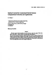
1.2 The Basic Idea Behind Model Predictive Control Model Predictive Control is, at the most basic level, a method of controlling dynamic systems using the tools of mathematical optimization. The common feature of all Model Predictive Control approaches is to solve on-line, at each sampling instant, a finite horizon optimal control problem based on a dynamic model of the plant, where the current state is the initial state. Only the first element of the computed sequence of predicted optimal control actions is then applied to the plant. At the next sampling instant, the prediction horizon is shifted, and the finite horizon optimal control problem is solved again for newly obtained state measurements. This idea is not new, already in Lee and Markus (1967) one can find the following statement: “One technique for obtaining a feedback controller synthesis from knowledge of open-loop controllers is to measure the current control process state and then compute very rapidly for the open-loop control function. The first portion of this function is then used during a short time interval, after which a new measurement of the process state is made and a new open-loop control function is computed for this new measurement. The procedure is then repeated.” The technique described by Lee and Markus (1967) is commonly referred to as “Receding Horizon Control” (RHC), and is today used more or less synonymously to the term Model Predictive Control.

Figure 1.1.: Receding Horizon Control (Bemporad and Morari (1999))

2

1. Introduction

Figure 1.1, which has been inspired by Bemporad and Morari (1999), illustrates the concept of Receding Horizon Control for a SISO system. At time t , the (open-loop) optimal control problem is solved for the initial state x(t) with a prediction horizon of length N . From the sequence of predicted optimal control ∗ ∗ ∗ inputs u (t) := u0 (t), . . . , uN −1 (t) , the first element u∗0 (t) is applied to the plant until the next sampling instant. At time t +1, the prediction horizon is shifted by one, new measurements of the state x(t +1) are obtained, and the optimal control problem is solved again for the new data. If the predictions were accurate and there was no uncertainty present, then of course the first N −1 elements of u∗ (t +1), would coincide with the last N −1 elements of u∗ (t). But since in reality there will always be some degree of uncertainty, u∗0 (t+1) will generally differ from u∗1 (t). Thus, repeatedly shifting the horizon and using new measurements of the state of the system provides some degree of robustness against modeling errors and perturbations. Receding Horizon Control therefore introduces feedback into the closed-loop system.

1.3 MPC – A Brief History and Current Developments The first practical applications of Model Predictive Control, at the time mainly in the process industry, date back already about 35 years (Garcia et al. (1989); Qin and Badgwell (2003); Camacho and Bordons (2004)). A variety of different versions of MPC emerged from the concepts of the first generation MPC methods like IDCOM (Richalet et al. (1978)) and DMC (Cutler and Ramaker (1980)). Lacking comprehensive theory, the use of MPC in industry until the late 1980’s was often times merely an ad-hoc solution, usually without formal guarantees on stability and feasibility of the solution. This began to change in the early 1990’s, when an increasing number of researchers in academia became interested in the theory of MPC. Since then, there has been a vast and ever increasing number of contributions to the field: In Morari (1994) it is reported that a simple database search for “predictive control” generated 128 references for the years 1991–1993 alone. Bemporad and Morari (1999) already reported 2.802 hits for the years 1991–1999. Today, “predictive control” generates more than 22.200 results for the years 1991–2010. The reason for the popularity of MPC in both industry and academia is simple: Model Predictive Control is one of the few (if not the only) control methodologies that can guarantee optimality (with respect to some performance measure) while ensuring the satisfaction of hard constraints on system states and inputs 1 . One of the main limitations of MPC has always been its substantial computational complexity in comparison to classical controller types. After all, a mathematical optimization problem has to be solved on-line at each sampling instant. Thus, the practical application of MPC in the past has been restricted to “slow” dynamical systems. This also explains the rather isolated success of MPC in the process industry, where time constants are usually relatively large, constraint satisfaction is essential, and the cost of expensive computer technology is of minor significance. During the last decade, the situation has however changed, and Model Predictive Control has become increasingly interesting for a wider range of applications. There are three important factors that contributed and still contribute to this development. The first one is the considerable progress in computer technology that allows the development of increasingly fast, cost-effective, miniaturized, and energy-efficient processors. The second important factor is the development of more powerful and more reliable optimization algorithms, that continuously widen the spectrum of possible applications of MPC methods. Finally, as a third factor, the theoretical advances in MPC itself must of course not be forgotten. After a consensus had been reached within the control community on what kind of “ingredients” were necessary to ensure stability and feasibility of MPC, a process which was more or less completed with the seminal survey paper Mayne et al. (2000), researchers have now turned themselves to the development of extensions to standard nominal Model Predictive Control. 1

Clearly, simply saturating the control action of unconstrained optimal controllers (i.e. LQR) is NOT an optimal control technique and may exhibit arbitrarily poor performance or even result in loss of stability.

1.3. MPC – A Brief History and Current Developments

3

In order to enable the application of Model Predictive Control to commonly encountered practical control problems, one of the main requirements is to be able to design controllers that are robust with respect to uncertainties. It is well known that nominal Model Predictive Controllers inherently provide some degree of robustness (de Nicolao et al. (1996); Santos and Biegler (1999)), yet this robustness is very hard to quantify and may even, except for linear systems subject to convex constraints, be arbitrarily small, as was pointed out in Teel (2004); Grimm et al. (2004). Because of the use of on-line optimization, Bemporad and Morari (1999) consider robustness analysis of MPC control loops generally far more difficult than their synthesis. This insight, together with the motivation coming from the success of Linear Robust Control theory (Green and Limebeer (1994); Zhou et al. (1996)), led to considerable research activity in “Robust MPC” (Bemporad and Morari (1999); Chisci et al. (2001); Cuzzola et al. (2002); Kothare et al. (1995); Mayne et al. (2005); Scokaert and Mayne (1998)). Robust MPC is, as Linear Robust Control is, a constructive technique that takes uncertainties (either in the model, or caused by exogenous disturbances) directly into account already during the design process of the controller. This field has recently seen a number of enticing contributions, and will be the main theme of this thesis in the chapters 3, 4 and 5. Another very interesting line of work in the field of linear MPC proposes to use parametric programming to precompute the solution of the optimal control problem (which is traditionally solved on-line for a measured initial state) for all initial states off-line, and to store the resulting piecewise-affine control law in a lookup table (Bemporad et al. (2002); Alessio and Bemporad (2009)). This method, commonly referred to as “Explicit MPC”, seems a promising alternative to conventional on-line optimization, at least for applications to fast systems of lower complexity (in terms of state dimension and number of constraints). As one recent example, Mariéthoz et al. (2009) report FPGA implementations of Explicit MPC that achieve sampling frequencies up to 2.5Mhz. The basic ideas of Explicit MPC will be presented in section 2.4. Moreover, Explicit Robust Model Predictive Controllers will also be implemented the context of Tube-Based Robust MPC and Interpolated Tube MPC in chapter 4 and 5, respectively. Other contributions include extensions of MPC to the output-feedback case, i.e. when only incomplete information about the system state is available, and to tracking problems (Mayne et al. (2000)), both of which will be addressed in this thesis. Current research on Model Predictive Control includes the development of suboptimal linear MPC algorithms (Zeilinger et al. (2008); Canale et al. (2009)) and the nonlinear Robust MPC (Lazar et al. (2008); Limon et al. (2009)). Due to the vast amount of available literature this thesis can not aim at giving an exhaustive overview over the developments and trends in the field of Model Predictive Control. The following chapters are therefore restricted to (Robust) Model Predictive Control for discrete-time constrained linear systems.

4

1. Introduction

2 Model Predictive Control for Constrained Linear Systems The purpose of the following chapter is to give a brief introduction to nominal Model Predictive Control of constrained discrete-time linear systems. The varieties of MPC are of course far greater than this limited view can provide, they include the design of controllers for nonlinear as well as for time-varying systems in both discrete and continuous time. At least the discrete-time formulation is however not really a restriction: Since the employed Receding Horizon Control strategy inherently introduces a discretization of time, it is only plausible to formulate the MPC problem in discrete time, and most researchers interested in implementable algorithms do so. The theory of nonlinear MPC1 is, although important progress has been made (Findeisen et al. (2007)), not yet as well developed as the one of linear MPC. Nonlinear MPC naturally involves more complex optimization problems than linear MPC does, a fact that immediately exacerbates the problem of developing sufficiently fast optimization algorithms for on-line implementation. So far there is also no method comparable to Explicit MPC for linear models (see section 2.4) in sight, only suboptimal approximative techniques based on linear multiparametric programming have been developed. Because of the named issues, nonlinear MPC will not be addressed any further in this thesis. The use of MPC for unconstrained linear systems is more than questionable, since LQR/LQG control is considered to solve this problem well (Bitmead et al. (1990)). In fact, is is easy to show that if the LQR infinite horizon cost is used as a terminal cost in the unconstrained MPC formulation, the LQR controller itself is recovered for any prediction horizon. Clearly, implementing this kind of controller would be an absurd thing to do. Over time, numerous different approaches to the question of how to ensure stability of the closed-loop system when using a Model Predictive Controller have been pursued in the literature, all of which have some important features in common. The following review will only encompass those ideas that in the process of a continuous refinement have been condensed out of these approaches and have become widely accepted in the Model Predictive Control community. For details, the reader is referred to the excellent survey paper Mayne et al. (2000) and the recent book Rawlings and Mayne (2009), on which much of the content and notation of this introductory section is based. In order to allow for an overall coherent exposition, this basic notation will also be adopted (and, if necessary, extended) throughout the following chapters of this thesis. As its name suggests, Model Predictive Control is based on an underlying model of the process to be controlled. In the context of MPC for constrained linear systems one usually considers a discrete-time linear system of the form

x(t + 1) = Ax(t) + Bu(t) y(t) = C x(t),

(2.1)

where x(t) ∈ Rn , u(t) ∈ Rm and y(t) ∈ R p are the system state, the applied control action, and the system output at time t , respectively. The matrices A ∈ Rn×n , B ∈ Rn×m , and C ∈ R p×n are the system matrix, the input matrix and the output matrix, respectively. 1

nonlinear MPC refers to MPC of nonlinear models, as MPC is, even for linear systems, inherently nonlinear

5

System (2.1) is subject to the following constraints on state and input:

x(t) ∈ X,

u(t) ∈ U,

(2.2)

where the control constraint set U ⊂ Rm is convex and compact (closed and bounded), and the state constraint set X ⊂ Rn is convex and closed. Both U and X are assumed to contain the origin in their interior, i.e. 0 ∈ int(U) and 0 ∈ int(X).

2.1 The Regulation Problem For now, the attention will be restricted to the regulation problem only. In the regulation problem, the objective is to optimally (with respect to some performance measure) steer the state x(t) of system (2.1) to the origin while satisfying the constraints (2.2) at all times. In order for this to be an achievable goal, the following (reasonable) assumption is necessary and will be adopted throughout this thesis: Assumption 2.1: The pair (A, B) is controllable.

2.1.1 The Model Predictive Controller As with all Model Predictive Controllers, a Receding Horizon Control strategy as described in section 1.2 is employed to control the system (2.1). Hence, at each time step, a finite horizon optimal control problem needs to be solved. The cost function VN (·) of this optimal control problem is defined by

VN (x(t), u(t)) :=

t+N X−1

l(x i , ui ) + Vf (x t+N )

(2.3)

i=t

where N is the prediction horizon, u(t) := u t , u t+1 , . . . , u t+N −1 denotes the sequence of predicted control inputs and x(t) := x t , x t+1 , . . . , x t+N denotes the predicted state trajectory whose elements satisfy x i+1 = Ax i +Bui . For clarity it makes sense to distinguish between the notations x(t) and x t+i as follows: The argument in parentheses denotes actual values, whereas the subscript denotes predicted values. Thus, x(t) denotes the actual state of the system at time t , whereas x t+i denotes the predicted state of the system at time t + i , given the information about the system at time t . Because the current state is measured and the first element of the predicted control sequence is really applied to the system, the actual values of the respective elements x t and u t of u(t) and x(t) are given by x t = x(t) and u t =u(t). The stage cost function l(·, ·) in (2.3) is a positive definite function of both state x and control input u, satisfying l(0, 0) = 02 , and is usually chosen as

l(x i , ui ) := ||x i ||Q2 + ||ui ||2R

(2.4)

where ||x||Q2 := x T Q x and ||u||2R := u T R u denote the squared weighted euclidean norms with the positive definite state weighting matrix Q 0 and control weighting matrix R 0, respectively. Similarly, the terminal cost function Vf (·) is also a positive definite function of the state and satisfies Vf (0) = 0. For reasons that will become clear in the following sections, the terminal cost is usually chosen of the form

Vf (x t+N ) := ||x t+N ||2P

(2.5)

2

in the following 0 will denote the scalar zero, whereas 0 will denote the zero matrix or the zero vector of appropriate dimension. Similarly, I will denote the identity matrix of appropriate dimension

6

2. Model Predictive Control for Constrained Linear Systems

with a terminal weighting matrix P 0. In addition to the externally specified constraints (2.2), a terminal constraint of the form

x t+N ∈ X f

(2.6)

is imposed on the predicted terminal state x t+N . Remark 2.1 (Polytopic norms in the cost function): It is not necessary to use a cost function based on quadratic norms in the formulation of the optimization problem. The use of polytopic norms is beneficial from a computational point of view as it yields a Linear Program (LP), for which very efficient and reliable solvers exist. However, this type of cost may result in an inferior closed-loop behavior compared to the use of a quadratic cost (Rao and Rawlings (2000)). Since the system and its constraints are assumed to be time-invariant, it is possible to simplify notation by rewriting the system dynamics (2.1) as

x + = Ax + Bu y = C x,

(2.7)

where x + denotes the successor state of x . The cost function VN (·) only depends on the value of the current state and not on the current time t , therefore one may write

VN (x, u) :=

N −1 X

l(x i , ui ) + Vf (x N ),

(2.8)

i=0

where u := u0 , u1 , . . . , uN −1 and x := {x 0 , x 1 , . . . , x N −1 }, with x 0 := x . This formulation is equivalent to (2.3). Let Φ(i; x, u) denote the solution of (2.7) at time i controlled by u when the initial state at time 0 is x (by convention, Φ(0; x, u) = x ). Furthermore, for a given state x , denote by UN (x) the set of admissible control sequences u, i.e. ¦ © UN (x) = u | ui ∈ U, Φ(i; x, u) ∈ X for i =0, 1, . . . , N −1, Φ(N ; x, u) ∈ X f . (2.9) Let XN denote the domain of the value function VN∗ (·), i.e. the set of initial states x for which the the set of admissible control sequences UN (x) is non-empty: XN = x | UN (x) 6= ; . (2.10) Usually, one refers to XN as the region of attraction of the Model Predictive Controller. At each time t , it is assumed that the current state x of the system is known. The sequence of optimal predicted control inputs u∗ (x) for a given state x is obtained by minimizing the cost function (2.8). Denote by PN (x) the following finite horizon constrained optimal control problem: VN∗ (x) = min VN (x, u) | u ∈ UN (x) (2.11) u u∗ (x) = arg min VN (x, u) | u ∈ UN (x) . (2.12) u

At each sampling instant, PN (x) is solved on-line, and the first element u∗0 (x) of the predicted optimal control sequence u∗ (x) is applied to the system. The repeated execution of measuring the state, computing the optimal control input and applying it to the plant can be regarded as an implicit time-invariant Model Predictive Control law κN (·) of the form

κN (x) := u∗0 (x).

(2.13)

The dynamics of the closed-loop system can then be expressed as

x + = Ax + BκN (x) y = C x. 2.1. The Regulation Problem

(2.14) 7

2.1.2 Stability of the Closed-Loop System In order to discuss the parameter choices that are necessary to guarantee stability and feasibility of the Model Predictive Controller, the notion of a positively invariant set is required. Invariant sets play an important role in Control Theory and are used extensively especially in Model Predictive Control (Raković (2009)). For a detailed treatment of the theory and application of set invariance in controls, the reader is pointed to the very good survey paper Blanchini (1999) and the recent book Blanchini and Miani (2008). Definition 2.1 (Positively invariant set, Blanchini (1999)): A set Ω is said to be positively invariant (PI) for the autonomous system x(t + 1) = f (x(t)) if, for all x(0) ∈ Ω, then the solution x(t) ∈ Ω for all t > 0. Corollary 2.1 (Positive invariance for closed-loop linear systems): Let κ(·) : Rn 7→ Rm be a state-feedback controller (not necessarily a linear one). A set Ω ⊆ Rn is positively invariant for the closed-loop system (2.14) if, for all x ∈ Ω, then Ax + Bκ(x) ∈ Ω. Stability of MPC is usually established using Lyapunov arguments, where the optimal cost VN∗ (·) is used as a Control Lyapunov Function (CLF). The additional assumptions on the terminal set X f and the terminal cost function Vf (·) that are necessary to ensure stability and feasibility of the closed-loop system (2.14) can be summarized as follows: Assumption 2.2 (Mayne et al. (2000)): 1. All states inside the terminal set X f satisfy the state constraints, X f is closed, and it contains the origin, i.e. 0 ∈ X f ⊂ X 2. The control constraints are satisfied inside the terminal set, i.e. κ f (x) ∈ U, ∀x ∈ X f , where κ f (·) : Rn 7→ Rm is a local state-feedback controller 3. The terminal set X f is positively invariant under κ f (·), i.e. Ax + Bκ f (x) ∈ X f , ∀x ∈ X f 4. The terminal cost function Vf (·) is a local Control-Lyapunov function (CLF), i.e. Vf (Ax + Bκ f (x)) ≤ Vf (x) − l(x, κ f (x)), ∀x ∈ X f Assumption 2.2 is straightforward: items 1 and 2 ensure feasibility of the origin, of all states within the terminal set X f , and of all control actions generated by the terminal feedback controller κ f (·) acting on any state within X f . Item 3 ensures persistent feasibility of the states and control inputs beyond the actual prediction horizon N while item 4 ensures stability by requiring that the terminal cost along the trajectory of the closed-loop system controlled by terminal controller κ f (·) is non-increasing. The following theorem states the main stability result for nominal MPC for constrained linear systems: Theorem 2.1 (MPC stability, Rawlings and Mayne (2009)): Suppose that the cost function is of the form (2.8) and that Assumption 2.2 holds. Then, if XN is bounded, the origin is exponentially stable with a region of attraction XN for the system x + = Ax +BκN (x). If XN is unbounded, the origin is exponentially stable with a region of attraction that is any sublevel set of VN∗ (·). Although the policy of this thesis is to generally refrain from stating proofs for results drawn from external references (and instead point the reader to the corresponding references), an exception will be made for the above theorem. The reason for doing this is that Theorem 2.1 is a fundamental basis for everything that will be presented in the later chapters of this thesis. Furthermore, the proof serves as a template for more or less all MPC stability proofs, and its basic idea can be found throughout the MPC literature and other proofs within this thesis. The proof of Theorem 2.1 is given in Appendix A.1. 8


2.1.3 Choosing the Terminal Set and Terminal Cost Function Theorem 2.1 merely requires the terminal cost function Vf (·) to be any local CLF for the system (2.7). Clearly, if Vf (·) was chosen as the infinite horizon cost function V∞∗ (·) (obtained by taking the limit N → ∞ in (2.8)), then, by the principle of optimality (Bertsekas (2007)), VN∗ (·) = V∞∗ (·). Regardless of the prediction horizon N , infinite horizon optimal control would be recovered. However, due to the presence of the constraints, V∞∗ (·) is unknown. A common move in MPC therefore is to choose Vf (·) as V˜∞ (·), the cost of the unconstrained infinite horizon optimal control problem:

V˜∞∗ (x) = min u

∞ X i=0

l(x i , ui ) = min u

∞ X

||x i ||Q2 + ||ui ||2R

(2.15)

i=0

The solution of (2.15) is the well known solution of the classic discrete-time LQR problem, i.e.

V˜∞∗ (x) = ||x|| P∞ = x T P∞ x,

(2.16)

with P∞ being the unique positive definite solution to the Discrete-Time Algebraic Riccati Equation (ARE) −1

P∞ = Q + AT (P∞ − P∞ B(R + B T P∞ B)

B T P∞ ) A.

(2.17)

The optimal linear feedback controller that minimizes (2.15) (often times referred to as “Kalman-Gain”) −1 is given as K∞ = −(R + B T P∞ B) B T P∞ A. If one chooses Vf (·) = V˜∞∗ (·) or, equivalently, P = P∞ in (2.5), Assumption 2.2 requires the terminal set X f to be positive invariant under κ f (x) = K∞ x , and that state and control constraints be satisfied, i.e. X f ⊂ X and κ f (x) ∈ U for all x ∈ X f . A set that satisfies the above is called a constraint admissible positively invariant set. Definition 2.2 (Constraint admissible positively invariant set, Kerrigan (2000)): Consider the autonomous system x + = (A+ BK)x subject to the constraints x ∈X and K x ∈U. A positively invariant set Ω for this system is constraint admissible if Ω ⊆ X and KΩ ⊆ U. The essential role of the terminal set X f is to permit the replacement of the actual infinite horizon cost V∞∗ (·) by the infinite horizon cost V˜∞∗ (·) of the unconstrained system (Mayne et al. (2000)). In order to obtain a region of attraction XN of the Model Predictive Controller as large as possible, X f is usually chosen as the maximal positively invariant set for the closed-loop system x + = (A + BK∞ )x . Definition 2.3 (Maximal positively invariant set, Kerrigan (2000)): A constraint admissible positively invariant set Ω for the autonomous system x + = (A + BK)x subject to the constraints x ∈ X and K x ∈ U is said to be the maximal positive invariant (MPI) set Ω∞ if 0 ∈ Ω∞ and Ω∞ contains every constraint admissible invariant set that contains the origin. Note that there is quite a variety of different definitions for invariant sets in the literature. All of these definitions differ slightly from each other, but basically describe the same concepts. One well-known definition is for example that of the maximal output admissible set (Gilbert and Tan (1991)), which is essentially the same as the definition of the maximal positively invariant set used in this thesis. For the previously assumed case that the state constraint set X contains an open region around the origin, Gilbert and Tan (1991); Kolmanovsky and Gilbert (1998) show that if A + BK∞ is Hurwitz3 (which can always be achieved if Assumption 2.1 holds true), the MPI set Ω∞ exists and contains a nonempty region around the origin. Clearly, if the terminal set X f is chosen as the MPI set Ω∞ it follows from Definition 2.3 that Vf (x) = V˜∞∗ (x) for all x ∈ X f . 3

a quadratic matrix is Hurwitz when all its eigenvalues lie strictly inside the unit disk

2.1. The Regulation Problem

9

The following Lemma states two interesting results about the optimality of the solution obtained from the constrained finite horizon optimal control problem PN (x). Lemma 2.1 (Optimality of the solution): Let Vf (·) = V˜∞ (·) in the cost function (2.8), and let Assumption 2.2 be satisfied. Then, 1. VN∗ (x) = V∞∗ (x) for all x ∈X f 2. VN∗ (x) = V∞∗ (x) for all x ∈ XN for which the terminal constraint x N ∈ X f is inactive in problem PN (x)

Proof. Both items 1 and 2 of Lemma 2.1follow directly from the principle of optimality (Bertsekas (2007)) and from the fact that Vf (x) = V˜∞∗ (x) for all x ∈ X f . Remark 2.2 (Synthesizing controllers that provide “real” optimality): Item 1 in Lemma 2.1 states that the unconstrained LQR controller is recovered for all initial states x ∈ X f . This is because for all states within the terminal set X f the unconstrained LQR controller is persistently feasible and hence optimal. Item 2 states the less obvious fact that in case the terminal constraint is inactive, the optimal cost VN∗ (x) of the finite horizon optimal control problem PN (x) is equal to the optimal cost V∞∗ (x) of the constrained infinite horizon optimal control problem. An interesting approach that somewhat reversely exploits this fact is taken by the authors of Sznaier and Damborg (1987); Scokaert and Rawlings (1998). They propose to employ a variable prediction horizon N in the following fashion: At each time step, problem PN (x) is solved without explicitly invoking the terminal constraint x N ∈ X f for increasing prediction horizons N , starting from some small initial horizon N0 . The prediction horizon is then increased until the predicted terminal state satisfies x N ∈ X f . A similar approach was proposed in the context of switched linear systems by Balandat et al. (2010).

2.1.4 Solving the Optimization Problem In order to implement a Model Predictive Controller in practice, the optimization problem PN (x) from page 7 must be solved on-line at each sampling instant4 . If stage and terminal cost in the cost function (2.8) are chosen as (2.4) and (2.5), respectively, the objective function VN (x, u) of PN (x) is quadratic. The state and control weighting matrices Q and R are given and the terminal weighting matrix P is easily obtained by solving the ARE (2.17) of the associated unconstrained LQR problem off-line using standard algorithms. So far there have been no assumptions made on the nature of the constraint sets X, U and X f . In case these sets are polytopic (i.e. they can be represented by the intersection of a finite set of closed halfspaces (Ziegler (1995))), then the optimization problem PN (x) becomes comparably easy to solve. Therefore, the common assumption made in the literature is the following: Assumption 2.3 (Nature of the constraint sets): The constraint sets X, U and X f in problem PN (x) are polytopic. Remark 2.3 (Implied polytopic shape): Note that it in Assumption 2.3 it would actually be sufficient to only assume that X and U are polytopic. This is because linearity of the system then implies that the maximal positively invariant set, which will usually be the choice for X f , is also polytopic (Gilbert and Tan (1991); Kolmanovsky and Gilbert (1998)). 4

10

There exist MPC algorithms that skip measurements and apply the computed optimal control input with some delay, hence allowing for more than one sampling interval for solving PN (x). This however significantly complicates analysis in the presence of uncertainty. Therefore, these and other variants of MPC are not considered here for simplicity


Under Assumption 2.3, the optimization problem PN (x) can be posed as

VN∗ (x) =

min

u0 ,...,uN −1 x 0 ,...,x N

s.t.

x NT P x N +

N −1 X

x iT Qx i + uiT Rui

i=0

x i+1 = Ax i + Bui

i = 0, . . . , N −1

x0 = x H x xi ≤ kx

i = 0, . . . , N −1

Hu ui ≤ ku

i = 0, . . . , N −1

(2.18)

H f xN ≤ kf , where X = {x | H x x ≤ k x }, U = {u | Hu u ≤ ku } and X f = {x | H f x ≤ k f } are the “H -representations” (Ziegler (1995)) of the respective polyhedral sets. Clearly, (2.18) is a Quadratic Programming problem (QP), which can be solved fast, efficiently and reliably using modern optimization algorithms (Boyd and Vandenberghe (2004); Nocedal and Wright (2006); Dostál (2009)). Obtaining the Terminal Set X f The only remaining question now concerns the computation of the terminal set X f . As outlined in Gilbert and Tan (1991); Blanchini (1999); Blanchini and Miani (2008), there exist efficient algorithms for the computation of (polytopic) maximal positively invariant sets for polytopic constraint sets. Hence, with the Kalman-gain K∞ obtained from the unconstrained LQR problem, the terminal set X f can easily be computed off-line as the maximal positively invariant set Ω∞ of the closed-loop system x + = (A + BK∞ )x . An algorithm for the computation of Ω∞ as well as some computational issues pertaining to it will be discussed in section 4.5.1 in the context of Tube-Based Robust MPC.

2.2 Robustness Issues and Output-Feedback Model Predictive Control An important question that arises in the assessment of any control strategy is how well the controller deals with uncertainty. In Model Predictive Control this question is: What happens if, due to the effects of uncertainty, the predicted evolution of the nominal system is different from its actual behavior? At best, the only thing that will happen when the nominal controller is used for the uncertain system is a degradation in performance. But if the uncertainty is “large”, or if the closed-loop system has small robustness margins, the controlled uncertain system may also become unstable. The Robust Control issue is generally much harder to come by for constrained systems, as the control objective is to not only ensure robust stability but also robust constraint satisfaction. The causes of uncertainty are manifold: there may be modeling errors, the state of the system may not be exactly known, or exogenous disturbances may affect the system. Evidently, all of the above applies, at least to some degree, to virtually any practical application. Hence, it is clear that controllers need to be robust with respect to these uncertainties. Chapter 3 therefore introduces the Robust MPC framework, whose objective is to synthesize robust controllers based on some underlying model of the uncertainty. Output-Feedback Model Predictive Control One particular kind of uncertainty which is prevalent in more or less any real-world situation are measurement errors. The previous sections dealt with the design of Model Predictive Controllers based on the exact knowledge of the current state x of the system. In applications however, exact measurements of all system states are generally not available. Thus, it is necessary to develop extensions of the classic “state-feedback MPC” to “output-feedback MPC”, which only use the available (possibly inaccurate) measurements of the system’s output y .

2.2. Robustness Issues and Output-Feedback Model Predictive Control

11

It is standard practice in control engineering to combine a state-feedback controller with an observer that estimates the system state x from the available measurements y (Skogestad and Postlethwaite (2005)). If the observer is chosen as a Kalman-Filter (Kalman (1960)) this approach is usually referred to as “LQG-Control”. In virtue of the separation principle (Luenberger (1971)), closed-loop stability can then be ensured for the composite (linear) system. However, due to the nonlinear control law, the separation principle in general does not hold for systems controlled by Model Predictive Controllers (Teel and Praly (1995)). As a result things become more involved and additional caution is needed in the design of output-feedback MPC. Albeit numerous reasons for why it is actually not a great idea, nominal Model Predictive Controllers in loop with separately designed observers to date are still widely used in industry (Rawlings and Mayne (2009)). A variety of different ideas for a more theoretical approach to output-feedback MPC have been proposed in the literature (Bemporad and Garulli (2000); Löfberg (2002); Chisci and Zappa (2002); Findeisen et al. (2003)). A brief overview over some important contributions is given in section 3.6.1 in the context of Robust MPC. Moreover, the recently proposed and very elegant method of “output-feedback Tube-Based Robust Model Predictive Control” will be presented in more detail in chapter 4.

2.3 Reference Tracking So far the exposition has been concerned solely with the MPC regulation problem, the goal of which is to steer the system state to the origin. But what application engineers are really interested in is to optimally track a given output reference trajectory y r e f (t), while ensuring that state and control constraints are satisfied at all times. Obtaining general theoretical results on stability, feasibility, and robustness for constrained tracking of arbitrary, time-varying references is however extremely hard. Instead, the tracking problem is often confined to the problem of optimally tracking arbitrary, but constant reference signals y r e f (t) = ys . This is commonly referred to as “set point tracking”. The following sections will give a short introduction on how constrained set point tracking controllers can be realized using Model Predictive Control methods.

2.3.1 Nominal Set Point Tracking Model Predictive Control Set Point Characterization For the purpose of this section, assume that there is no uncertainty present. In this case, for the output y(t) of system (2.1) to be able to track a constant reference signal ys (set point) without exhibiting any offset, there must exist a feasible steady state5 (x s , us ) ∈ X × U satisfying

x s = Ax s + Bus

(2.19)

ys = C x s .

(2.20)

Hence, for any set point ys , there must exist a steady state input us such that

C(I − A)−1 B us = ys .

(2.21)

In order to hold for arbitrary set points ys ∈ R p , the mapping in (2.21) needs to be surjective, i.e. the matrix C(I − A)−1 B ∈ R p×m must have full row rank. The following Lemma states an equivalent condition: 5

12

with some abuse of notation the pair (x s , us ) of actual steady-state x s and associated constant control input us will in the following simply be referred to as “the steady state”


Lemma 2.2 (Pannocchia and Rawlings (2003)): Consider the linear discrete-time system (2.1). If and only if I − A −B rank = n + p, C 0

(2.22)

then there exists an offset-free steady state (x s , us ) for any constant set point ys . Remark 2.4 (Pannocchia and Rawlings (2003); Pannocchia and Kerrigan (2005)): Note that condition (2.22) in Lemma 2.2 implies that the number of controlled variables cannot exceed either the number of control inputs or the number of states, i.e. p ≤ min{m, n}. If (2.22) holds true then the steady state (x s , us ) is not necessarily unique for a given set point ys . If this is the case, a common approach (Muske and Rawlings (1993); Scokaert and Rawlings (1999)) is to determine artificially a unique steady state (x s∗ , u∗s ) by solving the following quadratic optimization problem:

(x s∗ , u∗s ) = arg min (us − ud ) T Rs (us − ud ) x s ,us

x s = Ax s + Bus

s.t.

ys = C x s

(2.23)

xs ∈ X us ∈ U, where ud is a desired steady state input and Rs 0 is a positive definite weighting matrix penalizing the deviation of us from ud . The equality constraints in (2.23) hereby ensure that the obtained pair (x s∗ , u∗s ) is indeed a steady state for the system (2.1). Obviously, if ud is an admissible steady state input, then u∗s = ud . If, on the other hand, the system does not provide enough degrees of freedom to track the desired reference ys without offset, one can determine a feasible steady state (x s∗ , u∗s ) such that the output tracking error is minimized in the least-squares sense (Muske and Rawlings (1993); Muske (1997)) by solving the following quadratic program:

(x s∗ , u∗s ) = arg min ( ys − C x s ) T Q s ( ys − C x s ) x s ,us

x s = Ax s + Bus

s.t.

(2.24)

x s ∈ X, us ∈ U, where Q s 0 is a positive definite weighting matrix penalizing the output tracking error. The actual output that is achieved at steady state then is ˜ys = C x s∗ . For the purpose of the remainder of this section it will be assumed that the condition in Lemma 2.2 is satisfied, i.e. that for any target set point ys there exists feasible offset-free steady state (x s , us ). Nominal Model Predictive Control for Tracking Given an offset-free steady state pair (x s ( ys ), us ( ys )) for the desired set point ys , a Tracking Model Predictive Controller (Rawlings and Mayne (2009)) is realized by solving on-line the modified optimal control problem PN (x, ys )

VN∗ (x, ys ) = min VN (x, ys , u) | u ∈ UN (x, ys ) u u∗ (x, ys ) = arg min VN (x, ys , u) | u ∈ UN (x, ys ) , u

2.3. Reference Tracking

(2.25) (2.26) 13

in which the cost function VN (·) and the set of admissible control sequences UN , which now both depend on the value of the target set point ys , are defined by

VN (x, ys , u) :=

N −1 X

l(x i − x s ( ys ) , ui − us ( ys )) + Vf (x N − x s ( ys ))

(2.27)

i=0

¦ © UN (x, ys ) = u | ui ∈ U, Φ(i; x, u) ∈ X for i =0, 1, . . . , N −1, Φ(N ; x, u) ∈ X f ( ys ) .

(2.28)

Terminal cost function Vf (·) and stage cost function l(·, ·) are again chosen as (2.5) and (2.4), the respective cost functions used in the regulation problem. The reference-dependent terminal set X f ( ys ) can, since the system is linear, be chosen as a shifted version of the terminal set X f from the regulation problem (which is centered at the origin), i.e.6

X f ( ys ) = x s ( ys ) ⊕ X f ⊂ X,

(2.29)

where the steady state x s ( ys ) must satisfy the additional constraint that all states within the shifted terminal set X f ( ys ) be contained in X. This additional requirement limits the set points that can be tracked to the set ¦ © Ys := ys | x s ( ys ) ⊕ X f ∈ X, us ( ys ) ∈ U . (2.30) For a given admissible set point ys ∈ Ys the region of attraction XN of the tracking controller is

XN ( ys ) := x | UN (x, ys ) 6= ; .

(2.31)

Remark 2.5 (Choice of the terminal set): Note that it is not possible to simply use a terminal set of the form {x s ( ys )} ⊕ X f ∩ X, as this set, in general, is not positively invariant and therefore does not ensure persistent feasibility of the closed-loop system beyond the prediction horizon. One possible way to enlarge the set of trackable set points Ys is to choose a terminal set of the form x s ( ys ) ⊕ αX f with α ∈ [0, 1], which is positively invariant (because of linearity). However, this choice at the same time yields a controller with a smaller region of attraction XN . Alternatively, an appropriate positively invariant terminal set could be recomputed on-line for each new set point ys . The on-line computation of positively invariant sets is however computationally prohibitive in general. Employing the Receding Horizon Control approach and applying only the first element u∗0 (x, ys ) of the predicted sequence u∗ (x, ys ) of optimal control inputs to the system, the implicit Model Predictive Control law is given by

κN (x, ys ) := u∗0 (x, ys ).

(2.32)

Stability of the steady state (and hence of the set point ys ) can be established as follows: Corollary 2.2 (Stability of nominal Tracking MPC, Rawlings and Mayne (2009)): Suppose that the rank condition (2.22) holds, that ys ∈Ys is an admissible constant reference set point, and that (x s ( ys ), us ( ys )) is an associated steady state of the system satisfying both state and control constraints. Furthermore, suppose that the cost function is of the form (2.27) and that Assumption 2.2 holds with the terminal set X f ( ys ) as in (2.29). Then, stable with the steady state x s ( ys ) is exponentially + a region of attraction XN ( ys ) = x | UN (x, ys ) 6= ; for the closed-loop system x = Ax + BκN (x, ys ). 6

14

in (2.29) the so-called Minkowski set addition, denoted by ⊕, is used. Its formal definition is postponed to Definition 4.3 to allow for a more coherent presentation of chapter 4. Here it can simply be seen as shifting the set X f by x s ( ys )


As indicated in Remark 2.5, Tracking MPC is generally more involved than just shifting the system to the desired steady state. In particular, for this approach to be feasible it is necessary that (2.29) is satisfied. This requirement, however, may lead to a potentially small region of admissible steady states. For the regulation problem, one generally wants to use a terminal set X f as large as possible, such that the region of attraction XN of the controller is also large. If the size of X f is primarily limited by the state constraints X (meaning that the set U of feasible control actions is comparatively large), then (2.29) will be satisfied only for steady states x s close to to origin. Conversely, in order to enlarge the region of admissible steady states it is necessary to use a smaller terminal set X f . Hence, the method of shifting the original system to a desired steady state to achieve tracking is inherently a tradeoff. An Improved Approach to Tracking Model Predictive Control An elegant method for Tracking Model Predictive Control is developed in Limon et al. (2005, 2008a); Ferramosca et al. (2009a). The proposed controller features an additional artificial steady state to which the system is driven. An additional offset cost penalizing the deviation of the artificial steady state from the steady state corresponding to the output reference is introduced in the cost function. Since the constraints do not depend on the desired output reference, the controller ensures feasibility for all reference values and drives the system to the closest admissible steady state. The details of this approach will be discussed in the context of Tube-Based Robust MPC in chapter 4 of this thesis. A further extension developed in Ferramosca et al. (2009b, 2010) addresses the problems of tracking target sets, i.e. when the desired output reference is required to lie in a specific set in the output space, where the exact values of the outputs are not important.

2.3.2 Offset Problems in the Presence of Uncertainty In the previous sections, it was assumed that a perfect model of the system was available and that there were no external disturbances present. In this nominal case, if there exists a feasible steady state for the given output set point ys , offset-free tracking is achieved, i.e. lim t→∞ y(t) = ys . In real-world applications, however, perfect models do not exist and the system will always be subject to some exogenous disturbance. It is well known that if there is a non-vanishing disturbance (with zero mean) present, standard Model Predictive Control methods as discussed in the previous sections generally exhibits offset, i.e. there is a mismatch between measured and predicted outputs. This is true for both tracking controllers and regulators (clearly, ys,r e g = x s,r e g = us,r e g = 0). The prevailing approach in the literature to overcome this deficiency is to augment the system state with fictitious integrating disturbances (Maeder et al. (2009); Muske and Badgwell (2002); Pannocchia and Kerrigan (2005); Pannocchia (2004); Pannocchia and Rawlings (2003)). By doing so it is possible, under proper conditions, to achieve offset-free MPC given that the external disturbance is asymptotically constant. This idea will be revisited in more detail in section 3.6.3. In the context of Tube-Based Robust MPC, section 4.4.3 furthermore presents a method that enables offset-free control without augmenting the system state. This is achieved by determining the offset value from the measured output and a state estimate, and by scaling the reference input appropriately such that this offset is cancelled.

2.3.3 Reference Governors As another way of addressing the constrained tracking control problem, so-called “reference governors” (also: “command governors”) have been proposed (Bemporad and Mosca (1994b,a, 1995); Gilbert et al. (1995); Bemporad et al. (1997)). The basic concept of reference governors is to separate the issue of constraint satisfaction from the issue of designing a stable closed-loop system. A reference governor is an auxiliary nonlinear device that operates between the external reference command and the input 2.3. Reference Tracking

15

Figure 2.1.: Reference governor block diagram (Gilbert and Kolmanovsky (2002))

to the primal compensated control system, as depicted in Figure 2.1. The primal plant compensation, which may be performed using a wide range of different controller synthesis methods, yields a stable closed-loop system that performs satisfactorily in the absence of constraints. Whenever it is necessary, the reference governor modifies the reference input y r e f (t), generating a virtual reference input y r∗e f (t) so as to avoid constraint violation of the pre-compensated system. The necessary modification of y r e f (t) can be performed in different ways: While Bemporad and Mosca (1994a); Bemporad et al. (1997); Casavola and Mosca (1996); Chisci and Zappa (2003) and related concepts employ forms of Model Predictive Control, the approach advocated by Gilbert et al. (1994, 1995) uses a nonlinear low-pass filter. The MPC-based approach generates the virtual reference input y r∗e f (t) by solving on-line a mathematical optimization problem. The nonlinear filter, on the other hand, attenuates, if necessary, the external reference input y r e f (t) appropriately. In addition to the nominal case, robust reference governors have been proposed for uncertain systems in Casavola and Mosca (1996); Gilbert and Kolmanovsky (1999a); Casavola et al. (2000b). These approaches take uncertainties in the model and external disturbances directly into account. Moreover, the ideas behind reference governors have also been used for the purpose of controlling nonlinear systems (Bemporad (1998b); Angeli and Mosca (1999); Gilbert and Kolmanovsky (1999b, 2002)). Reference governors are an interesting approach to guaranteeing constraint satisfaction, in particular as they leave the basic stability properties of the pre-compensated system untouched. This allows for a large flexibility in the design of controllers for the pre-stabilization of the plant. However, the resulting overall controller is clearly not “optimal” in the sense a Model Predictive Controller would be. Among other drawbacks, this usually results in smaller regions of attraction (Casavola et al. (2000a)). Nevertheless, reference governors are a useful tool in constrained control.

2.4 Explicit MPC Section 2.1.4 argues that modern optimization algorithms are able to solve the quadratic optimization problem that arises in linear MPC fast and efficiently. However, the computational effort may still exceed the available computing resources, especially when the objective is to control fast7 processes with limited hardware resources. A very interesting approach to overcome this problem was proposed in the seminal paper by Bemporad et al. (2002), where the authors advocated the explicit solution of the optimization problem (2.18). The proposed approach is based on multiparametric programming, for which the current state x of the system is regarded as a parameter vector in the optimization problem. This way, the on-line computation effort can be reduced to a simple function evaluation (of a piece-wise affine optimizer function defined over polytopic regions in the state space). The following sections discuss only the basic ideas and properties of Explicit MPC, for further reading consult Bemporad et al. (2002); Tøndel et al. (2003b); Alessio and Bemporad (2009); Borrelli et al. (2010). Explicit controllers will also be implemented in the context of Tube-Based Robust MPC and Interpolated Tube MPC in chapter 4 and 5. 7

16

the definition of “fast” is of course constantly changing with the rapid progress in computer technology


2.4.1 Obtaining an Explicit Control Law In section 2.1.4 it has been shown how the on-line optimization problem PN (x) of a nominal Model Predictive Controller is readily formulated as the quadratic programming problem (2.18). By substituting Pi−1 x i = Ai x + j=0 A j Bui−1− j and performing a (linear) change of variables, the optimization problem (2.18) can be rewritten in the new variable z as

VN∗ (x) = min z T Hz z

s.t.

(2.33)

Gz ≤ W + S x,

where H 0, G , W and S are suitably defined matrices depending on the system dynamics and the constraints (Bemporad et al. (2002)). Note that in (2.33) the parameter vector x appears only on the right hand side of the constraints. This renders the problem a multiparametric Quadratic Program (mpQP), for which an explicit solution can be obtained. The properties of this solution are summarized in the following important theorem: Theorem 2.2 (Properties of the explicit solution, Bemporad et al. (2002); Alessio and Bemporad (2009)): Consider a multiparametric Quadratic Program of the form (2.33) with H 0. The set XN of parameters x for which the problem is feasible is a polyhedral set, the value function VN∗ : XN 7→ R is continuous, convex, and piecewise quadratic (PWQ), and the optimizer function z ∗ : XN 7→ RN ×m is piecewise affine (PWA) and continuous. Because of the linearity of the change of variables, the properties of the optimizer z ∗ from Theorem 2.2 are inherited by the optimal control sequence u∗ (x) and hence also hold for the Model Predictive Control law κN (x) := u∗0 (x). In contrast to the on-line solution, this control law can be stated explicitly as

 κN (x) =



F1 x + g1 .. .

if .. .

H1 x ≤ k1 .. .



FNr eg x + g Nr eg

if

H Nr eg x ≤ kNr eg

(2.34)

where κN ,l (x) = Fl x + g l is the affine control law defined on the l th polyhedral region Pl := x | H l x ≤ kl of the solution. The domain XN of the value function VN∗ (·) is partitioned into Nr eg different polyhedral S Nr e g regions, i.e. l=1 Pl = XN . In case the constraint set X is unbounded, it is futhermore necessary to explicitly specify a so-called exploration region X x pl , since in this case the set XN may also be unbounded. Specifying an exploration region (that should contain the desired operation region of the controller) is however recommendable in any case, since otherwise the number of regions Nr eg over which the controller is defined can grow very large (see section 2.4.2). A number of different algorithms for the computation of the polyhedral regions Pl and the associated affine state-feedback control laws κN ,l (·) have been developed (Alessio and Bemporad (2009); Bemporad et al. (2002, 2001); Spjøtvold et al. (2006); Tøndel et al. (2003b)). A common feature of these algorithms is that they are based on the first-order Karush-Kuhn-Tucker (KKT) optimality conditions (Boyd and Vandenberghe (2004)) for (2.33), from which they identify “sets of active constraints” that characterize so-called “critical regions” in the x -space. The region of attraction XN is then successively explored by obtaining the critical regions for all possible sets of active constraints. The algorithms differ mainly in the exploration strategy they use for covering the region of attraction with critical regions. The computation of the polyhedral partition and the piece-wise affine control law can be performed off-line, which reduces the on-line computation to a simple evaluation of (2.34). This allows the implementation of MPC controllers also for fast dynamic systems with high sampling frequencies (Alessio and Bemporad (2009)). 2.4. Explicit MPC

17

Remark 2.6 (Other benefits of Explicit MPC): An additional, more subtle benefit of Explicit MPC is that guarantees on the solution (such as an upper bound on the computation time, etc.) are comparably easy to derive, since all computations involving mathematical optimization algorithms are performed off-line. If instead on-line optimization is carried out “in the loop”, it is generally very hard to obtain formal guarantees that are not excessively conservative, since everything depends on the (potentially very complex, often also closed-source8 ) optimization algorithm. This benefit of Explicit MPC is especially useful in safety-critical applications such as aerospace engineering, which are subject to rigorous software certification processes. Naturally, the approaches and algorithms of Explicit MPC can be applied to any optimization problem that can be brought in the form (2.33). This includes other types of Model Predictive Controllers (e.g. the tracking controller from section 2.3), but more generally any optimization problem that depends affinely on a parameter, and that needs to be solved repeatedly at high speeds.

2.4.2 Issues with Explicit MPC Complexity of the Solution Although Explicit MPC seems a compelling alternative to on-line optimization at the first glance, there are also some drawbacks associated with it. A major problem is the growth of the number of regions Nr e g into which the domain XN is partitioned (Alessio and Bemporad (2009); Borrelli et al. (2010)). Although Nr eg grows only moderately with the state dimension (there is no “curse of dimensionality”), it depends, in the worst case, exponentially on the number of constraints in (2.33) (Bemporad et al. (2002)). The number of constraints again primarily depends on NX , NU , and NX f , the numbers of inequalities9 defining the polytopic sets X, U, and X f , respectively. From that it is obvious that the constraint sets should be chosen as simple as possible. Furthermore, since the number of constraints increases linearly with the prediction horizon N , exact Explicit MPC is limited to comparably short prediction horizons. Different ideas have been presented in the literature that aim at reducing the complexity of Explicit Model Predictive Controllers. Geyer et al. (2008) propose to merge those regions P for which the affine gain F x + g is the same, so that the exact solution of the problem is expressed with a minimal number of partitions. Other approaches introduce sub-optimality in order to reduce the complexity of the explicit solution (Grieder and Morari (2003); Bemporad and Filippi (2003); Rossiter and Grieder (2004); Rossiter et al. (2005); Pannocchia et al. (2007); Christophersen et al. (2007)). Yet another way is the use of semi-explicit methods as in Zeilinger et al. (2008), which pre-process off-line as much as possible of the MPC optimization problem without characterizing all possible outcomes, but rather leave some optimization operations for on-line computation. These topics as well as some further ideas are well discussed in the survey paper Alessio and Bemporad (2009). Controller Implementation The on-line evaluation of the piecewise state-feedback control law (2.34) requires the determination of the polyhedron in which the measured state x of the system lies. This information is crucial in order to decide which “piece” of the piece-wise affine control law to apply to the plant. This procedure has been referred to as the “point location problem” in the literature. The easiest and most straightforward way to implement an algorithm would be to store the polyhedral regions Pl and perform an on-line search through them until the region Pl ∗ which contains the current state x of the system is identified. The optimal control action is then simply obtained as u∗ = Fl ∗ x + g l ∗ . However, this approach is, in general, not very efficient in terms of evaluation time. Since the evaluation time is crucial for fast-sampling systems, researchers have developed alternate methods, which are more efficient especially in case the 8 9

18

optimization software is a competitive business, companies will usually try everything to keep their code secret NX , NU , and NX f appear as the number of rows of H x , Hu , and H f in (2.18), respectively


solution is characterized by a large number of regions Nr eg . These advanced approaches are, for example, based on the the use of binary search trees (Tøndel et al. (2003a)), PWA descriptor functions (Borrelli et al. (2001a); Baotic et al. (2008)), reachability analysis (Spjotvold et al. (2006)) or minimal volume bounding boxes (Christophersen (2007)). Research on the point location problem is ongoing, and efficient methods to evaluate the explicit control law (2.34) will be a key prerequisite for the successful application of Explicit MPC in the future. Other Aspects One of the general shortcomings of Explicit MPC is that its underlying approach is hard to generalize to nonlinear MPC. Although general nonlinear optimization algorithms are undoubtedly considerably harder to implement in real-time than, for example, Quadratic Programming, the basic MPC ideas also apply to nonlinear problems (with appropriate modifications to the cost function and the terminal set). Exact multiparametric programming, however, is generally restricted to optimization problems with linear (mpLP) or quadratic (mpQP) cost functions subject to linear constraints. Therefore, approximative explicit solution to nonlinear MPC problems have been proposed (Johansen (2002, 2004); Grancharova and Johansen (2006)). Another drawback of Explicit MPC is that it is not possible to change parameters of the optimization problem (i.e. weighting matrices and constraints) on-line. If any parameter (except x of course, which is regarded as the parameter vector in the multiparametric program) in (2.33) needs to be adjusted, the explicit solution needs to be recomputed. This is not the case when the optimization problem is solved on-line10 . On-line optimization based controllers therefore provide more flexibility by the possibility of a quicker re-parametrization in applications.

2.4.3 Explicit MPC in Practice When Should Explicit MPC be Used? It is very hard to make a general statement about when and for what kind of problems the use of Explicit MPC is beneficial, since the complexity of the solution depends not only on the number of variables and constraints in the optimization problem but also on the internal structure of the very problem itself. This will become clear in the case studies of chapter 4, where different Explicit Tube-Based Robust Model Predictive Controllers are implemented and compared to controllers based on on-line optimization. In addition, research on advanced, on-line optimization based MPC approaches that use specially tailored solvers that exploit the structure of the optimization problem is ongoing and reported results, for example those in Ferreau et al. (2008); Milman and Davison (2008); Wang and Boyd (2008); Biegler and Zavala (2009); Richter et al. (2009, 2010), are promising. Those specialized solvers are fast enough to compete with Explicit MPC, in particular for problems of higher complexity. Finally, the semi-explicit variants of MPC mentioned in the previous section seem a suitable way of combining the advantages of both on-line and off-line implementations. Explicit MPC to date can not yet be considered a mature technology. Further research effort is necessary to yield a practically applicable framework that is suitable for a noteworthy number of real-world applications. Nevertheless, several successful applications of Explicit MPC have already been reported in the literature by various researchers. Successful Applications of Explicit MPC The potential speed of Explicit MPC has been impressively demonstrated in a number of applications, most of which were in automotive and power systems control. Alessio and Bemporad (2009) characterize the applications most suitable for Explicit MPC as fast-sampling problems (with a sampling time in the range of 1-50ms) of relatively small size (involving 1-2 manipulated inputs and 5-10 parameters). In the context of automotive control, Borrelli et al. (2001b, 2006) report the successful application of Explicit MPC (for hybrid systems) to traction control. Recently, there have also been increasing research efforts to 10

this does not mean that on-line optimization based MPC has “hot-plug” capabilities, since simply changing parameters of a running controller induces other problems that have to be accounted for, i.e. stability and/or feasibility issues

2.4. Explicit MPC

19

implement Explicit MPC in hardware, in order to make it suitable for applications with very high sampling frequencies that appear, for example, in mechatronics, the control of MEMS, automotive control, or power electronics. In this context, Johansen et al. (2007) showed that Explicit MPC implementations on an application specified integrated circuit (ASIC), which use about 20,000 gates, allow sampling frequencies in the Mhz range. The authors also identified that the main problem of this kind of implementation is that the memory requirements increase rapidly with the problem dimensions. In a more recent article, Mariéthoz et al. (2009) report an FPGA implementation of Explicit MPC for a buck DC-DC converter that achieves sampling frequencies of up to 2.5Mhz. Software for Explicit MPC Algorithms for multiparametric programming and other tasks pertaining to the design of Explicit Model Predictive Controllers are implemented in the free Multiparametric Toolbox (MPT) for MATLAB (Kvasnica et al. (2004)). The Hybrid Toolbox (Bemporad (2004)), also free and developed for MATLAB, provides similar and some extended features. Note that the commercial Model Predictive Control Toolbox for MATLAB (Bemporad et al. (2010)) to date does not support the synthesis of Explicit Model Predictive Controllers (as of version 3.2).

20


3 Robust Model Predictive Control Although nominal Model Predictive Control as discussed in the previous chapter provides strong theoretical results about nominal stability and feasibility, it does not consider the question of what happens when the predicted system evolution differs from the actual system behavior. It has become a widely accepted consensus that for practical applications, Model Predictive Controllers need not only guarantee performance under nominal operating conditions, but also provide satisfactory robustness against uncertainty. Possible causes for uncertainty are modeling errors, unknown or neglected system dynamics or exogenous disturbances. The following chapter addresses the problem of how to account for these different kinds of uncertainty in the design of Model Predictive Controllers. It distills from the extensive literature on Robust MPC the most influential ideas and approaches that have been proposed for this purpose. The most straightforward approach to deal with uncertainty is of course to simply ignore it. The implications of this ad-hoc “treatment” of uncertainty are outlined in section 3.1, where the inherent robustness properties of nominal MPC are examined. In order to be able to synthesize Robust Model Predictive Controllers, i.e. to incorporate prior knowledge about the uncertainty already during the design process, suitable models for this uncertainty are necessary. This is the topic of section 3.2. Robust Model Predictive Control as a design tool had its first appearance in Campo and Morari (1987). This seminal contribution motivated to minimize a worst-case objective function, i.e. an objective function that corresponds to the worst possible realization of the uncertainty. This method is usually referred to as “Min-Max Model Predictive Control” and has become a widely adopted approach in the Robust MPC literature. The basic idea of Min-Max MPC is discussed in section 3.3, while actual Min-Max controller implementations based on Linear Matrix Inequality (LMI) optimization techniques are reviewed in section 3.4. Section 3.5 deals with controllers that reduce the high on-line computational complexity from which many LMI-based Robust Model Predictive Controllers suffer. Finally, some extensions of Robust MPC (e.g. to output-feedback and tracking control, and to explicit controller implementations) are presented in section 3.6. “Tube-Based Robust MPC” and the newly proposed “Interpolated Tube MPC” approach, though also Robust MPC methods, will be addressed separately in chapter 4 and 5, respectively.

3.1 Inherent Robustness in Model Predictive Control As has been remarked, employing a Receding Horizon Control strategy introduces feedback into the system. It is well known that feedback control is superior to open-loop control, since it provide some degree of robustness against perturbations (even if the controller is not specifically designed for this task). It is natural to assume that similar qualities also hold for Model Predictive Controllers. However, the presence of constraints and the implicit form of the control law make robustness analysis of MPC control loops a very difficult task (Bemporad and Morari (1999)). As a result, only a few approaches for analyzing robustness of nominal MPC have appeared in the literature. The following section summarizes some important contributions that are concerned with robustness analysis of Model Predictive Control. The authors of de Nicolao et al. (1996) are mostly concerned with nonlinear systems, but they also state that for linear MPC without state or control constraints, the robustness margins of the infinite horizon LQR controller can be approximated indefinitely when using a suitably long prediction horizon N . Although this was found for terminal constrained MPC (the term “terminal constrained MPC” is used for MPC methods where X f =0), it can readily be extended to the case when using a (robust) positively 21

invariant terminal set with appropriate cost function, as has been discussed in chapter 2. However, in light of Remark 2.2, this finding for the linear case is only of theoretical value. Since the authors assume neither state nor control constraints, one will always use a standard LQR controller which is much easier to implement and has superior robustness margins. Another result on robustness analysis of unconstrained MPC for general nonlinear systems can be found in Scokaert et al. (1997). In this contribution, the authors show that nonlinear Model Predictive Control with a quadratic cost provides nominal exponential stability. Under the additional assumption of Lipschitz continuity of the Model Predictive Control law, they obtain an asymptotic stability result for systems subject to decaying perturbations. A framework for robustness analysis of input constrained linear MPC was introduced in Primbs and Nevistić (2000). Sufficient LMI conditions for stability are developed, based on checking whether the finite horizon cost is decreasing along the trajectories for all possible uncertainties. However, this framework can not be easily extended to the case when the system is subject to state constraints. In Teel (2004) and Grimm et al. (2004), it was found that it is possible for nonlinear systems controlled by a nominally stabilizing Model Predictive Controller to have absolutely no robustness. Fortunately, it is also shown that this phenomenon does not occur when the objective is to control a linear systems subject to convex constraints. In this case, the value function can be shown to be Lipschitz continuous, which is a sufficient condition for robustness. Under this assumption of Lipschitz continuity of the value function, it is futhermore possible to show that for system subject to bounded disturbances, there exists a set in which the perturbed closed-loop system is Input-to-State stable (ISS) (Sontag (2008); Limon et al. (2009); Rawlings and Mayne (2009)). Albeit the above results, which state that nominal Model Predictive Controllers for linear systems subject to convex constraints provide some degree of robustness, the lack of analysis tools illustrates the difficulties in quantifying the inherent robustness of MPC even in the linear case. This is why the number of constructive methods for synthesizing Robust Model Predictive Controllers is much greater than the number of robustness analysis tools for nominal MPC. The remainder of this thesis will therefore only address the synthesis of Robust MPC.

3.2 Modeling Uncertainty From the previous section, it is clear that simply ignoring uncertainty in the formulation of Model Predictive Control problems is generally a bad idea (though not as bad as it may be for nonlinear systems, compare Grimm et al. (2004) in this context). In order to be able to account for uncertainty already during the design process of the controller, it is necessary to have adequate means of modeling uncertainty. The following sections present some of the uncertainty models that are most prevalent in the MPC literature, including parametric and polytopic uncertainty, structured feedback uncertainty and bounded additive disturbances. Section 3.2.4 furthermore comments on the increasing use of stochastic disturbance models in MPC. Modeling uncertainty through uncertain coefficients in impulse-response or step-response models on the other hand will not be discussed. Although this framework has been used in the earlier works on Robust MPC, e.g. by Campo and Morari (1987); Zheng and Morari (1993); Bemporad and Mosca (1998), it seems to have been more or less discarded in recent publications that almost exclusively use a state space approach. The Robust Model Predictive Controllers reviewed and proposed in the course of this thesis utilize all of the uncertainty models presented in the following, except the stochastic models.

3.2.1 Parametric and Polytopic Uncertainty Linear Parameter-Varying Systems Linear Parameter-Varying (LPV) systems (Kothare et al. (1996)) are systems of the form

x(t + 1) = A(θ )x(t) + B(θ )u(t), 22

(3.1) 3. Robust Model Predictive Control

where the matrices A(·) and B(·) are known functions of the parameter θ ∈ Θ, where Θ ⊂ Rnθ is a compact set. At any time t , the parameter θ (t) may take on any value in Θ. Thus, the system (3.1) is time-varying in general. LPV systems naturally arise when modeling dynamic system for which parameters are not exactly known, or whose parameters may vary with time or operating point of the system. Moreover, for complex systems one usually has to trade model exactness for simplicity and tractability and simplify the system dynamics even if a more detailed model is possible. The resulting modeling error can be accounted for by using linear parameter-varying system models. Polytopic Systems A way of modeling uncertainty that is closely related to LPV systems is so-called polytopic uncertainty (Bemporad and Morari (1999)). Polytopic uncertainty is described by the time-varying system

x(t +1) = A(t)x(t) + B(t)u(t),

(3.2)

[A(t) B(t)] ∈ Ω = Convh [A1 B1 ], [A2 B2 ], . . . , [A L B L ] ,

(3.3)

where

with Convh(·) denoting the convex hull, i.e.

[A(t) B(t)] =

L X

αi [Ai Bi ],

i=1

with

L X

αi = 1,

αi ≥ 0.

(3.4)

i=1

Polytopic uncertainty models are often used when a number of “extreme” system dynamics are known, which then represent the vertices [Ai Bi ] in (3.3). These extreme system dynamics may have been obtained by identifying an unknown system through a sufficiently large number of measurements, or by modeling a system under different extreme operating conditions. Another interesting possible source for this kind of uncertainty model is remarked in Kothare et al. (1996); Bemporad and Morari (1999), where the authors point out that polytopic uncertainty can also be used as a conservative approach ∂ f ∂ f to model nonlinear systems of the form x(t +1) = f (x(k), u(k)), when the Jacobian J f (x, u) = ∂ x , ∂ u is known to lie within a polytopic set Ω. Relationship Between LPV and Polytopic Systems There exists a direct connection between LPV and polytopic system descriptions: If the set Θ is polytopic, and if A(·) and B(·) in (3.1) are affine functions of θ , i.e.

A(θ ) = Aθ ,0 +

nθ X i=1

θi Aθ ,i ,

B(θ ) = Bθ ,0 +

nθ X

θi Bθ ,i ,

(3.5)

i=1

then it is straightforward to represent a LPV system as a polytopic system. In this case, the vertex pairs [Ai Bi ] in (3.3) are the mappings [A(θ 1 ) B(θ 1 )], [A(θ 2 ) B(θ 2 )], . . . , [A(θ L ) B(θ L )], with θ i being an enumeration of the L vertices of Θ. To see this, note that under an affine mapping polytopes are again mapped into polytopes, and that the vertices of the original polytopes are mapped into the vertices of the image polytopes (Ziegler (1995)).

3.2.2 Structured Feedback Uncertainty Another popular framework in the Robust MPC literature to model uncertainty is so-called structured feedback uncertainty (Bemporad and Morari (1999)). The structured uncertainty description is based on Linear Fractional Transformations (LFT), which are a well-known framework in Linear Robust Control used to model various kinds of uncertainty in dynamic systems (Zhou et al. (1996)). The basic idea 3.2. Modeling Uncertainty

23

behind the structured feedback uncertainty model is to split the uncertain system into two parts. While the first part, an LTI system, incorporates everything that is known about the system, the second part, a feedback loop, contains all of the uncertainty that appears in the model. To be specific, consider the following linear time-invariant system:

x(t +1) = Ax(t) + Bu(t) + Bw w(t) z(t) = Cz x(t) + Dz u(t)

(3.6)

y(t) = C x(t), where the auxiliary variables z and w are introduced in addition to the system state x , the control input u, and the system output y . The feedback interconnection of this system is illustrated in Figure 3.1.

Figure 3.1.: LFT feedback interconnection (Zhou et al. (1996))

The operator ∆ is hereby of the following block-diagonal structure:

 ∆  1 ∆2 ∆= ..  .

 ∆r

  

(3.7)

¯ i (t)) ≤ 1, or stable where the blocks ∆i on the diagonal are either time-varying matrices that satisfy1 σ(∆ LTI systems with l2 -gain less than 1, i.e. satisfying t X l=0

w iT (l)w i (l)

≤

t X

ziT (l) zi (l),

∀t ≥ 0

(3.8)

l=0

for all i =1, 2, . . . , r (Bemporad and Morari (1999)). There is a large number of possible causes for uncertainty, most of which can be modeled using the framework of structured feedback uncertainty. These causes include unknown parameters, unknown or neglected dynamics and nonlinearities (Zhou et al. (1996); Packard and Doyle (1993)). The authors of Kothare et al. (1996) furthermore point out that the framework of structured feedback uncertainty can also be used to describe LPV systems as in section 3.2.1. The set Ω in (3.3) is then characterized as:

¯ i (t)) ≤ 1 . Ω = [A + Bw ∆Cz B + Bw ∆Dz ] | ∆ satisfies (3.7) with σ(∆ 1

24

(3.9)

¯ denotes the maximum singular value of a matrix here, σ(·)


3.2.3 Bounded Additive Disturbances Another framework for describing uncertainty is that of bounded additive disturbances. Consider to this end the perturbed linear time-invariant system

x + = Ax + Bu + w y = Cx + v,

(3.10)

where w ∈ W ⊂ Rn and v ∈ V ⊂ R p are unknown, but bounded disturbances. W and V are given convex and compact sets and the system model itself is assumed to be accurate (i.e. the matrices A, B and C in (3.10) are exact). The state disturbance w directly affects the state evolution and represents not only external disturbances, but also includes parameter uncertainties as well as unmodeled dynamics. The output disturbance v accounts for measurement errors and uncertainties in the system output matrix. The output disturbance is of importance in the context of output-feedback MPC, where the state x is not known exactly, but must be estimated from the output measurements y . The sets W and V are usually assumed to be polytopic, but also other representations (e.g. ellipsoids) have been considered in the literature. The are two main reasons why polytopic bounds on the disturbance are by far the most prevalent today. Firstly, polytopes can be used to approximate arbitrary convex sets, and they are also the straightforward way to express interval-bounded disturbances. Secondly, polytopic bounds result in linear constraints in the optimization problem. When the cost is linear or quadratic, this leads to linear and quadratic optimization problems, respectively, which are a lot easier to solve than the Second Order Cone Programs (SOCP) or, more generally, Semidefinite Programs (SDP) that result from quadratic bounds on the disturbance. In case the system (3.10) is subject to non-vanishing additive disturbances (i.e. lim t→∞ w 6= 0 or lim t→∞ v 6= 0), it is clearly impossible to show stability of the origin (which has been the notion of stability used for nominal MPC in chapter 2). Nevertheless, under appropriate assumptions, it is possible to show asymptotic stability of a positively invariant set, which plays the role of the origin in the uncertain case (Rawlings and Mayne (2009)). Bounded additive disturbances will be the kind of uncertainty considered in “Tube-Based Robust MPC” and “Interpolated Tube MPC” in chapter 4 and 5, respectively.

3.2.4 Stochastic Formulations of Model Predictive Control Recently, there has been considerable research activity in the field of Stochastic MPC, i.e. Model Predictive Control for systems that are subject to uncertainties modeled in a stochastic framework. This is a very natural approach to modeling uncertainty, since noise and disturbances are often times of stochastic nature. Stochastic uncertainty models in MPC also immediately arise when extending existing control methodologies that use stochastic uncertainty models, such as LQG control, to constrained systems. In one of the earlier publications on Model Predictive Control dealing with stochastic uncertainty, Clarke et al. (1987) proposed the by now classic “Generalized Predictive Control” algorithm, which is based on finite impulse response (FIR) plant models. The authors of Li et al. (2002) deal with probabilistically constrained systems, while those of Cannon et al. (2007) investigate multiplicative stochastic uncertainty. In de la Peña and Alamo (2005), stochastic programming is applied to an MPC problem with a linear cost function, and Hokayem et al. (2009) proposes Stochastic MPC for input constrained systems with quadratic cost. The above references constitute only a small part of the work published on Stochastic Model Predictive Control. For a more comprehensive overview of the literature, the reader is referred to the survey paper Kouvaritakis et al. (2004).

3.2. Modeling Uncertainty

25

Judging from the results that have been established so far, Stochastic MPC seems a promising approach to robust optimal control of constrained systems. However, the developed theory is not yet as mature as for example Robust MPC for models affected by bounded uncertainties is. Therefore, and due to the limitations on the amount of material that this thesis can cover, Stochastic MPC will not be investigated any further in the following chapters.

3.3 Min-Max Model Predictive Control The idea behind Min-Max Model Predictive Control (also: Minimax MPC) is to optimize robust performance. That is, instead of minimizing nominal performance as in the optimization problem PN (x) from section 2.1.1, the controller is designed to minimize the worst-case performance achievable under any admissible uncertainty. Min-Max MPC was introduced in the seminal paper Campo and Morari (1987) and since then has become a very popular way of formulating Robust MPC problems. Most Robust MPC methods that have been developed following up on the initial ideas of Campo and Morari (1987) are essentially (obvious or non-obvious) based on the minimization of the worst-case performance. In order to reduce the notational burden when making some conceptual statements in the following, the “generic uncertainty” set Ψ is introduced for the purpose this section. This loosely defined set shall contain everything that is uncertain about a specific dynamic system. It may represent model uncertainty (e.g. the extreme plants in case of polytopic uncertainty, or the operator ∆ in case of structured feedback uncertainty) as well as external disturbances (information about the bounding sets W and V in case of additive disturbances) and combinations thereof. The set Ψ is assumed to be bounded and closed. Let ψ ∈ Ψ denote a specific realization of the generic uncertainty. Furthermore, denote by Φ(i; x, u, ψ) state of the system at time i controlled by u, the sequence of predicted optimal control inputs, when the initial state at time 0 is x and the realized uncertainty sequence is ψ.

3.3.1 Open-Loop vs. Closed-Loop Predictions Open-Loop Min-Max MPC In open-loop Min-Max MPC (Rawlings and Mayne (2009)), the optimization problem Pol N (x) solved on-line at each time step is ¦ © VN∗ (x) = min VÑ (x, u) | u ∈ UN (x, Ψ) (3.11) u © ¦ u∗ (x) = arg min VÑ (x, u) | u ∈ UN (x, Ψ) , (3.12) u

where VÑ (x, u) denotes the worst-case cost of the perturbed system:

VÑ (x, u) := max VN (x, u) | ψ ∈ Ψ .

(3.13)

ψ

The set of admissible control sequences ¦ © UN (x, Ψ) = u | ui ∈U, Φ(i; x, u, ψ) ∈ X, Φ(N ; x, u, ψ) ∈ X f for i =0, 1, . . . , N −1, ∀ψ ∈ Ψ

(3.14)

is smaller than UN (x) from (2.9), the set of admissible control sequences for nominal MPC. Although the cost function VN (·) in (3.13) does not explicitly depend on the uncertainty ψ, it of course implicitly does through the perturbed state trajectory. Note that the more general “Inf-Sup” formulation, which also appears in the literature, in this case is equivalent to the “Min-Max” formulation. This is because state and control constraints as well as uncertainties are assumed to be bounded by closed sets, and therefore minimum and maximum, respectively, are attained (if the problem is feasible). 26


Remark 3.1 (Game-theoretic interpretation of Min-Max MPC): From a game-theoretic point of view, the optimization problem Pol N (x) can be interpreted as a two player zero sum finite horizon dynamic game (Lall and Glover (1994); Chen et al. (1997)). Due to the order of minimization and maximization, the player of the generic uncertainty ψ has an advantage over the player of the control sequence u. Maximization of the cost over all uncertainty realizations corresponds to a malicious player of the uncertainty. Because this maximization is performed over the whole prediction horizon N , the uncertainty player can plan out his whole move before the player of the control sequence may react and play his controls such as to counteract the effects of the disturbance. In problem Pol N (x), the performance corresponding to the worst-case realization of the generic uncertainty is minimized over the open-loop control actions of the control sequence u. This is clearly a very conservative approach, since it does not take into account the additional information obtained through future measurements of the state (see Remark 3.1). Without this feedback information, the trajectories corresponding to the different uncertainty realizations quickly diverge, and may differ substantially from each other. As a result, the region of attraction XN for open-loop Min-Max MPC is often small or even empty for reasonable N (Mayne et al. (2000)). To mitigate this problem, closed-loop Min-Max MPC (also: feedback Min-Max MPC) has been proposed in Lee and Yu (1997); Rossiter et al. (1998); Scokaert and Mayne (1998); Bemporad (1998a); Lee and Kouvaritakis (1999). Closed-Loop Min-Max MPC Instead of optimizing over a nominal control sequence u = u0 , u1 , . . . , uN −1 as performed in open-loop Min-Max MPC, closed-loop Min-Max MPC (Rawlings and Mayne (2009)) aims to find a control policy µ := µ0 , µ1 (·), . . . , µN −1 (·) , (3.15) which is a sequence of control laws µi (·) : X 7→ U (note that if the state x is assumed to be known then there is no uncertainty associated with the first control move, and hence the first element in µ is a control action: µ0 = u0 ). The corresponding closed-loop optimization problem Pcl N (x) solved at each time step is ¦ © VN∗ (x) = min VÑ (x, µ) | µ ∈ MN (x, Ψ) (3.16) µ ¦ © µ∗ (x) = arg min VÑ (x, µ) | µ ∈ MN (x, Ψ) , (3.17) µ

where the worst-case cost VÑ (x, µ) of the perturbed system is VÑ (x, µ) = max VN (x, µ) | ψ ∈ Ψ ψ

and the set of admissible control policies is n MN (x, Ψ) = µ | µi (Φ(i; x, µ, ψ)) ∈ U, Φ(i; x, µ, ψ) ∈ X, for i =0, 1, . . . , N −1, o Φ(N ; x, µ, ψ) ∈ X f , ∀ψ ∈ Ψ .

(3.18)

(3.19)

Problem Pcl N (x) can, in principle, be solved via dynamic programming (Bertsekas (2007)). However, the exact problem is computationally intractable, since as the optimization is carried out over a sequence of control laws instead of control actions, the decision variable µ is infinite dimensional in general. Hence, in order to use dynamic programming, a discretization of the state space (“gridding”) is necessary, as is discussed in Lee and Yu (1997). Due to the exponential growth of the number of grid points with the state dimension (the so-called “curse of dimensionality”), this approach is however only feasible for problems in low dimensions. In general, the universal form of Problem Pcl N (x) is much too complex, and one has to explore alternative formulations that sacrifice optimality for implementability by parametrizing the control laws µi (·) by a finite number of decision variables. The remainder of this chapter will focus on reviewing corresponding approaches that have been discussed in the literature. 3.3. Min-Max Model Predictive Control

27

3.3.2 Enumeration Techniques in Min-Max MPC Synthesis The original open-loop Min-Max formulation of Model Predictive Control introduced by Campo and Morari (1987) assumes a system model with an uncertain impulse response description and is based on an enumerative scheme. The authors show that the set of possible future states (under all admissible disturbance realizations) defines a convex set, and hence that only the extreme points of this set need to be checked to find the worst-case cost. It is furthermore shown that the resulting (potentially very large) overall Min-Max optimization problem can be recast as a Linear Program. Enumeration techniques of a similar kind are also used in the closed-loop Min-Max MPC formulations of Lee and Yu (1997); Casavola et al. (2000a) and Schuurmans and Rossiter (2000), where linear models with polytopic uncertainty description are considered. For systems subject to bounded additive disturbances a related approach is developed in Scokaert and Mayne (1998). The main problem with all these methods, regardless whether they are based on open-loop or closed-loop predictions, is the complexity of the associated optimization problems. Due to the enumeration of all possible uncertainty realizations, these optimization problems are generally of exponential complexity, and hence only applicable to problems with short prediction horizons and a small number of uncertain parameters. Therefore, it has become widely accepted in the MPC community that enumerative methods are not suitable for all but the simplest practical applications. The research focus today lies on alternative, possibly suboptimal methods that use smart ways to bound the worst-case infinite horizon cost of the controlled uncertain system. The most popular ones among these methods use Linear Matrix Inequality constraints in the formulation of the corresponding on-line optimization problem.

3.4 LMI-Based Approaches to Min-Max MPC Some Basics on LMIs During the last two decades, Linear Matrix Inequalities (LMIs) have gained increasing importance in Systems and Control Theory, as a large number of different problem types can be formulated as convex optimization problems subject to LMI constraints. The standard form of an LMI (Boyd et al. (1994)) is

F (x) := F0 +

m X

x i Fi 0,

(3.20)

i=1

where x ∈ Rm is the variable and the symmetric matrices Fi = FiT ∈ Rn×n for i = 0, 1, . . . , m are given. Expressions that contain matrices (e.g controller gains) as variables are another form of LMI that frequently appears in problems in System and Control Theory (Boyd et al. (1994)). The success of the practical application of LMIs in Control Theory is mainly due to the development of powerful interior-point algorithms (Nesterov and Nemirovskii (1994)), which allow to solve the Semidefinite Programing (SDP) problems that arise LMI constrained optimization problems very efficiently (in polynomial time). Today, there exists a large number of fast algorithms and powerful software packages that facilitate an easy and efficient implementation of convex optimization problems involving LMI constraints (Sturm (1999); Toh et al. (1999); Löfberg (2004); Grant and Boyd (2010)). For the purpose of this thesis, it is not necessary to present any further details on the theory of LMIs here. The point that should be emphasized is that LMI optimization problems are tractable, and solvers as well as computer hardware today are fast enough to allow the implementation of LMI-based online-optimization in certain control systems.

3.4.1 Kothare’s Controller A very important contribution that sparked increasing interest in Robust MPC and that had a strong impact on its theoretical development was Kothare et al. (1994), which was later extended in Kothare 28


et al. (1996). In these seminal papers, the authors used the LMI framework to formulate a Min-Max Model Predictive Control problem. The controller, which for brevity will be referred to as “Kothare’s controller” in the following, was proposed for uncertain systems with both polytopic and structured feedback uncertainty. The following section reviews this controller for systems characterized by polytopic uncertainty (see section 3.2.1). The controller for systems characterized by structured feedback uncertainty is very similar. In Kothare’s controller, a time-invariant linear feedback controller F is recomputed at each sampling instant. In the words of section 3.3.1, the stationary control policy µ(x) = F x is employed for the prediction model. The performance measure associated with this controller is, at each time step, chosen as an upper bound γ on the infinite-horizon worst-case cost. The controller gain F is the only degree of freedom in the controller synthesis, hence it must be ensured that infinite horizon robust constraint satisfaction is guaranteed for the perturbed closed-loop system controlled by u = F x . Consider the discrete-time linear system

x + = Ax + Bu y = Cx

(3.21)

with polytopic uncertainty defined by

[A B] ∈ Ω = Convh [A1 B1 ], [A2 B2 ], . . . , [A L B L ] .

(3.22)

The system matrices A and B in (3.21) are time-varying in the sense that, at each time step, their values may take on any value [A B] ∈ Ω. The worst-case infinite horizon cost is

V˜∞ (x, u) := max Ω

∞ X

x Tj Qx j + u Tj R u j ,

(3.23)

j=0

where Q 0 and R0. The maximization over the set Ω in (3.23)Pmeans that, at each j , the matrix pair ∞ [A( j) B( j)] ∈ Ω is such that the infinite horizon cost V∞ (x, u) := j=0 x Tj Qx j + u Tj Ru j is maximized. Worst-Case Cost for the Unconstrained System If the state and control constraints on the system are temporarily ignored, the problem at each time step reduces to finding an upper bound on the worst-case infinite horizon cost (3.23) with x 0 := x as initial state. If the system (3.21) is quadratically stabilizable, then the stabilization of the uncertain system is equivalent to the simultaneous quadratic stabilization of its system vertices [Al Bl ] (Geromel et al. (1991)). Hence, the quadratic Control Lyapunov Function V (x) = x T P x , with P 0, is an upper bound on this worst-case cost if there exists a linear, time-invariant state-feedback controller F such that, for all possible [A B] ∈ Ω, it holds that

(x + ) P(x + ) − x T P x ≤ −x T Qx − u T R u. T

(3.24)

This can be seen by adding up left- and right-hand side of (3.24) from 0 to ∞ (Kothare et al. (1996)). By using an epigraph formulation, the minimization of x T P x can be performed by

γ∗ = min γ γ,P

s.t.

x T P x ≤ γ.

(3.25)

Performing the change of variables W := γP −1 and applying a Schur complement, the quadratic constraint x T P x ≤ γ in (3.25) is equivalent to the LMI 1 xT 0. (3.26) x W 3.4. LMI-Based Approaches to Min-Max MPC

29

Substituting the control law u = F x and defining Y := F W (Geromel et al. (1991); Boyd et al. (1994)), the requirement (3.24) can be expressed in the set of LMIs



W (Al W  (Al W + Bl F Y )  W  Y

+ Bl F Y ) T W 0 0

 W YT  0 0  0 γQ−1 0  0 γR−1

for l = 1, . . . , L.

(3.27)

Although the system matrices [A B] may take on any value in the set Ω, the convexity of Ω implies that it is sufficient to check only its vertices. Using the LMI constraints (3.27), an upper bound γ∗ on the worst-case infinite horizon cost of the unconstrained system given the current state x is given by

˜∗ = min γ γ γ,W,Y

s.t.

(3.28)

(3.26), (3.27).

Incorporating Constraints At each time step, Kothare’s controller computes a new (constant) feedback gain F . Since V (x) = x T P x , where P = γW −1 , is a Lyapunov Function for the (unconstrained) uncertain system, the set

¦ © ˜∗ ) := x T P x ≤ γ ˜∗ E(P, γ

(3.29)

defines an invariant ellipsoid (i.e. a positively invariant set in form of an ellipsoid) for the uncertain closed-loop system (Kothare et al. (1996)). Invariant sets for uncertain systems are also referred to as robust invariant sets (see section 4.1 for details). A (potentially conservative) way to ensure persistent feasibility is therefore to require that both state and control constraints of the closed-loop system be satisfied for all states contained within the ellipsoidal set E . Then, due to the robust invariance of E , the control law u = F x will keep the system state within E while satisfying the constraints for all times. The types of constraints that are addressed in the original framework of Kothare’s controller are Euclidean norm bounds and component-wise peak bounds on both input and state. For the purpose of this exposition, consider instead the polytopic constraints x ∈ X and u ∈ U as they were introduced in (2.2). Sufficient LMI conditions for those constraints to be satisfied can be obtained by requiring constraint satisfaction of ˜∗ ). Assume state x and control u = F x for all states contained within the nellipsoid E(P, γ that X and U are given in their normalized H -representations as X = x ∈ R | H x x ≤ 1 and U = u ∈ Rn | Hu u ≤ 1 , respectively. For an ellipsoidal set E(P, γ) to be contained in X it must hold that

H x x ≤ 1, ∀ x ∈ E(P, γ).

(3.30)

This requirement can be reformulated as the sufficient LMI condition

1 (H x )iT W T W (H x )i W

0, for i = 1, . . . , I,

(3.31)

where I is the number of facets of X, the index (·)i denotes the i th row, and W = γP −1 as defined previously (Löfberg (2003b)). Equivalently, the requirement that the control constraint u ∈ U be satisfied within an ellipsoid E(P, γ) can be expressed as

30

1 (Hu F ) Tj W T W (Hu F ) j W

0, for j = 1, . . . , J.

(3.32)


The Overall Optimization Problem Incorporating the two additional LMI constraints (3.31) and (3.32) into (3.25) yields the overall optimization problem of Kothare’s controller, which needs to be solved on-line at each time step:

γ∗ = min γ γ,W,Y

s.t.

(3.26), (3.27)

(3.33)

(3.31), (3.32). The optimization (3.33) at each time step determines a robust invariant ellipsoid (which is persistently feasible in terms of state and control constraints) of the form (3.29) by minimizing a worst-case upper bound on the infinite horizon cost. Problem (3.33) is a Semidefinite Program (SDP), which can be solved fairly efficiently using available optimization software (see references in the beginning of this section). If the control move is chosen as u = F ∗ x , with F ∗ = Y ∗ (W ∗ )−1 being the in the sense of (3.33) optimal feedback gain, and if this procedure is repeated at each subsequent time step in a Receding Horizon fashion, robust feasibility and robust stability of the uncertain system follow by construction. Remark 3.2 (Relationship to “classic” MPC): Note that Kothare’s controller is essentially a Model Predictive Controller that uses a prediction horizon of N =0. The invariant ellipsoid E(P, γ∗ ) corresponds to a terminal set that is recomputed at each time step. Properties of the Controller Besides the main benefit of Kothare’s controller, which is the fact that robust feasibility and robust stability of the uncertain system follow by construction, there are also some drawbacks associated with it. The most obvious one is certainly the parametrization of the control sequence by the linear state-feedback law u = F x , which is clearly conservative. This becomes apparent when considering Remark 3.2 in light of the fact that the performance and the size of the region of attraction of MPC generally increases with the prediction horizon. Moreover, the treatment of constraints is potentially conservative as constraint satisfaction is required for all states within the invariant ellipsoid E(P, γ∗ ) and not only for those that are reachable from the current initial state. Although it was remarked in Kothare et al. (1996) that this sufficient condition has been found to be not overly conservative, it nevertheless is a general disadvantage of the controller2 . Löfberg (2003b) furthermore rightly points out that treating the constraints by using ellipsoidal arguments cannot encompass asymmetric constraints in a non-conservative way. Finally, an inherent shortcoming of using polytopic uncertainty models is that non-vanishing, additive disturbances can not be accounted for. Kothare’s controller is an important theoretical contribution to Robust MPC because of its catalytic effect on the research on related approaches that employed similar methods. The ideas of the controller live on in many variants and extensions that have been proposed since its first appearance in the literature. The most important ones among these extensions will be discussed in the following sections.

3.4.2 Variants and Extensions of Kothare’s Controller Using Multiple Lyapunov Functions An extension to Kothare’s controller that employs multiple Lyapunov functions was proposed in Cuzzola et al. (2002). While the main characteristics of the original controller from Kothare et al. (1996) remain untouched, the approach, instead of a single Lyapunov function V (x) = x T P x , uses L different Lyapunov functions, each one corresponding to one of the L vertices of the uncertainty polytope Ω. This results in a reduced conservativeness, however at the expense of a higher on-line computational workload. Note that a corrected version of the paper’s initially incorrect proofs have later been provided in Mao (2003). 2

the same reasoning of course also applies to the determination of positively invariant terminal sets for nominal Model Predictive Controllers. However, in this case the longer prediction horizon mitigates this issue

3.4. LMI-Based Approaches to Min-Max MPC

31

Shifting the LMI Optimization Off-Line In order to reduce the on-line optimization effort to a minimum, Wan and Kothare (2003b) present an efficient off-line formulation of Kothare’s controller. The basic idea in their approach is to solve the optimization problem (3.33) for a sequence of initial states off-line, and to store the obtained sequence of robust positively invariant ellipsoids E(W −1 ) = x ∈ Rn | x T W −1 x ≤ 1 and the associated optimal controller gains in a lookup table. The on-line effort for a measured state x can thereby be reduced to a simple bisection search over the matrices W −1 that define the invariant ellipsoids. This bisection search determines the smallest invariant ellipsoid that contains the current state x of the system, i.e. for which it holds that ||x||2W −1 < 1. The associated optimal controller gain F ∗ is then used to compute the optimal control input u∗ = F ∗ x . Since only a finite number of initial states can be considered in the off-line part of the algorithm, the resulting controller generally exhibits inferior performance as compared to the original on-line implementation of Kothare’s controller, where the optimization problem is solved exactly at each time step. The simulations presented in Wan and Kothare (2003b) however suggest that the performance degradation is marginal if the number of initial states considered off-line is high enough. Besides the very same drawbacks as the original controller, the main issue with this off-line approach is the question of how to choose the initial conditions for which to compute the invariant ellipsoids and associated controller gains off-line. On the other hand, the reduction in on-line complexity is significant, which makes this controller attractive also for fast systems. Ding et al. (2007) propose two controller types that feature only slight modifications in comparison to the one presented in Wan and Kothare (2003b). One of them minimizes the nominal infinite horizon cost instead of the worst-case infinite horizon cost, thereby achieving improvements in feasibility; the other one uses a recursive approach to compute the robust positively invariant ellipsoids, which allows both optimality and feasibility to be improved. The authors of Angeli et al. (2002, 2008) also compute recursively a sequence of ellipsoidal sets E0 , E1 , . . . , E I (with Ei ⊆ X) such that for any Ei and any state x ∈ Ei there exists a feasible control u ∈ U that drives the successor state x + into the set Ei−1 for any admissible disturbance. In other words, any set Ei is an inner approximation of the one-step robust controllable set of Ei−1 . The starting set E0 is chosen as a robust positively invariant set for the closed-loop system stabilized by a linear feedback controller. It should be pointed out that, in contrast to Wan and Kothare (2003b); Ding et al. (2007), the computation of the ellipsoidal sets Ei does not depend on the (stage) cost used during the on-line evaluation. Hence, the proposed approach also allows for the implementation of time-optimal controllers. Simulations have shown that this controller type compares favorably with the other two techniques in terms of achievable region of attraction (Angeli et al. (2008)). Quasi-Min-Max MPC Improvements in performance are possible if additional information about the uncertainty can be obtained on-line. Lu and Arkun (2000b) discuss an MPC algorithm for LPV systems of the form (3.1), where they assume that the current value of the parameter θ can be measured on-line in real-time. They refer to this approach as “Quasi-Min-Max MPC” since, as the current system matrices A(θ ) and B(θ ) are known, there is no uncertainty associated to the choice of the first control input to the system. The basic ingredients of how to bound the worst-case infinite horizon optimal cost are the same as in Kothare’s controller. The resulting Model Predictive Controller therefore effectively uses a prediction horizon of N = 1. Another novel idea of approach is the use of a parameter-dependent scheduling feedback controller of the P this L form F := l=1 θl Fl , where Fl is a stabilizing controller computed on-line for the l th vertex θl of Θ. Slightly different algorithmic variants of the controller are considered in Lu and Arkun (2000b). Cao and Xue (2004) comment on some flaws in the respective proofs. In the related paper Lu and Arkun (2000a), it was assumed that upper and lower bounds on the rate of change of the parameters (the elements of the parameter vector θ ) are available, by which the possible range of values of the system matrices A(θ ) and B(θ ) at the next time step can be limited. By exploiting this additional information superior performance as compared to the approach in Lu and Arkun (2000b) can be achieved. 32


3.4.3 Other LMI-based Robust MPC Approaches Min-Max MPC for Increased Prediction Horizons As has been pointed out, the main drawback of Kothare’s controller is the simple parametrization of the control sequence by the linear state-feedback law u = F x . A method that extends Kothare’s original approach by employing a prediction horizon N ≥ 1, but that still uses the key ideas from section 3.4.1 to compute a terminal constraint set on-line, was proposed independently by Casavola et al. (2000a) and Schuurmans and Rossiter (2000). The on-line optimization problem solved in this approach is an open-loop constrained robust optimal control problem of horizon N , where the terminal cost is an upper bound on the infinite horizon worst-case cost which is obtained on-line, at each time step, by Kothare’s method (3.33). Because of the uncertainty, the predicted state evolution is set-valued. Starting from the initial state set X 0 (x) = {x} (which is a singleton), the 3 sets of predicted states are given by k k−1 X (x) = Convh (Al + Bl F )z, ∀ z ∈ vert(X (x)), l = 1, . . . , L . Because of linearity of the system and convexity of the set Ω that describes the uncertainty, it is sufficient to consider only the vertices of the sets of predicted states. By allowing N additional free control moves, a significant reduction in conservativeness as compared to Kothare’s controller can be achieved. However, there are two main problems associated with this method: Firstly, because of the enumeration of the vertices, its computational complexity depends, in the worst-case, exponentially on the prediction horizon N (compare section 3.3.2). Secondly, the use of open-loop predictions results in a significant “spread” of the predicted trajectories and hence in large sets X k (x) and a small region of attraction. Therefore, an implementation of this approach is feasible only for short prediction horizons N . Min-Max MPC using a Time-varying Terminal Constraint Set As indicated above, the main problem with approaches that recompute the terminal set on-line and that at the same time employ prediction horizons N ≥ 0 is their computational complexity. In order to achieve local optimality in some region around the origin, it is general practice in MPC to use the maximal positively invariant set for the closed-loop system controlled by the optimal unconstrained controller as the terminal set. The same is true for Robust MPC, while in this case the maximal robust positively invariant set (see section 4.1) can be employed as a fixed terminal set. On the one hand, this significantly reduces the computational complexity, since the controller gain F need not be recomputed at each time step (note, however, that the ellipsoidal terminal constraint still induces a quadratic constraint, which renders the optimization problem a SOCP). On the other hand, since the maximal robust positively invariant set for the unconstrained optimal controller may be very small, this may result in a small region of attraction for short prediction horizons. In order to increase the region of attraction, while at the same maintaining the named computational benefits, Wan and Kothare (2003a) propose a Robust Model Predictive Controller with a time-varying terminal constraint set. The idea of this approach is to compute two different ellipsoidal terminal sets off-line. One of these sets, E(W0−1 ), is the maximal robust positively invariant set for the closedloop nominal system controlled by the optimal unconstrained controller. The other one, E(W1−1 ), is a sufficiently large constraint admissible robust positively invariant set for which the associated controller is obtained through an LMI-constrained convex optimization problem similar to (3.33). On-line, for a given prediction horizon N , a time-varying terminal set X f (α) = E(W −1 (α)), where W (α) = αW1 + (1 − α)W0 , is computed at each time step by finding the smallest α ∈ [0, 1] such that X f (α) contains the set of predicted states X N (x) of the finite horizon optimal control problem. If the optimal value α∗ of the parameter α is found to be α∗ = 0, then the prediction horizon is reduced by one at the next time step. This control strategy will eventually use a prediction horizon of N = 0 and therefore asymptotically recovers the optimal unconstrained LQR controller. The ideas of Wan and Kothare (2003a) were later refined by Pluymers et al. (2005d); Wan et al. (2006), who propose a slightly different on-line algorithm. 3

here, vert(Ω) denotes the set of vertices of a set Ω


33

What makes these methods attractive is that by using a time-varying terminal constraint set, it is possible to obtain comparably large regions of attraction also for small prediction horizons. Since the complexity of the on-line optimization is caused mainly by the uncertainty propagation over the control horizon and the enforcement of the terminal constraint over all propagated terminal states, this allows to significantly reduce on-line computation. It should however be noted that the resulting optimization problem is still a SOCP and hence its solution is more involved than for example that of a QP. Control Parametrizations of Higher Complexity An more general control parametrization is Fj x j + cj uj = FN x j

for j = 0, 1, . . . , N −1 for j ≥ N ,

(3.34)

which is used, for example, by Casavola et al. (2002) and Jia et al. (2005). This general parametrization allows for a great variety of controller structures. Setting F j =0 for all j < N in (3.34) corresponds to an open-loop parametrization of the control law. For a prediction horizon of N =1, this results in the controllers proposed in Lu and Arkun (2000a,b). Setting N =0 on the other hand yields Kothare’s controller. By choosing a constant feedback component F j = F for all j the complexity of the parametrization can be reduced. The problem with the parametrization (3.34) in its general form is that the constraints on the feedback matrices F j in the resulting optimization problem are non-convex in general (Jia et al. (2005); Goulart et al. (2006)). Different ways to address this problem and reformulate it as a convex optimization problem have been proposed in the literature. For Linear Parameter-Varying systems, under the additional assumptions that the parameter vector θ is measurable on-line, and that bounds on its rate of change are available, Casavola et al. (2002) advocate the use of a parameter-dependent state-feedback controller

F0 :=

L X

θ l Fl,

(3.35)

l=1

where F l denotes a stabilizing controller computed on-line for the l th vertex θ l of Θ. The control move applied to the system is

u∗0 = F0∗ x + c0∗ ,

(3.36)

∗

where the optimal state-feedback controllers (F l ) for l=1, . . . , L and the optimal control input c0∗ are obtained through a (possibly very large) convex optimization problem subject to LMI constraints. Although the very general form of the control law has the potential for a significant performance improvement as compared to Kothare’s Controller or Quasi-Min-Max MPC, the resulting optimization problem is generally of very high complexity and numerically intractable for large prediction horizons N . Nevertheless, the controller is interesting from a theoretical perspective. Another contribution that circumnavigates the problem of non-convexity of the optimization problem resulting from the general control parametrization (3.34) is Jia et al. (2005). This approach, which assumes ellipsoidal constraints on state and input, proposes a three step procedure that approximates the original problem with a set of convex optimization problems. The idea is to 1) decompose the overall problem into a set of N single-stage robust MPC problems; 2) compute ellipsoidal approximations to the sets of reachable states using the control law obtained in the first step; 3) optimize the open-loop control sequence in the affine feedback control law over the entire control horizon in order to reduce conservativeness. This sequential approach is obviously rather unwieldy and therefore does not seem very useful for practical control applications. In addition, its computational complexity is very high and hence its application is limited to systems with slow sampling frequencies. 34


Disturbance Parametrization of the Control Law As mentioned in the previous paragraph, the main drawback of treating the feedback gains in (3.34) as independent variables in the MPC on-line optimization problem is that the set of admissible decision variables is non-convex in general. Most implementable approaches therefore rely on solving a modified problem which is convex, but which in general yields a more conservative solution. A promising idea that uses an alternative control parametrization is presented in the series of papers Goulart et al. (2006, 2008, 2009), which extend earlier contributions from van Hessem and Bosgra (2002); Löfberg (2003a); Ben-Tal et al. (2004). In this line of work, conservativeness in comparison to other approaches is reduced by parametrizing the control law as an affine function of the sequence of past disturbances as

ui =

i−1 X

Mi, j w j + ci ,

(3.37)

j=0

where Mi, j ∈ Rm×n and ci ∈ Rm . The values of the past disturbances can easily be obtained from predicted and measured actual states as w i = x i+1 − Ax i − Bui . The disturbances w i are hereby either the actual additive disturbances of the uncertainty model from section 3.2.3, or they characterize the state error resulting from the difference between nominal and actual system matrices A and B in case the polytopic uncertainty model from section 3.2.1 is used. In Goulart et al. (2006), the disturbance-feedback parametrization (3.37) Pi is shown to be equivalent to the state-feedback parametrization of the general form ui = j=0 Fi, j x j + ci and, more importantly, to be convex4 . Hence, the computation can be performed much more efficiently than for the general state-feedback parametrization (3.34). Moreover, the inherent convexity of the resulting optimization problem eliminates the need to introduce conservative approximations, as is the case for example in the approach of Jia et al. (2005). An extension of the results from Goulart et al. (2006) has been developed in Goulart et al. (2009), which, by imposing additional (convex) constraints on the class of robust control policies, allows to formulate a Robust MPC law that, in addition to robust feasibility and stability, guarantees the closed-loop system to have a bounded l2 -gain. Specifically, the approach minimizes a parameter γ such that for a given initial state x(0) of the system there exists a non-negative scalar β(x(0)) so that the following property holds: ∞ X

||x(k)||22

+ ||u(k)||22

≤ β(x(0)) + γ

2

k=0

∞ X

||w(k)||22 .

(3.38)

k=0

The disturbance w(k) in (3.38) may take on any value in a compact and convex set W . By employing the disturbance-feedback parametrization (3.37), it is shown that this problem can also be posed as a single convex optimization problem. Reducing Computational Complexity Park and Jeong (2004) also consider input constrained LPV systems with measurable parameter vector θ and bounded rates of parameter variations, but in contrast to Casavola et al. (2002) they reformulate the robust control problem in a structured feedback uncertainty framework (see section 3.2.2). An open-loop parametrization of the control sequence is employed, which results in a significant reduction of the on-line complexity compared to Casavola et al. (2002). Although this reduced complexity is traded for control performance (because of the open-loop formulation), the provided simulation results suggest that the loss in performance as compared to Casavola et al. (2002) is minor. The proposed approach can also be regarded as a generalization of Kothare et al. (1996) and Lu and Arkun (2000a) to prediction horizons N ≥1. Since the controller internally uses a structured feedback uncertainty formulation, the approach can easily be extended to uncertain systems described by structured feedback uncertainty. 4

note that the values of the ci in the two parametrizations ui =


Pi−1 j=0

Mi, j w j + ci and ui =

Pi j=0

Fi, j x j + ci are different

35

Structured feedback uncertainty is also the type of model uncertainty addressed in Casavola et al. (2004). The constraints that are considered in this approach are ellipsoidal constraints on the control input. The control sequence is parametrized as

uj =

F x j + cj F xj

for j = 0, 1, . . . , N −1 for j ≥ N ,

(3.39)

which can be regarded as the special case of a single time-invariant feedback gain in the parametrization (3.34) (time-invariant here refers to the time invariance during the prediction – the gain F is still recomputed at each time step). The distinctive difference of this approach compared to previous ones is that large parts of the computation are shifted off-line, which is achieved through an extensive use of the S-Procedure (Boyd et al. (1994)). This results in a much more tractable on-line optimization problem. In fact, the complexity of the controller5 can be shown to increase only linearly with the prediction horizon. The additional conservativeness induced by the use of the S-Procedure is found to result only in a modest performance degradation, at least for the examples considered in Casavola et al. (2004). Using Ellipsoids not Centered at the Origin In Smith (2004), the author pursues yet another LMI-type Robust MPC approach based on closed-loop predictions. A control law of the form u j = F (x j − z j ) + c j is employed, where F is a local feedback controller, the z j are the centers of a sequence of ellipsoids E j that are guaranteed to contain the predicted states x j , and the c j are feedforward components. The feedforward component in the control law is used to drive the centers of the ellipsoids E j , E j+1 , . . . , E j+N to a specified target steady state x s (possibly the origin), while the local feedback control gain F guarantees that, for each j , the state x j is contained in an ellipsoid E j that is no larger6 than the original ellipsoid E0 . Hence, the approach is actually a Tracking MPC approach. The variables in the on-line optimization problem are F , z j and c j , whereas the original ellipsoid E0 is fixed and chosen a priori (the ellipsoids E j+1 , . . . , E j+N are determined from E0 and z1 , . . . , z j+N ). In addition to bounded additive disturbances on the system state, model uncertainty in the form of LFTs is taken into account. The proposed approach is conceptually similar to “Tube-Based Robust MPC” and the newly proposed “Interpolated Tube MPC”, which will be treated in much greater detail in chapter 4 and 5, respectively. In both cases, a sequence of sets (a so-called “tube”) that bounds the deviation of the actual system state from a nominal trajectory plays an important role. The main difference is that Tube-Based Robust MPC uses polyhedral sets and a fixed feedback gain F , whereas the approach in Smith (2004) uses ellipsoidal sets and considers F as an optimization variable. As a result, the latter requires the solution to a rather complex LMI optimization problem, which is practical only for systems of rather low complexity. Stability Constrained Robust MPC An alternative to the common approach to ensure stability of Model Predictive Control, which is to choose terminal cost and terminal constraint set appropriately, is to explicitly invoke a Lyapunov type stability constraint on the predicted state that forces the cost function to decrease along the trajectory. This method is commonly referred to as “Stability-Constrained MPC” and has been introduced by Cheng and Krogh (2001). In Cheng and Jia (2004), an extension of this method to the uncertain case is developed (uncertain in the sense that the system is uncertain, whereas the state is assumed to be known exactly). The proposed controller features an additional tuning parameter β , by which the desired contraction rate, i.e. the rate of the decrease in cost along the trajectory can be adjusted. The on-line computation involves the solution to a convex optimization problem subject to LMI constraints. Because the feasibility of the explicit robust stability constraints does not depend on the parameters in the objective function, the cost function can be chosen as any generic convex function of x and u for any finite prediction horizon without 5 6

36

the authors refer to this controller as the “NB-frozen MPC algorithm”, where “NB” stands for “norm-bound” since the centers z j of the ellipsoids change one cannot say that the E j need be contained in E0


jeopardizing robust stability. The control performance, however, is indeed affected by the choice of the cost function. It seems as if this rather unconventional controller type did not meet with much response among other researchers, supposably because its region of attraction is hard to determine explicitly and furthermore strongly depends on the tuning parameter β .

3.5 Towards Tractable Robust Model Predictive Control The previous sections presented a number of Robust Model Predictive Control approaches that were based on LMI optimization techniques. Besides the noteworthy exception of Wan and Kothare (2003b) and related contributions that followed, all of these approaches perform the LMI optimization on-line. Though it has been claimed that modern optimization techniques and computer hardware render these approaches feasible for on-line implementation, their computational complexity may still be too high to allow for the control of fast dynamical systems with high sampling frequencies. LMI-based Robust MPC methods have therefore been advocated mainly by researchers who are especially interested in process control applications, where the system’s time constants are usually large. This luxury of sufficiently slow dynamics is however not given in all control applications. Many recent contributions in the field Robust MPC therefore aim at developing algorithms that involve simpler on-line optimization problems so that Robust MPC becomes a feasible alternative to conventional controllers also for fast dynamical systems. The following sections will discuss some of these contributions.

3.5.1 The Closed-Loop Paradigm Under the name “Efficient Robust Predictive Control” (ERPC), Kouvaritakis et al. (2000) propose a Model Predictive Controller for systems with polytopic uncertainty that also uses a control parametrization of the form (3.39), but for which the feedback controller F is pre-computed off-line as an optimal (in whatever sense is appropriate for the particular application) robustly stabilizing feedback controller for the unconstrained uncertain system. This parametrization has also been referred to as the “Closed-Loop Paradigm”. Flexibility in the design is provided in the sense that any known technique for computing a robustly stabilizing F can be employed. The additional free control moves c j are used to enhance the performance of the controller and to enlarge its region of attraction. For all those initial states for which the “optimal” state-feedback controller F is constraint admissible (i.e. for which the closedloop system yields a feasible worst-case trajectory and sequence of control inputs), the elements c j are zero. Hence, the c j can be regarded as perturbations to the control action of the optimal unconstrained controller that ensure constraint satisfaction. This insight is the rationale behind choosing a cost function T of the form VN (x) = f T f , where f := [c0T . . . cNT −1 ] . Note that although this cost function does not explicitly depend on the current state, it implicitly does via the constraints that are imposed on the optimization problem. The feasibility constraint used in Kouvaritakis et al. (2000) requires the augmented T state z := [x¦ T f T ] to be contained in the maximal volume constraint admissible invariant ellipsoid © n T −1 Ema x (F ) = z ∈ R | z Wz z ≤ 1, F x + c j ∈ U, ∀ j =0, . . . , N −1 computed in the augmented state space. This essentially means that in the framework of this controller the membership of the state to an invariant set is invoked at the current time step instead of at the end of the prediction horizon. The maximal volume ellipsoid Ema x (F ) can easily be computed off-line using LMI optimization (Boyd et al. (1994)). The on-line optimization problem then is

f ∗ = min f T f f

s.t.

z Wz−1 z ≤ 1, T

(3.40)

which can be shown to be a univariate problem and hence is very easy to solve. This computational simplicity is the main benefit of the proposed approach. It should however be noted that the treatment 3.5. Towards Tractable Robust Model Predictive Control

37

of the constraints is based on ellipsoidal arguments, which provides limited flexibility especially for asymmetric constraints and furthermore also introduces some sub-optimality into the problem. The ideas of Kouvaritakis et al. (2000) were built upon in Kouvaritakis et al. (2002) to develop a nominal Model Predictive Controller of very low complexity. In this approach, a simple Newton-Raphson iteration is used to solve the univariate optimization problem on-line. Simulation results show that the proposed controller is about 10 times faster than a standard nominal Model Predictive Controller that uses (warm-started7 ) Quadratic Programming. Because of the use of an ellipsoidal terminal set, the control performance has however been found to be slightly worse than the one of standard MPC based on Quadratic Programming. In order to reduce this conservativeness, an extension to the basic controller type is proposed which also explores the region outside the ellipsoidal terminal set (and inside the maximal positively invariant set). This extended controller is only marginally more complex than the basic one but achieves a control performance almost indistinguishable from that of standard QP-based MPC. Other work that uses similar ideas proposes “Generalized Efficient Predictive Control” (GERPC) (Imsland et al. (2005); Cannon and Kouvaritakis (2005)), which allows to obtain larger invariant ellipsoids, and “Triple Mode MPC” (Rossiter et al. (2000); Cannon et al. (2001); Imsland et al. (2006)), which introduces an additional mode in the prediction also in order to enlarge the region of attraction of the controller.

3.5.2 Interpolation-Based Robust MPC Besides the obvious requirements of robust stability and robust feasibility, there are three additional main criteria which a Model Predictive Controller should satisfy: 1) a good asymptotic control performance (at best close to that of infinite horizon optimal control); 2) a large region of attraction; and 3) an on-line optimization problem of low computational complexity. It is easy to see that these three criteria are contrary requirements: A good asymptotic control performance requires an aggressive terminal controller, which usually results in a small terminal set and hence a small region of attraction. In order to increase the region of attraction for a given terminal controller, an increased prediction horizon is necessary, which in turn increases the computational complexity of the optimization problem. Enlarging the terminal set by detuning the terminal controller on the other hand immediately worsens the asymptotic control performance. For a given availability of computational resources, the tradeoff between a large region of attraction and an “optimal” asymptotic control behavior can be accounted for by using a nonlinear terminal controller. A general nonlinear controller however makes it extremely difficult to compute the associated infinite horizon cost and the associated (robust) positively invariant set. An important insight is that a nonlinear control behavior can also be obtained by interpolating between a number of given linear controllers, which themselves can be designed to meet different objectives. This simplifies the analysis significantly, making interpolation between different controllers interesting for MPC applications. The common feature of Interpolation-Based MPC approaches (Bacic et al. (2003); Rossiter et al. (2004); Pluymers et al. (2005c)) is to use an on-line decomposition of the current state x , where each component of this decomposition belongs to a separate invariant set. The controllers corresponding to the different invariant sets are then applied to the respective state component separately the overall input value. in order to calculate Given a set of n j robustly stabilizing feedback controllers K1 , K2 , . . . , Kn j , and the set of corresponding robust positively invariant sets S1 , S2 , . . . , Sn j , the decomposition of the current state x that is performed on-line at each time step is  Pn j nj X  j=1 λ j = 1, λ j ≥ 0 x= xˆ j , with (3.41) x ∈ Sj  j j=1 xˆ j = λ j x j 7

38

warm-starting an optimization algorithm means to provide initial guesses for the optimizer in order to reduce the evaluation time. In the context of MPC this means using the predicted optimal values from the previous iteration


Note that the invariant sets S j need not necessarily be ellipsoidal, hence the above formulation also allows for the use of other types of invariant sets, in particular polyhedral ones (Pluymers et al. (2005b)). The infinite horizon cost of the trajectories of the closed-loop system controlled by the control law

u=

nj X

K j xˆ j

(3.42)

j=1 T

is given by the quadratic function V˜ (˜ x ) = x˜ T P x˜ , where x˜ := [ˆ x 1T . . . xˆnTj ] , and where P can be computed off-line by solving an SDP. The optimization problem solved on-line at each time step is

V˜ ∗ = min x˜ T P x˜ xˆ j ,λ j

s.t.

(3.43) (3.41).

The decomposition of the state and the interpolated control law is based on essentially the same idea as the ones from section 3.4.3 that use a time-varying terminal constraint set. The difference is that the terminal constraint sets in Interpolation-based MPC are computed off-line, which significantly reduces the on-line complexity of the controller. While the use of ellipsoidal invariant sets S j renders (3.43) an SOCP (Bacic et al. (2003)), the use of polyhedral invariant sets results in a QP (Rossiter et al. (2004); Pluymers et al. (2005c)). The latter method has a number of advantages over the former and exhibits some additional favorable properties. Because it uses polyhedral invariant sets, it is possible to treat non-symmetrical state and input constraints in a non-conservative way, which overcomes a major restriction of other Robust MPC approaches that are based on ellipsoidal invariant sets. Furthermore, due to the generally larger size of the polyhedral invariant sets, the region of attraction is larger as the ones of other controller types. Finally, since the optimization problem is a QP, it can be solved much more efficiently than the usual SDPs. An interesting extension of Interpolation-based MPC to non-zero prediction horizons and systems subject to bounded additive disturbances has been provided in Sui and Ong (2006). This approach will also become the starting point for the development of the novel “Interpolated Tube MPC” in chapter 5. Its properties will be discussed in more detail in section 5.2. Additional information on other Model Predictive Control methods that use interpolation can be found in the survey paper Rossiter and Ding (2010). Besides giving a comprehensive literature review on Interpolation-Based MPC, this paper also contains some interesting novel results.

3.5.3 Separating Performance Optimization from Robustness Issues The common feature of all Min-Max Model Predictive Controllers is that they optimize robust performance, i.e. the worst-case performance under all possible realizations of the uncertainty. The benefit of this approach is that it automatically guarantees robust stability (of course only if robust feasibility holds and if terminal constraint set and terminal cost are chosen appropriately). However, besides the obvious fact that performance for “small” disturbances is potentially bad, the main drawback is that the resulting min-max optimization problem is generally hard to solve. Hence, many of the approaches presented in the previous sections are limited to comparably slow dynamical systems. An alternative way to ensure robust stability is to optimize the cost associated to the evolution of the nominal system, while bounding the deviation of the actual from the nominal system state by robust positively invariant sets. In order to ensure that the original constraints of the system are satisfied, the nominal evolution of the system must be optimized for appropriately tightened constraints. By doing so, the computational complexity of the on-line optimization can be reduced significantly. In fact, if polyhedral invariant sets are used for bounding the state deviation, the optimization problem that needs to be solved on-line can be cast as a simple Quadratic Program, just as in nominal MPC. This makes these methods very attractive for Robust 3.5. Towards Tractable Robust Model Predictive Control

39

Control of systems with fast dynamics. One of the most interesting approaches along this line of work is “Tube-Based Robust MPC” (Langson et al. (2004); Mayne et al. (2005)), which will be discussed in detail in chapter 4. The novel “Interpolated Tube Model Predictive Controller” developed in chapter 5 as an extension to Tube-Based Robust MPC incorporates the same ideas.

3.6 Extensions of Robust Model Predictive Control The previous sections presented an extensive overview over the most important Robust Model Predictive Control methods that have been developed in the literature. Most of these approaches, however, only address the regulation problem and make the implicit assumption that an exact measurement of the current state of the system is available. Additional references that are concerned with output-feedback control and the explicit implementation of Robust MPC are presented in section 3.6.1 and 3.6.2, respectively. In order to contain the length of the exposition, this is performed without going into much detail. Finally, as the last part of this chapter, section 3.6.3 shows how offset-free tracking controllers may be realized within the Robust Model Predictive Control framework.

3.6.1 Output-Feedback A straightforward extension of the off-line Robust MPC scheme from Wan and Kothare (2003b) is presented in Wan and Kothare (2002). The authors use a simple Luenberger observer to estimate the current state of the system. The on-line selection of the appropriate ellipsoid E ∗ among the ones that have been computed off-line is performed using the current state estimate xˆ . The actual control input is determined as u∗ = F ∗ xˆ , where F ∗ is the control gain matrix corresponding to the ellipsoid E ∗ . As simply combining a linear state estimator with a Robust Model Predictive Controller does neither guarantee robust stability nor robust feasibility, some additional requirements on the controller gains need to be satisfied. These requirements are, however, not explicitly incorporated as constraints in the optimization problem, but are checked a posteriori after the gains have been determined from the very same optimization problem as in Wan and Kothare (2003b). The drawback of this approach is that it is not obvious how the design parameters (i.e. the robust invariant ellipsoids) should be chosen in the first place. A clear benefit, on the other hand, is that the on-line evaluation of the control law only involves a simple bisection search, which makes this controller applicable also to fast sampling systems. A related approach is discussed in Cheng and Jia (2006). Instead of checking necessary conditions a posteriori, additional constraints that guarantee robust stability and robust feasibility of the composite system of actual system state and observer state are instead explicitly invoked on the optimization problem. This controller is a generalization of the Stability Constrained Robust Model Predictive Controller from section 3.4.3 to the output-feedback case. If the cost function is chosen as a linear or quadratic function, the on-line computation involves the minimization of a linear objective function subject to LMI constraints. The additional robust stability constraints that are necessary because of the observer dynamics result in an optimization problem that, although of the same type, is more complex the the one occurring in the original state-feedback controller from Cheng and Jia (2004). Löfberg (2003b) proposes joint state estimation and control for a control parametrization of the form (3.34) by formulating an optimization problem involving a Bilinear Matrix Inequality (BMI) constraint. This non-convex constraint is then conservatively approximated by a convex LMI constraint, and an algorithm to approximately solve the joint problem using Semidefinite Programming is developed. Despite this relaxation, even the approximate algorithm is of considerable complexity and poses high requirements on the computational resources. Therefore, this approach can be considered to be more of conceptual nature than actually applicable to practical problems.

40


The controller discussed in Jia et al. (2005) has been extended to the output-feedback case in Jia and Krogh (2005). The modified scheme uses two states estimators in the following way: While a standard Luenberger observer provides a state estimate xˆ for the state-feedback part of the control law u j = F j xˆ j + c j , a set-membership state estimator is employed to bound the current states of the physical system. The set-membership estimator, which is not incorporated into the MPC optimization formulation but runs in parallel, takes into account previous predictions and is based on the recursive computation of ellipsoidal constraint sets. The resulting on-line computation effort amounts to solving two rather complex SDPs. For systems with unstructured feedback uncertainty8 Løvaas et al. (2008) propose a robust mixed objective MPC design. This design employes a linear state estimator and incorporates a closed-loop stability test based on LMI optimization to determine a fixed state-feedback gain off-line. The parametrization of the control law is similar to the “closed-loop” formulation from section 3.5.1. A quadratic upper bound on the nominal cost function is minimized on-line at each time step, while the parameters of the cost function are determined off-line from a convex parametrization of a class of cost functions that all lead to a sufficiently small closed-loop l2 -gain. In addition to the ones mentioned above, many other approaches for output-feedback Robust MPC have been proposed in the literature. A very interesting one among these is “output-feedback Tube-Based Robust MPC”, which will be discussed in detail in chapter 4. Moreover, the newly proposed “Interpolated Tube MPC” from chapter 5 can also easily be extended to the output-feedback case.

3.6.2 Explicit Solutions Motivated by the successful application to nominal MPC, the off-line computation of explicit solutions (see section 2.4) to Robust MPC problems has recently received increasing attention in the literature. Most of these “Explicit Robust MPC” methods that have been proposed are concerned with Min-Max MPC problems. However, due to the universal nature of multiparametric programming, more or less any Robust MPC method that is based on the solution of a parametric linear or quadratic program can be implemented in an explicit form. In particular, this includes all variants of Tube-Based Robust MPC discussed in chapter 4 as well as the novel Interpolated Tube MPC framework presented in chapter 5. Although this thesis mainly addresses Model Predictive Control algorithms for quadratic cost functions, this section, in addition, also reviews some Explicit Min-Max MPC methods for linear cost functions. This is because explicit solutions to this problem type are much easier to obtain than for problems with quadratic cost and hence there are many more contributions in the literature addressing this task. Explicit Min-Max MPC for Linear Cost Functions Bemporad et al. (2003) employ dynamic programming to obtain the explicit solution of a closed-loop MinMax MPC problems with linear cost function. A sequence of N multiparametric Linear Programs (mpLP) is solved off-line, where the solution of the last mpLP constitutes the optimal control law. Unfortunately, this approach is not easily extendable to problems with quadratic cost, since in this case the optimality regions in the intermediate steps of the dynamic programming recursions would not be polyhedral regions anymore. A different approach to the same problem was taken in Kerrigan and Maciejowski (2004), where only a single (but larger) mpLP is solved off-line. In Diehl and Björnberg (2004), the authors employ robust dynamic programming to solve Min-Max MPC problems, where they consider linearly constrained polytopic systems with piece-wise affine cost functions. Their method can therefore treat the same problem class as Bemporad et al. (2003). The difference is 8

unstructured feedback uncertainty can essentially be seen as a special case of structured feedback uncertainty (see section 3.2.2), in which the operator ∆ is degenerate and consists of only a single block

3.6. Extensions of Robust Model Predictive Control

41

that it uses a dual9 instead of a primal approach to perform the robust dynamic programming recursion. An interesting aspect of this work is the joint representation of the feasible set and the cost-to-go in a single polyhedron. In order to reduce the high computational complexity of the approach, a modified version that uses approximate robust dynamic programming was developed in Björnberg and Diehl (2006). For Linear Parameter-Varying systems for which the time-varying parameter can be measured on-line, Besselmann et al. (2008) propose an Explicit MPC approach for linear cost functions which is also based on solving a sequence of mpLPs. By taking the additional information on the value of the parameter into account the conservativeness compared to standard LPV approaches is reduced. Explicit Min-Max MPC for Quadratic Cost Functions As has been indicated, the computation of explicit solutions for Min-Max MPC problems with quadratic cost function is significantly harder than for problems with linear cost function. Kakalis et al. (2002) and Sakizlis et al. (2004) therefore move away from the Min-Max philosophy and take an approach that minimizes the cost of the predicted nominal trajectory, while addressing the uncertainty only in the constraints of the optimization. Unfortunately, no rigorous stability analysis is provided for the closed-loop version of the proposed Model Predictive Controller. In Ramirez and Camacho (2006), the authors were able to prove that the solution of a Min-Max MPC problem with quadratic cost function is piece-wise affine and continuous (and hence of the same structure as that of a nominal MPC problem). These results hold true also for a control parametrization of the form u j = F x j + c j from (3.39). For this parametrization, it has been shown that the associated Min-Max MPC problem can be transformed into an mpQP problem (de la Peña et al. (2007)). This is achieved through a smart reformulation of the optimization problem. This reformulation is an alternative and more compact proof of the properties of the solution than the one provided in Ramirez and Camacho (2006). Note that although the used control parametrization contains a feedback part, the problem solved in de la Peña et al. (2007) is essentially an open-loop Min-Max MPC problem. Explicit solutions of closed-loop Min-Max MPC with quadratic performance measure today still seem to be an unresolved problem. Other Work on Explicit Robust MPC The authors of de la Peña et al. (2006) apply the general approximate multiparametric programming algorithm developed in Bemporad and Filippi (2006) to the on-line optimization problem of Kothare’s controller. The resulting explicit control law, which is sub-optimal with respect to the original on-line implementation of Kothare’s controller, is shown to be robustly stabilizing and persistently feasible. Since the algorithm from Bemporad and Filippi (2006) is very versatile and able to determine approximate multiparametric solutions of general convex nonlinear programming problems, it can be applied to a wide class of Robust MPC methods. Further research will be necessary to identify those Robust MPC approaches that are suitable for an application of the proposed approximate multiparametric programming algorithm. In Mayne et al. (2006a), a constrained H∞ -control problem is considered. The disturbance is negatively costed in the objective function, which is minimized over control policies and maximized over disturbance sequences so that the solution yields a feedback controller. It is shown that, under certain conditions, the corresponding value function is piece-wise quadratic and the optimal control policy piece-wise affine. This control problem requires the solution of a parametric program in which the constraints are polyhedral and the cost is piece-wise quadratic (rather than quadratic). To this end, the authors also present an algorithm for parametric piece-wise quadratic programming. The results of this contribution are interesting from a conceptual point of view, whereas their implementation for control purposes is discussed only briefly in the original reference. 9

42

based on the Lagrangian dual problem


Barić et al. (2008) discuss the “Max-Min MPC” framework, in which the current values of disturbances and uncertainties are considered known, while the available information about their future realizations is limited to the knowledge that they lie within some set. This additional information about the current values of the uncertainty allows to synthesize a control strategy with reduced conservativeness. For cost functions that are based on polyhedral norms, the solution can be computed explicitly by solving a sequence of mpLPs, similar to the approach in Bemporad et al. (2003).

3.6.3 Offset-Free Tracking As has been pointed out in section 2.3.2, one of the major problems of MPC is that Model Predictive Controllers, without additional modifications, generally exhibit offset. This holds true not only for nominal MPC but also for Robust MPC methods. The standard approach to overcome this deficiency and to obtain offset-free control is to augment the system model with a disturbance model, which is used to estimate and predict the mismatch between measured and predicted outputs (Muske and Badgwell (2002); Pannocchia and Rawlings (2003); Pannocchia (2004); Pannocchia and Kerrigan (2005); Maeder et al. (2009)). The following section discusses the basic ingredients of the approach taken in Maeder et al. (2009), which itself in large parts is a refinement of previous material. For a more detailed exposition the reader is referred to the original reference.

Disturbance Model and Controller Design System Description Consider the following general uncertain discrete-time time-invariant system (Pannocchia and Bemporad (2007); Maeder et al. (2009)) + = f (x m , u, w) xm

ym = g(x m , w)

(3.44)

y t = H ym , where x m ∈ Rn , u ∈ Rm , and ym ∈ R p . The tracked variables y t ∈ R r are a linear combination of the measured output ym (the matrix H is assumed to have full row rank), and w ∈ Rn is a vector of bounded exogenous disturbances. State x m and control u are subject to constraints x m ∈ X and u ∈ U. In addition, consider the following linear model of the “real” plant (3.44):

x + = Ax + Bu + Bd d d+ = d

(3.45)

y = C x + Cd d. The virtual integrating disturbance d ∈ Rnd incorporates the effects of the exogenous disturbance w and the sources of mismatch between the LTI model (x +, y) = (Ax + Bu , C x) and the real plant (3.44). The objective is to design a Model Predictive Controller based on the system model (3.45) in order to have the output y t of the actual system (3.44) track a reference signal y r (t). Moreover, for offset-free MPC it is required that if lim t→∞ y r (t) = y r,∞ and lim t→∞ w(t) = w∞ , where y r,∞ and w∞ are a constant reference input and disturbance value, respectively, the steady state tracking error e∞ := y t,∞ − y r,∞ is zero, i.e. it holds that lim t→∞ y t (t) − y r,∞ = 0.

3.6. Extensions of Robust Model Predictive Control

43

Control Strategy In the following, an observer will be employed to estimate both state x and virtual disturbance d of (3.45) of (3.45). For this approach to be feasible, the augmented system model must be observable. Proposition 3.1 (Observability of (3.45), Pannocchia and Rawlings (2003)): The augmented system (3.45) is observable if and only if the pair (C, A) is observable and A − I Bd rank = n + nd C Cd

(3.46)

Remark 3.3 (Number of virtual disturbances, Maeder et al. (2009)): Note that condition (3.46) in Proposition 3.1 can only be satisfied if nd ≤ p, i.e. if the number of virtual disturbances d is smaller than the number of available measurements y . The state and disturbance estimator for system (3.45) is + xˆ xˆ A Bd B Lx + u+ (C xˆ + Cd dˆ − ym ), + = ˆ ˆ 0 I 0 Ld d d

(3.47)

where the observer feedback gain matrices L x and L d are chosen such that the estimator is stable. Maeder et al. (2009) show that if this is the case, the observer disturbance-feedback gain matrix L d has rank nd . Remark 3.3 states that the number of integrating disturbances must be chosen smaller or equal than the number of available measurements, i.e. nd ≤ p. On the other hand, the Internal Model Principle (Francis and Wonham (1976)) suggests that there must be at least as many virtual disturbances as tracked outputs, i.e. nd ≥ r . In Maeder et al. (2009); Pannocchia and Rawlings (2003), it is shown that if nd = p, i.e. when the number of virtual integrating disturbances equals the number of measured outputs, offset-free Model Predictive Control can always be achieved. For simplicity, this choice will be assumed in the following. Assumption 3.1 (Number of virtual disturbances): Assume that nd = p, i.e. that the number of virtual integrating disturbances d equals the number of measured outputs ym . Proposition 3.2 (Observer steady state, Maeder et al. (2009)): Suppose that the observer system (3.47) is stable, and that Assumption 3.1 is satisfied. Then, the observer steady state (ˆ x ∞ , u∞ , dˆ∞ ) satisfies A− I B xˆ∞ −Bd dˆ∞ = , (3.48) C 0 u∞ ym,∞ − Cd dˆ∞ where ym,∞ denotes the steady state output measurement of (3.44), u∞ denotes the steady state input, and xˆ∞ and dˆ∞ denote the steady state estimates of state x and virtual disturbance d , respectively. Denote by y r,∞ the steady state output reference, i.e. lim t→∞ y r (t) = y r,∞ . Offset-free tracking requires that y r,∞ = y t,∞ = H ym,∞ , where y t,∞ and ym,∞ denote the tracked and measured variables at steady state, respectively. Using condition (3.48), this requirement can be expressed as A− I B x∞ −Bd dˆ∞ = . (3.49) HC 0 u∞ y r,∞ − H Cd dˆ∞ Remark 3.4 (Number of controlled inputs): Note that for a pair (x ∞ , u∞ ) to exist for any y r,∞ and dˆ∞ , the matrix on the left hand side of (3.49) must have full row rank. This implies that r ≤ m, i.e. that the number of tracked outputs y r must not exceed the degrees of freedom in the control input u. 44


For a given output reference value y r and a given disturbance estimate dˆ, define the set of admissible steady states (x s , us ) in the (x, u)-space as

« A− I B ˆ x −B d s d ˆ := (x s , us ) ∈ X × U Z∞ ( y r , d) = . HC 0 us y r − H Cd dˆ ¨

(3.50)

Furthermore, for a given pair (x, d), define the set of admissible control sequences UN as

UN (x, d) = u | ui ∈ U, Φ(i; x, u, d) ∈ X for i =0, 1, . . . , N ,

(3.51)

where Φ(i; x, u, d) denotes the predicted state of the system x t+1 = Ax t + Bu t + Bd d t at time i controlled by u = {u0 , u1 , . . . , uN −1 } when the initial state at time 0 is x and the virtual disturbance is d t = d . The cost function VN (·) for the optimization problem of the offset-free Model Predictive Controller is

ˆ y r ; u) := VN (ˆ x , d,

N −1 X

ˆ ˆ ˆ ||x i − x s ( y r , d)|| Q + ||ui − us ( y r , d)||R + ||x N − x s ( y r , d)|| P 2

2

2

(3.52)

i=0

and depends not only on the current state estimate xˆ and the control sequence u, but also on the current disturbance estimate dˆ and the reference input y r . The matrices Q, R, and P satisfy the usual assumptions, namely that they are positive definite and that P is chosen as the solution of the ARE (2.17). Given the current the reference input y r and the current state and disturbance estimates xˆ and dˆ, the ˆ y r ) solved on-line at each time step is offset-free MPC optimal control problem PN (ˆ x , d,

© ¦ ˆ y r ) = min VN (ˆ ˆ y r ; u) | u ∈ UN (ˆ ˆ (x s ( y r , d), ˆ us ( y r , d)) ˆ ∈ Zs VN∗ (ˆ x , d, x , d, x , d), u ¦ © ∗ ˆ ˆ y r ; u) | u ∈ UN (ˆ ˆ (x s ( y r , d), ˆ us ( y r , d)) ˆ ∈ Zs . u (ˆ x , d, y r ) = arg min VN (ˆ x , d, x , d), u

(3.53) (3.54)

Remark 3.5 (Uniqueness of the steady state): The set Zs is a singleton if there exists a unique steady state for any y r and dˆ. This is the case if the matrix on the left hand side of (3.49) is invertible. Otherwise, it is customary to determine a suitable pair (x s , us ) by solving an optimization problem similar to (2.23) in section 2.3.1.

ˆ y r ) of the optimal sequence u∗ (ˆ ˆ y r ) to the system, the implicit Applying only the first element u∗0 (ˆ x , d, x , d, Receding Horizon Control law is ˆ y r ) := u∗ (ˆ ˆ y r ). κN (ˆ x , d, x , d, (3.55) 0

Applying this control law to (3.44) yields the closed-loop dynamics of the composite system: + ˆ y r ), w) xm = f (x m , κN (ˆ x , d,

ˆ y r ) − L x ym xˆ + = (A + L x C)ˆ x + (Bd + L x Cd )dˆ + BκN (ˆ x , d, dˆ+ = L d C xˆ + (I + L d Cd )dˆ − L d ym

(3.56)

Theorem 3.1 (Offset-free tracking control, Maeder et al. (2009); Pannocchia and Rawlings (2003)): Consider that nd = p, i.e. the number of virtual disturbances equals the number of measured outputs. Assume that the output reference y r (t) is asymptotically constant, i.e. that lim t→∞ y r (t) = y r,∞ . Furˆ y r ) is feasible for all times, that the constraints in thermore, assume that optimization problem PN (ˆ x , d, ˆ PN (ˆ x , d, y r ) are inactive for t → ∞, and that the closed-loop system (3.56) converges asymptotically to ˆ xˆ∞ , dˆ∞ , ym,∞ , i.e. xˆ (t) → xˆ∞ , d(t) → dˆ∞ , and ym (t) → ym,∞ as t → ∞. Then, offset-free tracking is achieved, i.e. y t (t) = H ym (t) → y r,∞ as t → ∞. 3.6. Extensions of Robust Model Predictive Control

45

Comments and Extensions Note that the presented offset-free controller does not automatically ensure robust stability and robust constraint satisfaction. Theorem 3.1 rather establishes offset-free tracking of asymptotically constant reference inputs, provided that robust stability and robust constraint satisfaction holds for the controller. This is clearly a very restrictive assumption. With additional assumptions on the state update function f (·) in (3.44), however, it is possible to use Theorem 3.1 in order to prove local Lyapunov stability of the closed-loop system (3.56). In order to ensure robust stability and robust constraint satisfaction, one will generally apply a Robust MPC method to the augmented system (3.45). Assumption 3.1 is restrictive in the sense that if r ≤ p, that is if the number of tracked outputs is smaller than the number of measured outputs, it is possible to achieve offset-free control also when nd < p. The reason why one would choose nd < p is that the choice nd = p may introduce a large number of ˆ y r ). additional disturbance states, which directly increases the complexity of the MPC problem PN (ˆ x , d, Maeder et al. (2009) show how to design the observer such that offset-free tracking is achieved also for choices r ≤ nd < p. For brevity, the necessary extensions will not be discussed here. Other Approaches to Offset-Free Robust MPC In Pannocchia and Kerrigan (2005), the overall offset-free Model Predictive Control problem is split into two separate parts: the design of a dynamic unconstrained linear offset-free controller, and the design of a Robust Model Predictive Controller. The Robust Model Predictive Controller is in this framework used to enlarge the region of attraction of the unconstrained offset-free controller. However, in order to yield an easily tractable optimization problem, the set-point calculation is performed explicitly, which in turn does not permit that state and control constraints are included. This inevitably yields a smaller region of attraction of the proposed controller. Another interesting idea for offset-free MPC was proposed by Pannocchia and Bemporad (2007), who employ a “dynamic” observer designed to minimize the effect of unmeasured disturbances and model mismatch on the output prediction error. An interesting feature of this approach is that the disturbance model and observer for the augmented are designed simultaneously by solving an appropriately formulated H∞ -control problem, which can be cast as a convex optimization problem subject to LMI constraints. A scalar tuning parameter is used to adjust the tradeoff between good disturbance rejection properties and the resiliency to output and process noise. It is shown that in the context of offset-free control, the obtained observer is equivalent to choosing an integrating disturbance model and a Luenberger observer for the augmented system. The proposed approach therefore significantly reduces the number of design parameters by eliminating the need to manually choose the disturbance model and the observer gains L x and L d , which is necessary in the approach from the previous section.

46


4 Tube-Based Robust Model Predictive Control As it has been argued in section 3.3.1, the use of open-loop predictions in Robust Model Predictive Control is overly conservative in general. Not taking into account the influence of feedback on the predictions also often times results in controllers with very small regions of attraction. Instead, improved Robust MPC approaches usually employ closed-loop predictions to contain the spread of predicted trajectories resulting from the influence of uncertainty. This however leads to Model Predictive Controllers of comparably high computational complexity, which is a major drawback of many of the Min-Max Robust MPC methods that have been presented in chapter 3 of this thesis. A very promising approach that is able to alleviate the on-line computational burden is so-called “TubeBased Robust Model Predictive Control”. Initially proposed in Langson et al. (2004), Tube-Based Robust MPC builds upon the theory of invariant sets, and some of its core ideas can be traced back to the early works of Witsenhausen (1968); Bertsekas and Rhodes (1971a,b); Glover and Schweppe (1971). The basic concept of Tube-Based Robust MPC is to solve a nominal Model Predictive Control problem for suitably tightened constraints, while bounding the error between nominal1 and uncertain system state by a robust positively invariant set. By doing so, the uncertain system can be guaranteed to evolve in a “tube” of trajectories around the predicted nominal trajectory, making it possible to control the nominal system in such a way that the original constraints are satisfied by the uncertain system at all times. The ¯ + K(x−¯ common ingredient of all Tube-Based Robust MPC approaches is a control law of the form u = u x ), ¯ are state and control input of the nominal system. The linear time-invariant feedback where x¯ and u controller K , also referred to as the disturbance rejection controller, is computed off-line and ensures that the deviation x − x¯ of the actual system state x from the nominal system state x¯ is bounded. This bound can be quantified in form of an invariant set E . An appropriate adjustment of the original constraint sets X ¯ f , all of which depend on size and shape of E , then and U and the choice of a suitable terminal set X allows the on-line computation to be reduced to the implementation of an only slightly modified standard Model Predictive Controller for the nominal system. This controller only involves the solution of a standard Quadratic Program with a complexity comparable to that of conventional MPC (Mayne et al. (2005)). Tube-Based Robust MPC can essentially be seen as a way of separating the problem of constrained optimal control from the problem of ensuring robustness in the presence of uncertainty, an idea that was briefly addressed already in section 3.5.3 of the previous chapter. The underlying concept of “tubes” allows for an easy extension of basic Tube-Based Robust MPC to other problem types, i.e. to output-feedback (Mayne et al. (2006b)) and tracking problems (Alvarado et al. (2007b)) as well as to combinations thereof (Alvarado et al. (2007a)). What makes Tube-Based Robust MPC especially interesting for practical applications is its computational simplicity: Because the optimization problem that needs to be solved on-line is a standard Quadratic Program, it can be solved fast and efficiently using standard mathematical optimization algorithms. Hence, real-time optimization may be performed in a comparatively simple way, making Tube-Based Robust MPC interesting also for fast dynamical systems. In fact, since the on-line optimization problem can be formulated as a multiparametric program, it can, in principle, be solved explicitly (see section 2.4). An efficient implementation in hardware then enables the application of Tube-Based Robust Model Predictive Controllers also to systems with extremely high sampling frequencies. The purpose of the following chapter is to provide a detailed exposition of the Tube-Based Robust Model Predictive Control framework, which will also be useful in the development of “Interpolated Tube MPC”, 1

the nominal system in this context is the system that describes the plant dynamics when no uncertainty is present

47

the novel contribution of this thesis that is presented in chapter 5. Section 4.1 introduces the concept of a robust positively invariant set, which is fundamental to the Tube-Based Robust MPC approach. The finite horizon optimal control problem that is solved on-line and the main results for state-feedback Tube-Based Robust MPC are stated in section 4.2. Extensions of this basic framework to the output-feedback case and to the case of tracking piece-wise constant references are presented in section 4.3 and 4.4, respectively. Furthermore, for each of the different controller types a case study is provided for illustration. The question of how to choose the different design parameters of the controllers is addressed in section 4.5. Finally, section 4.6 provides a computational benchmark of the on-line evaluation speed of the different Tube-Based Robust Model Predictive Controllers for their implicit as well as their explicit implementations. The material presented in the following was composed from a large number of different references on Tube-Based Robust MPC, including Langson et al. (2004); Mayne et al. (2005); Limon et al. (2005); Mayne et al. (2006b); Alvarado (2007); Alvarado et al. (2007a,b); Limon et al. (2008b,a); Mayne et al. (2009); Rawlings and Mayne (2009) and Limon et al. (2010).

4.1 Robust Positively Invariant Sets Robust positively invariant sets play an important role not only in Tube-Based Robust MPC, but also in various other Robust MPC approaches. Definition 2.1 introduced the notion of a positively invariant set. When there are exogenous disturbances present, i.e. when the system dynamics are described by

x(t +1) = f (x(t), u(t), w(t)),

(4.1)

where w(t) ∈ W and W is a compact set, this definition can be generalized as follows: Definition 4.1 (Robust positively invariant set, Blanchini (1999)): A set Ω is said to be robust positively invariant (RPI) for the autonomous system

x(t +1) = f (x(t), w(t))

(4.2)

if for all x(0) ∈ Ω and all w(t) ∈ W the solution x(t) ∈ Ω for all t >0. Note that the term “robust invariance” is used somewhat loosely in Definition 4.1. Some authors refer to robust positively invariant sets as they are used in this thesis as disturbance invariant sets (e.g. Kolmanovsky and Gilbert (1998)). This is because robust invariance may be regarded as being more general, since it also encompasses systems where the uncertainty manifests itself not in exogenous disturbances but in an uncertain model description. That being said, the following parts of this thesis will always refer to Definition 4.1 when speaking of robust invariant sets. Definition 4.2 (Minimal robust positively invariant set, Raković et al. (2005)): A RPI set Ω is said to be the minimal robust positively invariant (mRPI) set F∞ for the system (4.2) if it is contained in every closed RPI set of (4.2). For the special case of perturbed discrete-time linear systems, where

x(t +1) = f (x(t), w(t)) = Ax(t) + w(t),

(4.3)

Kolmanovsky and Gilbert (1998) show that if the system matrix A is Hurwitz, the mRPI set F∞ exists, is unique, compact and contains the origin. The following sections, which discuss the properties of Tube-Based Robust MPC, will make use of robust positively invariant sets in a more conceptual sense. Section 4.5.3 later addresses the computation of RPI sets, putting an emphasis on the special requirements in the context of Tube-Based Robust MPC. 48


4.2 Tube-Based Robust MPC, State-Feedback Case This section introduces the basic state-feedback version of Tube-Based Robust Model Predictive Control, for which it is assumed that, at each sampling instant, an exact measurement of the state x of the system is available. Furthermore, the control task in this section will be confined to regulating the state of the system to the origin. The developed framework will in later sections be extended to the more realistic output-feedback setting, where only limited information about x is available, and to the task of robustly tracking a non-zero target set point.

4.2.1 Preliminaries Problem Statement The problem considered in the following is that of regulating to the origin the state of a constrained, discrete-time linear system perturbed by a bounded, additive disturbance. The system dynamics are

x + = Ax + Bu + w,

(4.4)

where x ∈ Rn , u ∈ Rm and w ∈ Rn are the current state, control input, and disturbance, respectively, and where x + denotes the successor state of the system at the next time step. The system is subject to the following (hard) constraints on state and control input:

x ∈ X,

u ∈ U,

(4.5)

where X ⊂ Rn is closed, U ⊂ Rm is compact, and both sets are polyhedral and contain the origin in their respective interior. The additive disturbance w is unknown but bounded, that is

w ∈ W,

(4.6)

where W ⊂ Rn is assumed to be compact and to contain the origin. For the problem to be well-posed, the following standard assumption on the system matrices is required: Assumption 4.1 (Controllability): The pair (A, B) is controllable. For brevity, a short-hand notation similar to the one in section 2.1.1 will be used in the following. Let u := u0 , u1 , . . . , uN−1 and w := w0 , w1 , . . . , w N−1 denote the control sequence and the disturbance sequence, respectively. Let Φ(i; x, u, w) denote the solution of (4.4) at time i controlled by u when the ¯ x, u ¯ ) denote the initial state at time 0 is x (by convention, Φ(0; x, u, w) := x ). Furthermore, let Φ(i; solution of the nominal system

x¯ + = A¯ x + B¯ u

(4.7) ¯ := u ¯0 , u ¯1 , . . . , u ¯N−1 when the initial at time i controlled by the predicted nominal control sequence u state ¯ := x¯0 , x¯1 , . . . , x¯N−1 . at time 0 is x ( x¯0 := x ). Denote the predicted nominal state trajectory by x As pointed out in section 2.3.2, the perturbation through a non-vanishing additive disturbance generally prohibits stability of the origin to be established. Nevertheless, under certain conditions, it is possible to achieve robust stability of a set of states, which may then be regarded as some kind of “origin” of the uncertain system. In Mayne et al. (2005), the authors obtain the strong result of robust exponential stability of a robust positively invariant set E . This contribution may be regarded as the actual “birth” of Tube-Based Robust MPC and had a strong echo among the scientific community, triggering many recent contributions along the same line of work (see the ones listed in the beginning of this chapter and references therein).

4.2. Tube-Based Robust MPC, State-Feedback Case

49

Control Strategy Following the ideas in Lee and Kouvaritakis (2000), the employed control law consists of two separate components: the first component is a is a feedforward control input computed for the nominal system, whereas the second component is a linear feedback controller that acts on the error2 e := x − x¯ between actual state x and predicted nominal state x¯ :

¯ + Ke = u ¯ + K(x − x¯ ). u=u

(4.8)

Assumption 4.2 (Stabilizing disturbance rejection controller): The linear disturbance rejection controller K ∈ Rm×n in (4.8) is chosen such that AK := A + BK is Hurwitz. Note that Assumption 4.2 can always be satisfied if Assumption 4.1 holds true. For what follows, the definition of the Minkowski set addition, denoted by the ⊕-operator, and the Pontryagin set difference, denoted by the -operator, will prove useful for expressing operations on sets. Definition 4.3 (Minowski set addition, Schneider (1993)): Given two sets A ⊆ Rn and B ⊆ Rn , the Minkowsi set addition (also: Minkowski sum) is defined by

A ⊕ B := x + y | x ∈ A , y ∈ B .

(4.9)

Definition 4.4 (Pontryagin set difference, Kolmanovsky and Gilbert (1998)): Given two sets A ⊆ Rn and B ⊆ Rn , the Pontryagin set difference is defined by

A B := z ∈ Rn | z + y ∈ A , ∀ y ∈ B .

(4.10)

Remark 4.1 (Relationship between Minkowski sum and Pontryagin difference, Borrelli et al. (2010)): It is important to realize that the Pontryagin difference (also referred to as Set Erosion in Blanchini and Miani (2008)) is not the complement of the Minkowski sum, i.e. it does in general not hold that (A B)⊕B = A . Rather, it holds that (A B) ⊕ B ⊆ A . Using the newly defined Minkowski set addition, the following Proposition, which is of fundamental importance for Tube-Based Robust Model Predictive Control, is easily formulated. Proposition 4.1 (Proximity of actual and nominal system state, Mayne et al. (2005)): Suppose that Assumption 4.2 is satisfied and that E ∈ Rn is a robust positively invariant set for the ¯ + K(x − x¯ ), then x + ∈ {¯ perturbed system x + = AK x + w . If x ∈ {¯ x } ⊕ E and u = u x + } ⊕ E for all admissible disturbance sequences w ∈ W , where x + = Ax + Bu + w and x¯ + = A¯ x + B¯ u. Proposition 4.1 states that if the control law (4.8) is employed, it will keep the states x(i) = Φ(i; x, u, w) of ¯ x¯ , u ¯ ) of the nominal system (4.7) the the uncertain system (4.4) “close” to the predicted states x¯ (i) = Φ(i; for all admissible disturbance sequences w, i.e.

x(0) ∈ {¯ x 0 } ⊕ E =⇒ x(i) ∈ {¯ xi} ⊕ E

∀ w(i) ∈ W , ∀ i ≥ 0,

(4.11)

where x(0) and x¯0 are the initial states of (4.4) and (4.7), respectively. Proposition 4.1 therefore suggests that if the optimal control problem for the nominal system (4.7) is solved for the tightened constraints

¯ := X E , X

¯ := U KE , U

(4.12)

then the use of the control law (4.8) will ensure persistent constraint satisfaction for the controlled uncertain system (4.4). For the problem to be well-posed, the following additional assumption is required: 2

50

clearly, e =0 in the nominal case, i.e. when W = ;


¯ and U ¯ ): Assumption 4.3 (Existence of tightened constraint sets X m×n ¯ and U ¯ exist There exists a feedback controller gain K ∈ R such that the tightened constraint sets X and contain the origin. For Assumption 4.3 to hold it is required that the set W by which the disturbance w is bounded is sufficiently “small”. This is of course an implicit requirement in any robust control problem, since one clearly cannot ask for robustness guarantees in the presence of arbitrarily large disturbances. In order to minimize the cross-section of the robust positively invariant set E , it is desirable to choose the feedback gain K “large”. However, this immediately results in an also “large” mapping KE , and therefore in a ¯ . Hence, there is a tradeoff in choosing K between good disturbance “small” tightened constraint set U ¯ (U ¯ large for rejection properties (K large) on the one hand, and the size of the tightened constraint set U small K ) on the other hand. This tradeoff will be discussed in more detail in section 4.5.2, where also a constructive way to determine a suitable K is presented. Remark 4.2 (Freedom in choosing the nominal initial state x¯0 ): Note that there is no need for the initial state x¯0 of the nominal system to equal the current state x of the actual system. Clearly, the requirement x ∈ {¯ x 0 } ⊕ E in Proposition 4.1, i.e. that x¯0 is sufficiently “close” to x , is trivially fulfilled if x¯0 = x . However, as will be identified in the following, there may be better choices for x¯0 than this most obvious one. The Cost Function Define the cost function VN : Rn×N m 7→ R+ for a trajectory of the nominal system (4.7) as

¯ ) := VN (¯ x, u

N −1 X

¯i + Vf x¯N l x¯i , u

(4.13)

i=0

with stage cost

¯i = ||¯ l x¯i , u x i ||Q2 + ||¯ ui ||2R

(4.14)

Vf x¯N = ||¯ x N ||2P ,

(4.15)

and terminal cost

with positive definite weighting matrices Q 0, R0, and P 0. Remark 4.3 (Cost functions based on polytopic norms, Mayne et al. (2005)): It can be shown that the presented results, with some minor modifications, are valid also for the case when l(·) and Vf (·) are defined using polytopic vector norms, e.g. l1 - and l∞ -norms. However, in view of Remark 2.1, the use of the resulting linear cost functions in MPC may sometimes be problematic. Therefore polytopic vector norms in the cost function will not be considered any further in the following.

¯ f are chosen to satisfy the usual The terminal cost function Vf (·) and the terminal constraint set X assumptions for MPC stability as in Assumption 2.2, namely: Assumption 4.4 (Terminal constraint set): ¯ f is a constraint admissible, positively invariant set for the closed-loop system The terminal constraint set X + ¯f ⊂X ¯ , and for all x¯ ∈ X ¯ f it holds that A¯ ¯ f and κ f (¯ ¯. x¯ = A¯ x + Bκ f (¯ x ), i.e. X x + Bκ f (¯ x) ∈ X x) ∈ U Assumption 4.5 (Terminal cost function): The terminal cost function Vf (·) is a local control Lyapunov function for the system x¯ + = A¯ x + Bκ f (¯ x) ¯ f , i.e. it satisfies Vf (A¯ ¯f. in X x + Bκ f (¯ x )) + l(¯ x , κ f (¯ x )) ≤ Vf (¯ x ) ∀ x¯ ∈ X 4.2. Tube-Based Robust MPC, State-Feedback Case

51

¯ f to be contained in the tightened state constraint set X ¯ rather than in the original Note that requiring X state constraint set X ensures, in virtue of Proposition 4.1, that the terminal state x(N ) of the uncertain ¯ . Also note that the disturbance rejection controller K need not be the same trajectory is contained in X as the infinite horizon controller κ f (·), which is usually chosen as the optimal unconstrained infinite horizon controller K∞ 3 . In fact, since the purpose of K is not to yield an optimal cost but to provide good disturbance rejection properties, it can be optimized with respect to this objective. See section 4.5.2 for details and a constructive method to compute K . For the purpose of this section, assume that K is a given stabilizing disturbance rejection controller. For a given initial state x¯0 of the nominal system (4.7), let UN (¯ x 0 ) denote the set of admissible nominal ¯ , i.e. control sequences u

¦ © ¯ x¯0 , u ¯ ; x¯0 , u ¯ for i =0, 1, . . . , N −1, Φ(N ¯f . ¯ Φ(i; ¯ |u ¯ ) ∈ X, ¯) ∈ X ¯i ∈ U, UN (¯ x0) = u

(4.16)

The Conventional Optimal Control Problem Assume for now that x¯0 = x , i.e. that initial state of the nominal system and actual system state coincide. Define the following conventional optimal control problem P0N (x):

¯) | u ¯ ∈ UN (x) VN0 (x) = min VN (x, u ¯ u ¯ 0 (x) = arg min VN (x, u ¯) | u ¯ ∈ UN (x) . u ¯ u

(4.17) (4.18)

The domain X¯N of the value function VN0 (·) can be expressed as

X¯N = x | UN (x) 6= ; .

(4.19)

0 ¯ 0 (x) := u ¯0 (x), u ¯01 (x), . . . , u ¯0N −1 (x) The solution of P0N (x) yields the predicted optimal control sequence u ¯0 (x) := x¯00 (x), x¯10 (x), . . . , x¯N0 −1 (x) , where x¯00 (x) := x and and the predicted optimal state trajectory x ¯ x, u ¯ 0 (x)). Under the implicit conventional state-feedback Model Predictive Control law x¯i0 (x) := Φ(i; κ0N (x) := u00 (x)

(4.20)

persistent feasibility and satisfaction of the tightened constraints (4.12) is guaranteed for the closed-loop nominal system

x¯ + = A¯ x + Bκ0N (¯ x)

(4.21)

for all initial states x = x¯0 ∈ X¯N . From Assumptions 4.4 and 4.5 and from Theorem 2.1 it furthermore follows that the origin of the controlled nominal system (4.21) is exponentially stable with a region of attraction X¯N .

4.2.2 The State-Feedback Tube-Based Robust Model Predictive Controller As indicated in Remark 4.2, it is not necessary to choose the initial state x¯0 of the nominal system equal to the current state x of the actual system, as has been the case for the conventional optimal control problem P0N (x). On the contrary: because of the influence of the disturbance w on the uncertain system (4.4), it is not necessarily true that VN0 (Ax + Bκ0N (¯ x ) + w) ≤ VN0 (x), i.e. that the cost VN0 (·) decreases along the actual, uncertain state trajectory for all initial states x ∈ X¯N \ E (Rawlings and Mayne (2009)). In other words: it is not possible to establish robust exponential stability of the set E 3

52

that the form of (4.15) already implies that the terminal controller is assumed linear. The terminal weighting matrix P therefore is the positive definite matrix that characterizes the unconstrained infinite horizon for the respective controller.


if the control (4.20) computed from the conventional optimal control problem P0N (x) is applied to the uncertain system (4.4). This is why in Mayne et al. (2005) a novel optimization problem is introduced that incorporates the nominal initial state x¯0 as an additional decision variable in the optimal control problem. This is possible since the states x¯ of the nominal system (4.7) have no immediate physical meaning for the actual system (4.4). In particular, x¯ may well differ from x . Hence, x¯0 can be seen as an additional parameter in the optimal control problem of the virtual nominal system which can be chosen freely (as long as it satisfies Proposition 4.1). By doing so, it is possible to synthesize a controller for which robust exponential stability of the set E can be established. The Modified Optimal Control Problem Motivated by the above discussion about the choice of the initial state of the nominal system, Mayne et al. (2005) introduce the modified optimal control problem P∗N (x):

¯) | u ¯ ∈ UN (¯ VN∗ (x) = min VN (¯ x0, u x 0 ), x¯0 ∈{x}⊕(−E ) x¯0 ,¯ u ∗ ∗ ¯ (x)) = arg min VN (¯ ¯) | u ¯ ∈ UN (¯ (¯ x 0 (x), u x0, u x 0 ), x¯0 ∈{x}⊕(−E ) , x¯0 ,¯ u

(4.22) (4.23)

which in its core ingredients is the same as the conventional optimal control problem P0N (x), but which in addition also includes the initial state x¯0 of the nominal syste as a decision variable. This new decision variable is subject to the constraint

x¯0 ∈ {x} ⊕ (−E ).

(4.24)

∗ ∗ ∗ ¯ ∗ (x):= ¯ ¯ ¯ Following previous notation, let u denote the predicted optimal nomiu (x), u (x), . . . , u (x) 0 1 N−1 ∗ ∗ ∗ ∗ ¯ (x):= x¯0 (x), x¯1 (x), . . . , x¯N−1 (x) denote the associated predicted optimal nal control sequence and let x ¯ x¯ ∗ (x), u ¯ ∗ (x)). The domain XN of the nominal state trajectory obtained from P∗N (x), where x¯i∗ (x) := Φ(i; 0 value function VN∗ (·) of the modified problem P∗N (x) is XN = x | ∃ x¯0 such that x¯0 ∈{x}⊕(−E ), UN (¯ x 0 ) 6= ; .

(4.25)

Inspecting (4.25) and (4.19), it it easy to see that XN = X¯N ⊕E . If, motivated by Proposition 4.1, the control law (4.8) is applied to the system uncertain when its current state is x , the implicit modified state-feedback Model Predictive Control law is given by

¯∗0 (x) + K(x − x¯0∗ (x)), κ∗N (x) := u

(4.26)

¯∗0 (x) and x¯0∗ (x) are obtained by solving the modified optimal control problem P∗N (x) on-line. Note where u ¯ and U ¯ are all polytopic (and thus convex) and can that the constraint sets X, U and hence also E , X therefore be expressed by a finite set of linear inequalities. Moreover, as the objective function of P∗N (x) is quadratic, the optimization problem P∗N (x) is a Quadratic Program (Mayne et al. (2005)). Since x¯0 is now a parameter in the optimization problem (4.22) (and thus generally different from x ), the applied control move κ∗N (x) will also, in contrast to conventional MPC, generally differ from the first ¯ ∗ (x). The additional feedback component of the control action generated by K(x − x¯0∗ (x)) is element of u such that it drives the state x of the actual system back towards the predicted state x¯ of the nominal system. Hence, it counteracts the influence of the disturbance sequence w and keeps the system trajectory x inside the sequence of sets {T (0), T (1), T (2), . . . }, where T (t) = x¯0∗ (x(t)) ⊕ E . This tube of trajectories, illustrated in Figure 4.1, is where the name “Tube-Based Robust Model Predictive Control” originates.


53

Figure 4.1.: The “tube” of trajectories in Tube-Based Robust MPC

Properties of the Controller From the definition of the modified optimal control problem P∗N (x) one can deduce the following: Proposition 4.2 (Properties of region of attraction, value function and optimizer, Mayne et al. (2005)): Let XN and X¯N be the domains of the value functions V ∗ (x) and V 0 (x), respectively. Then, N

N

1. XN = X¯N ⊕ E ⊆ X.

¯ ∗ (x) = u ¯ 0 (¯ 2. VN∗ (x) = VN0 (¯ x 0∗ (x)) and u x 0∗ (x)) for all x ∈ XN . ¯ ∗ (x) = {0, 0, . . . , 0}, x ¯∗ (x) = {0, 0, . . . , 0} and 3. For all x ∈ E it holds that VN∗ (x) = 0, x¯0∗ (x) = 0, u ∗ that the control action is κN (x) = K x . Item 1 of Proposition 4.2 states that the Tube-Based Robust Model Predictive Controller obtained from the modified problem P∗N (x) yields an enlarged region of attraction XN as compared to X¯N , the region of attraction of the controller from the conventional problem P0N (x). Furthermore, item 3 states that the Control Lyapunov Function VN∗ (·) is zero inside the set E , a fact which is useful to establish Theorem 4.1, the main theorem given at the end of this section. In order to be able to formally address the stability of sets in the following, introduce d(z, Ω) := inf ||z − x|| | x ∈ Ω 4 as a measure of the distance of a point z from a set Ω. Clearly, d(z, Ω) = 0 for all z ∈ Ω. Definition 4.5 (Robust exponential stability, Mayne et al. (2006b)): A set Ω is robustly exponentially stable (Lyapunov stable and exponentially attractive) for the system x + = f (x, κ(x), w), w ∈ W , with a region of attraction X if there exists a c > 0 and a γ ∈ (0, 1) such that any solution x(·) of x + = f (x, κ(x), w) with initial state x(0) ∈ X satisfies d(x(i), Ω) ≤ cγi d(x(0), Ω) for all i ≥ 0 and all admissible disturbance sequences w. 4

54

here || · || denotes any norm


Theorem 4.1 (Robust exponential stability of E , Mayne et al. (2005)): Suppose that Assumptions 4.1–4.5 hold true and that E is a robust positively invariant set for the perturbed closed-loop system x + = AK x + w , where w ∈ W . Furthermore, let κ∗N (x) be the implicit modified Model Predictive Control law obtained from solving P∗N (x) on-line at each sampling instant. Then the set E is robustly exponentially stable for the controlled system

x + = Ax + Bκ∗N (x) + w,

(4.27)

where w ∈ W . The region of attraction is XN . Theorem 4.1 states a strong result for the Tube-Based Robust Model Predictive Controller described in the previous sections: although the system is subject to non-vanishing time-varying disturbances, exponential stability of the robust positively invariant set E can be guaranteed. This means that for any admissible initial state x ∈ XN \ E , the controller is able to drive the system state into E at a guaranteed rate of convergence, even if one alleges that the disturbance w has a malicious intent. Complexity of the Optimization Problem The number of scalar variables in the modified optimal control problem P∗N (x) is Nv ar = N m + (N +1) n, and the number of scalar constraints is Ncon = N (n+NX¯ +NU¯ ) + NX¯ f + NE , where NX¯ , NU¯ , NX¯ f and NE are ¯, U ¯, X ¯ f , and E , respectively. In addition to the the number of inequalities defining the polytopic sets X obvious dependency on the prediction horizon N and the state and control input dimensions n and m, the ¯, U ¯, X ¯ f , and E . complexity of P∗N (x) is strongly affected also by the complexity of the sets X

4.2.3 Tube-Based Robust MPC for Parametric and Polytopic Uncertainty It is possible to also treat parametric and polytopic uncertainty within the Tube-Based Robust MPC framework presented in the previous section. This can be achieved by introducing a “virtual additive ˜ , whose bounding set W˜ is determined by the model uncertainty of the original system. disturbance” w The polytopic uncertainty framework from section 3.2.1 assumes the (time-varying) system dynamics

x + = Ax + Bu,

(4.28)

in which the matrices A and B at any time can take on any value in the set Ω:

[A B] ∈ Ω = Convh [A1 B1 ], [A2 B2 ], . . . , [A L B L ] .

(4.29)

The following quadratic stabilizability assumption is needed: Assumption 4.6 (Quadratic stabilizability, Rawlings and Mayne (2009)): The unconstrained uncertain system x + = Ax + Bu is quadratically stabilizable, i.e. there exists a positive definite function Vf (x) = x T P f x , a linear feedback control law u = K x and a positive constant c such that

Vf ((A + BK)x) − Vf (x) ≤ −c||x||2

(4.30)

for all x ∈ Rn and all [A B] ∈ Ω. The origin is globally exponentially stable for the uncertain closed-loop system x + = (A+BK)x . The set Ω, being the convex hull of a finite set of matrices, is convex. Therefore (4.30) holds true for all x ∈ Rn and all [A B] ∈ Ω. The controller K and the associated matrix P f in Vf (·) can be obtained off-line using standard LMI techniques (Boyd et al. (1994)). In fact, Kothare’s controller from section 3.4.1 4.2. Tube-Based Robust MPC, State-Feedback Case

55

performs the computation of such a K on-line at each time step, while additional LMI constraints incorporated into the optimization problem ensure persistent feasibility. Because in the Tube-Based Robust Model Predictive Control framework the question of robust feasibility is addressed by choosing appropriately tightened constraints, these additional constraints are not necessary. Some of the ideas from Kothare’s controller can however be adopted to find a “good” choice of the disturbance rejection controller K , as will be outlined in section 4.5.2. Define the nominal system as

¯ +B ¯v , z + = Az

(4.31)

with nominal system and input matrices

A¯ :=

L 1X

L

Aj,

¯ := B

j=1

L 1X

L

Bj.

(4.32)

j=1

¯ +B ¯ u. Introducing Because of the convexity of Ω the origin is globally exponentially stable for x + = Ax ˜ (Rawlings and Mayne (2009)), one may rewrite (4.28) as the virtual disturbance w ¯ +B ¯ u + w, ˜ x + = Ax

(4.33)

˜ + (B− B ˜ )u lies in the set W˜ defined by ˜ := (A− A)x where w ¦ © ˜ + (B− B ˜ )u | [A B] ∈ Ω, (x, u) ∈ X × U . W˜ := (A− A)x

(4.34)

Since X, U and Ω are all polytopic, so is the set W˜. Note that system (4.33) is of the same form as (4.4), the system with bounded additive disturbances addressed in the previous section. Consequently, the design process for a Tube-Based Robust Model Predictive Controller for the virtual nominal system (4.33) ˜ in contrast to the is the same as the one in section 4.2.2. Note however that the virtual disturbance w “real” exogenous disturbance w now implicitly depends on the value of x and u. Namely, from (4.34) ˜ → 0 uniformly in [A B] ∈ Ω as (x, u) → 0. Under some additional assumptions, it is it follows that w therefore possible to prove robust asymptotic stability of the origin, as opposed to robust stability of the set E (Rawlings and Mayne (2009)). Remark 4.4 (Mixed uncertainty): It has been shown how to translate polytopic model uncertainties to the framework of a additive, bounded disturbances. This allows one to employ the methods of Tube-Based Robust MPC to robustly control systems with polytopic uncertainty. More generally, essentially all kinds of disturbances and model uncertainties can be treated in the Tube-Based Robust MPC framework, as long as they can be represented by a bounded, additive disturbance. Hence, robust controller synthesis is possible also for systems subject to combinations of polytopic model uncertainty and an additive bounded disturbance by defining a corresponding virtual system ˜. with appropriately chosen bounds on w In virtue of Remark 4.4 only systems subject to additive disturbances of the form (4.4) will be addressed in the following. All subsequent extensions of the Tube-Based Robust MPC framework can also readily be applied to systems subject to multiple kinds of uncertainty.

56


4.2.4 Case Study: The Double Integrator The constrained discrete-time double integrator is by far the most frequently appearing illustrative example in the Model Predictive Control literature. In order to facilitate comparability with other MPC approaches, this standard example will also be used in the case studies of this thesis. Within the chapter on Tube-Based Robust MPC, it will be used in a number of different versions, thereby accounting for the different features of the presented approaches. An overview over the different case study examples as well as the chosen design parameters of the respective controllers can be found in Table 4.1 on page 101. The case study presented in this particular section is taken from Mayne et al. (2005). A state-feedback Tube-Based Robust Model Predictive Controller for a discrete-time constrained double integrator subject to bounded additive disturbances is synthesized and its main properties are discussed. Both implicit and explicit controller implementations are developed and compared with respect to their computational complexity and on-line evaluation speed5 . A more detailed computational benchmark, which in addition also compares the two controllers with other controller variants developed in the following sections, will be presented in section 4.6 at the end of this chapter. Controller Synthesis Consider an LTI system subject to bounded additive uncertainty, with system dynamics described by

1 1 0.5 x = x+ u + w. 0 1 1 +

(4.35)

The state constraints are X = x | x 2 ≤ 2 , the control constraint is U = u | |u| ≤ 1 and the disturbance bound is W = w | ||w||∞ ≤ 0.1 . The weighting matrices in the stage cost (4.14) are given as Q = I2 and R = 0.01, respectively. The terminal weighting matrix P is chosen as P∞ , characterizing the optimal infinite horizon cost of the unconstrained control problem. In contrast to the example in Mayne et al. (2005), the disturbance rejection controller K is not equal to the LQR gain K∞ , but instead optimized in order to obtain a smaller invariant set E . The method used for this computation is outlined in section 4.5.2. Note that in this particular case, due to the small control weight R, the LQR gain K∞ = [−0.66 − 1.33] already provides good disturbance rejection properties. As a result, K∞ and the optimized K = [−0.69 − 1.31] are almost identical. Hence, the approximated minimal robust positively invariant set E obtained using the optimized K is only slightly smaller than the one obtained using K∞ in the original example in Mayne et al. (2005). The mRPI set E has been computed using the algorithm that will be presented in section 4.5.3 with an error bound of " = 10−2 . This means that the algorithm guarantees that6 E ⊆ E∞ ⊕ 0.01 · B2∞ , where E∞ denotes the exact mRPI set. Figure 4.2 shows the region of attraction of the Tube-Based Robust Model Predictive Controller for ¯ ) in this different prediction horizons N . The rather limited admissible control action (small U and U example leads to a controller whose region of attraction grows only slowly with the prediction horizon. For the following simulation the prediction horizon was chosen as N =9 in order to obtain a sufficiently large region of attraction. The closed-loop system was simulated for the initial condition x(0) = [−5 − 2] T and a random, uniformly distributed, time-varying disturbance w ∈ W for a simulation horizon Nsim = 15. The trajectory of the controlled system and the applied control inputs are depicted in Figure 4.3 and Figure 4.4, respectively. The regions shown in red are regions of infeasibility, i.e. they are the complement of X and U in the state and input space, respectively. Note that in this example, the constraint set X is unbounded. The 5 6

the performance is of course the same for implicit and explicit implementation, as both represent the same controller in the following Bnp will denote an n-dimensional p-norm unit ball


57

Figure 4.2.: Regions of attraction of the controller for different prediction horizons

¯ f is shown in green, and the cross-section of the “tube” of trajectories is shown in terminal constraint set X yellow. The solid line corresponds to the actual state trajectory of the system, whereas the dash-dotted line corresponds to the trajectory of the optimal initial states x¯0∗ (x) of the nominal system. Furthermore, the boundaries of the region of attraction XN of actual states and of the region of attraction X¯N of nominal states are also shown in Figure 4.3. Simulation Results From Figure 4.3 and Figure 4.4 it is evident that state and control constraints are satisfied over the whole simulation horizon. Moreover, is easy to see that the controller is non-conservative in the sense that the control input saturates for 0 ≤ t ≤ 3 and the (virtual) initial states of the nominal system at t = 4 and t = 5 are chosen such that the tube just touches the facet x 2 = 2 of the constraint set X. This clearly is a highly nonlinear controller behavior and cannot be achieved by conventional Linear Robust Control methods. Figure 4.4 also shows the set KE ∈ R (between the two dashed lines), which characterizes a bound on the disturbance rejection component K(x − x¯0∗ ) of the control action for t → ∞. For the last 7 control moves the tube is centered at the origin, which is explained by to Proposition 4.2. In order to allow the application of the Tube-Based Robust Model Predictive Controller to “fast” dynamical systems, the on-line optimization problem must be efficiently solvable. If equality constraints of the form x i+1 = Ax i + Bui are used in the formulation of P∗N (x), the optimization problem for the prediction horizon N =9 is characterized by Nv ar =29 scalar variables and Ncon =65 scalar constraints. For this and all following examples, the interior-point algorithm of the QPC-solver (Wills (2010)) was used to compute the solution of P∗N (x) on-line. Without special efforts directed to code efficiency7 , the computation time for solving the optimization problem P∗N (x) was found to be in the range of 2-10ms on a 2.5 GHz Intel Core2 Duo processor on Microsoft Windows Vista (32 bit). See section 4.6 for further details and a benchmark of the computational complexity of all the different controllers presented in this chapter.

7

58

such as storing the optimizers at each time step in order to use them to warm-start the solver at the next iteration


Figure 4.3.: Trajectories for the state-feedback Tube-Based Robust MPC Double Integrator example

Figure 4.4.: Control inputs for the state-feedback Tube-Based Robust MPC Double Integrator example


59

Remark 4.5 (Reducing the number of optimization variables, Borrelli et al. (2010)): P i−1 Although the number of optimization variables may be reduced by substituting x i = Ai x + j=0 A j Bui−1−j , it is important to be aware that doing this may result in an even worse computational performance than in case equality constraints of the form x i+1 = Ax i + Bui are used. Clearly, this does not seem very intuitive at first. But this paradoxon is relatively easy to explain: The use of equality constraints yields highly structured optimization problems, whose properties (in particular sparsity of the constraint matrices) can be exploited by advanced numerical algorithms. If equality constraints are eliminated this structure is lost, and as a result the solver may become less efficient even if the overall number of constraints is reduced. A Property of the Optimization Problem An interesting observation one can make in Figure 4.3 is that the actual states of the system always (except for a small region around the origin) lie on the boundary of the tube T (t) = x¯0∗ (x(t)) ⊕ E . This is due to an important general property of the quadratic optimization problem in combination with the fact that, in this specific example, the set E is symmetric about the origin. Proposition 4.3 (An important property of the optimization problem): Consider the optimization problem P∗N (x) from (4.23). For this problem, the optimizer x¯0∗ (x) is unique, x¯0∗ (x) = 0 for all x ∈ E and x¯0∗ (x) lies on the boundary of the set {x} ⊕ (−E ) for all x ∈ / E. Proof. Because VN (·) is quadratic, VN∗ (·) ≥ 0 and VN∗ (0) = 0, the level sets of the objective function VN (·) are ellipsoids centered at the origin. Therefore, the minimum is achieved either at x¯0∗ = 0 (if feasible), or on the boundary of the feasible set. Note that the only constraint that is put on x¯0 in the optimization problem P∗N (x) is x¯0 ∈ {x} ⊕ (−E ) or, equivalently, x ∈ {¯ x 0 } ⊕ E . Hence, if the current state x is not contained within E , the minimum is obtained for some x¯0 on the boundary of the set {x} ⊕ (−E ). The uniqueness of the optimizer is a basic property of convex Quadratic Programming. The proof of Proposition 4.3 is illustrated in Figure 4.5. The dotted lines correspond to sections of the ellipsoidal level sets of the objective function projected on the x -space. For this illustration, the set E from the case study was used, which is symmetric about the origin (E = −E ). Hence, with the property of the optimization problem from Proposition 4.3, it follows that for all x ∈ / E , the system state lies on the boundary of the tube T = x¯0∗ (x) ⊕ E , which is the observation that has been made in Figure 4.3.

Figure 4.5.: Actual state and optimal initial state of the nominal system

60


The Explicit Solution Since the optimization problem P∗N (x) is a Quadratic Program, it is, in principle, possible to solve it explicitly using the methods presented in section 2.4. The explicit solution of P∗N (x) is a piece-wise affine feedback control law defined over a polyhedral partition of the seat of feasible states x , and was computed using the mpQP solver implemented in the MPT toolbox (Kvasnica et al. (2004)). For an exploration region X x pl = x | −10 ≤ x 1 ≤ 5, −5 ≤ x 2 ≤ 2 , the resulting polyhedral partition of the set X¯N ∩ X x pl consists of Nr e g = 366 polytopic regions. Together with the piece-wise quadratic value function VN∗ (x), this partition is depicted in Figure 4.6. In addition, Figure 4.7 on page 62 shows the associated piece-wise ¯∗0 (x). Note that the range of affine optimizer function determining the optimal nominal control input u ¯ and not by the original constraint set U. ¯∗0 (x) is determined by the tightened constraint set U values of u

Figure 4.6.: Explicit state-feedback Tube-Based Robust MPC: PWQ value function VN∗ (x) over polyhedral partition of the set X¯N ∩ X x pl

Clearly, the number of regions is relatively high even for the comparatively simple optimization problem at hand. This is reminiscent of the remarks in section 2.4.2. For the given example, it takes, on average, ¯∗0 (x) from the PWA optimizer function for a given x , when using about 10ms to obtain the optimizer u non-optimized Matlab-code. Compared with the 2-12ms needed to solve the optimization problem on-line, it is apparent that for this specific example this rather crude implementation of Explicit MPC is, on average, actually slower than the on-line Model Predictive Controller. The reason for this can be found in the comparatively large number of regions of the polyhedral partition of the set X¯N ∩ X x pl . However, an efficient implementation of the evaluation of the explicit control law, as remarked in section 2.4.2, will most likely yield a different picture. The efficient on-line evaluation of explicit control laws by itself is a complex problem, and research in this field is still ongoing. Therefore, this topic will not be addressed any further in this thesis. 4.2. Tube-Based Robust MPC, State-Feedback Case

61

¯∗0 (x) Figure 4.7.: Explicit state-feedback Tube-Based Robust MPC: PWA optimizer function u

4.2.5 Discussion Tube-Based Robust MPC provides the strong theoretical result of robust exponential stability of a robust positively invariant set (Theorem 4.1), even in the presence of non-vanishing additive disturbances. Furthermore, by separating the task of constrained optimal control from the task of robust constraint satisfaction, Tube-Based Robust Model Predictive Controllers are potentially less conservative than Min-Max Robust MPC approaches that optimize worst-case performance. The main benefit of Tube-Based Robust MPC, however, is its relative simplicity – at least from a computational point of view. As the computation of the approximated mRPI set E is performed off-line, its complexity is not an issue for the on-line implementation of the controller. Therefore, as remarked in section 4.2.2, the on-line optimization problem P∗N (x) is a simple Quadratic Programming problem. Including the initial state x¯0 ∈ Rn of the nominal system as an additional decision variable does not affect the problem structure and increases the problem size only moderately. Hence, the resulting optimization problem P∗N (x) is usually only slightly more complex than that of a nominal Model Predictive Controller for a comparable problem and can therefore readily be solved using available optimization algorithms. Moreover, it is also possible to compute an explicit solution using the ideas reported in section 2.4. It should however be pointed out that in certain cases (especially in higher-dimensional state spaces), the number of facets of the approximated mRPI set E may grow large if a small approximation error " is desired (see section 4.5.3 for details on this issue). Since each additional facet of E introduces additional constraints in P∗N (x), this may possibly result in an optimization problem of considerably higher complexity. However, in comparison to the SDP or SOCP problems that commonly arise in the LMI-based Min-Max MPC approaches of section 3.4, Tube-Based Robust Model Predictive Controllers generally involve significantly less complex optimization problems. On the other hand, the questions of how to ¯ f , Vf (·) and N , and of how to compute the approximated appropriately choose the design parameters K , X mRPI set E during the synthesis of the controller are nontrivial and need further investigation. Finding answers to these questions is however postponed to section 4.5. Before that, extensions of the Tube-Based Robust Model Predictive Control framework to the output-feedback and to the tracking case will be introduced in section 4.3 and 4.2, respectively. 62


4.3 Tube-Based Robust MPC, Output-Feedback Case As has been discussed in chapter 2, the widespread assumption that full state feedback is available is usually not met in applications. In most real-world problems it will not be possible to obtain exact measurements of all n states. There will rather be a noisy measurement y(t) (and its past values) of the system output available, based on which the current system state x(t) needs to be estimated. This state estimation problem can be seen as the dual to the control problem. For linear state-feedback control problems, the separation principle (Luenberger (1971)) suggests that a stable observer can be designed independently from the controller, yielding stability of the composite system of observer and controller. This is, however, generally not true for nonlinear systems (see for example Atassi and Khalil (1999)). Since the closed-loop dynamics of a plant controlled by a (constrained) Model Predictive Controller are clearly nonlinear (even if the plant itself is linear), it is necessary to address observer design and controller design simultaneously. The following section does this by introducing output-feedback Tube-Based Robust MPC, which was first proposed in Mayne et al. (2006b). To circumnavigate the issue of separated state estimation and control mentioned above, this approach directly takes into account the estimation error by regarding it as an additional disturbance to the plant. The ideas of standard state-feedback Tube-Based Robust MPC from section 4.2 are then used to again establish robust exponential stability of a robust positively invariant set. The state estimation task is hereby performed by a simple Luenberger observer.

4.3.1 Preliminaries Consider the discrete-time linear time-invariant system (4.4) with additional output behavior:

x + = Ax + Bu + w y = Cx + v,

(4.36)

where x ∈ Rn and u ∈ Rm are the current state and control input, respectively. The successor state x + is affected by an unknown, but bounded additive state disturbance w ∈ W ⊂ Rn . In addition, the current measured output y ∈ R p is also affected by an unknown, but bounded additive output disturbance v ∈ V ⊂ R p . Both W and V are assumed to be compact, convex, and to contain the origin in their respective interior. A, B and C are system matrices of appropriate dimension. As in section 4.2, the system is subject to the following constraints on state and control input

x ∈ X,

u ∈ U,

(4.37)

where X ⊆ Rn is polyhedral, U ⊆ Rm is polytopic, and both X and U contain the origin in their respective interior. Since in output-feedback MPC one needs to estimate the system state x , a necessary assumption on the system matrices is the following: Assumption 4.7 (Controllability and Observability): The pair (A, B) is controllable and the pair (A, C) is observable. Following the ideas of Shamma (2000), the authors of Mayne et al. (2006b) propose to estimate the state x of system (4.36) using a simple Luenberger observer described by the estimator dynamics

xˆ + = Aˆ x + Bu + L( y − ˆy ) ˆy = C xˆ , 4.3. Tube-Based Robust MPC, Output-Feedback Case

(4.38) 63

where xˆ ∈ Rn is the current observer state (i.e. the current state estimate), xˆ + is the successor state of the observer system, ˆy ∈ R p is the current observer output and L ∈ Rn×p is the observer feedback gain matrix. Defining the state estimation error ee := x − xˆ , equation (4.38) can be expressed as:

xˆ + = Aˆ x + Bu + LC ee + L v .

(4.39)

ee+ = A L ee + (w − L v ),

(4.40)

The state estimation error ee satisfies

where L is chosen such that A L := A − LC is Hurwitz (this is always possible because of Assumption 4.7). As in state-feedback Tube-Based Robust MPC, the underlying strategy is to control a nominal system

x¯ + = A¯ x + B¯ u

(4.41)

in such a way that the actual system (4.36) is guaranteed to satisfy constraints for all state and control possible realizations of the disturbance sequences w and v := v 0 , v 0 , . . . , v N−1 . The difficulty hereby is that the additional uncertainty induced through the state estimation error ee also has to be accounted for. Define ec := xˆ − x¯ as the error between observer state and state of the nominal system. Analogous to the state-feedback case, the proposed control law

¯ + Kec = u ¯ + K(ˆ u=u x − x¯ )

(4.42)

¯ and a feedback component K(ˆ consists of a predicted nominal control action u x − x¯ ), where the disturbance rejection controller K is chosen such that AK = A + BK is Hurwitz (again, this is always possible because of Assumption 4.7). As the current value of the system state x is unknown, one has to rely on the current state estimate xˆ to compute the feedback component of the control input. Applying the control (4.42) to the system, the observer state xˆ and the error ec between observer state and state of the nominal system satisfy the following difference equations: xˆ + = Aˆ x + B¯ u + BKec + L(C ee + v )

(4.43)

ec+

(4.44)

= AK ec + L(C ee + v ).

From the definitions of ec and ee the actual state x of the uncertain system can be expressed as:

x = xˆ + ee = x¯ + ec + ee = x¯ + e.

(4.45)

Provided that the errors ec and ee can be bounded, one may choose the predicted nominal control sequence ¯ := u ¯ ¯0 (x), u ¯1 (x), . . . and thus the predicted nominal ¯ ¯ u x := x (x), x (x), . . . state trajectory in such a 0 1 way that the actual control sequence u := {u0 , u1 , . . . and the actual state trajectory x := x 0 , x(1), . . . } satisfy the original constraints (4.37) for all times. Remark 4.6 (Relation to state-feedback Tube-Based Robust MPC): In the framework of output-feedback Tube-Based Robust MPC, the additional uncertainty that stems from the state estimation error ee is treated in a similar fashion as the external disturbance w that affects the actual state x in the state-feedback case. Due to this additional uncertainty, the minimal robust positively invariant set will be larger. Consequently, the tightened constraint sets will be smaller. Hence, the incomplete state information inevitably limits the possible control performance as compared to the state-feedback controller. 64


If one defines an artificial disturbance δe := w − L v , equation (4.40) can be rewritten as

ee+ = A L ee + δe ,

(4.46)

δe ∈ ∆e := W ⊕ (−LV ).

(4.47)

where

Section 4.1 states that, since the observer gain L is chosen such that A L is Hurwitz, an approximated minimal robust positively invariant set Ee for the perturbed artificial system (4.46) exists and can be computed using the algorithm presented in section 4.5.3. This motivates the following: Proposition 4.4 (Proximity of state and state estimate, Mayne et al. (2006b)): Suppose that Ee is a RPI set for the uncertain system (4.46). If the initial system and observer states x(0) and xˆ (0), respectively, satisfy ee (0) = x(0) − xˆ (0) ∈ Ee , then x(i) ∈ {ˆ x (i)} ⊕ Ee for all i ≥ 0 and for all admissible realizations of the disturbance sequences w and v. Remark 4.7 (Steady state assumption on the state estimation error, Mayne et al. (2006b)): The assumption that ee (0) = x(0)− xˆ (0) ∈ Ee made in Proposition 4.4 is essentially a steady state assumption on the state estimation error. Although this assumption is reasonable during the regular operation of the plant, it may, in general, not be met when the observer is first initialized. To overcome this restriction, the authors of Mayne et al. (2009) provide an extension of the presented results to the time-varying case, i.e. when this steady state assumption is violated. They show that, under some reasonable additional assumptions, the state estimation error ee lies in a time-varying compact set that converges to the minimal robust positively invariant set Ee . The output-feedback Tube-Based Robust Model Predictive Controller is then modified to account for these time-varying bounds on the state estimation error. Proceeding in a similar fashion as with the state estimation error dynamics (4.46), define a second artificial disturbance δc := L(C ec + v ) and rewrite (4.44) as

ec+ = AK ec + δc ,

(4.48)

δc ∈ ∆c := LCEe ⊕ LV .

(4.49)

where

Since the disturbance rejection controller K is chosen so that AK is Hurwitz, and since the artificial disturbance δc is bounded, it is possible to compute an approximated mRPI set Ec also for the error ec between state estimate and state of the nominal system. Proposition 4.5 (Proximity of state estimate and nominal system state, Mayne et al. (2006b)): Suppose that Ec is a RPI set for the uncertain system (4.48). If the initial observer and nominal system states xˆ (0) and x¯ (0), respectively, satisfy ec (0) = xˆ (0) − x¯ (0) ∈ Ec , then ec (i) ∈ {¯ x (i)} ⊕ Ec for all i ≥ 0 and for all admissible disturbance sequences w and v. Defining E as the Minkowski set addition of the two RPI sets Ee and Ec , i.e.

E := Ee ⊕ Ec

(4.50)

and combining Propositions 4.4 and 4.5, it is straightforward to show the following: Proposition 4.6 (Proximity ofactual state and nominal state, Mayne et al. (2006b)): ¯= u ¯0 , u ¯1 , . . . are given. If the initial states of actual system, observer and Suppose xˆ (0), x¯ (0) and u nominal system satisfy ee (0) = x(0) − xˆ (0) ∈ Ee and ec (0) = xˆ (0) − x¯ (0) ∈ Ec , then under the control law ¯i + Kec (i) the system state satisfies x(i) ∈ xˆ (i) ⊕ Ee ⊆ x¯ (i) ⊕ E for all i ≥ 0 and for all admissible u(i) = u realizations of the disturbance sequences w and v. 4.3. Tube-Based Robust MPC, Output-Feedback Case

65

Analogous to the state-feedback case, Proposition 4.6 suggests that if the control problem for the nominal system (4.41) is solved for the tightened constraints

¯ := X E , X

¯ := U KEc , U

(4.51)

then the use of the feedback policy (4.42) will ensure persistent constraint satisfaction for the controlled uncertain system (4.36). For the problem to be well-posed, an additional assumption is needed: Assumption 4.8 (Existence of tightened constraint sets): There exists a controller gain matrix K ∈ Rm×n and an observer gain matrix L ∈ Rn×p such that the ¯ and U ¯ exist and contain the origin. tightened constraint sets X Combining the above, it is possible to show the following: Theorem 4.2 (Persistent feasibility, Mayne et al. (2006b)): Suppose the initial states of actual system, observer system and nominal system all lie in X and satisfy ee (0) = x(0)− xˆ (0) ∈ Ee and ec (0) = xˆ (0)− x¯ (0) ∈ Ec , respectively. Suppose that, in addition, the initial ¯ to the nominal system satisfy the tightened constraints state x¯ (0) of and the control input sequence u ¯ x¯ (0), u ¯ and u ¯ for all i ≥ 0. Then, the state x(i) of and the control inputs u(i) to the ¯) ∈ X ¯i ∈ U x¯ (i) = Φ(i; ¯i +Kec (i) = u ¯i +K(ˆ controlled uncertain system x(i +1) = Ax(i)+ Bu(i)+ w(i), where u(i) = u x (i)− x¯ (i)), satisfy the original constraints x(i) ∈ X and u(i) ∈ U for all i ≥ 0 and all admissible realizations of the disturbance sequences w and v.

4.3.2 The Output-Feedback Tube-Based Robust Model Predictive Controller ¯ In the state-feedback Tube-Based Robust MPC framework from section 4.2.2, the control input sequence u to the nominal system is chosen in such a way that the actual system satisfies its original constraints on state x and control input u. But since this section is concerned with output-feedback, the true current system state x is not exactly known. This is why the computation of the predicted optimal control inputs can not be based on the actual system states, but must be based on the state estimates. In other words, this ¯ may be regarded as controlling the observer system. Namely, the predicted nominal control sequence u ¯, which is the center of a predicted tube with cross-section Ec yields a predicted nominal state trajectory x ˆ of the state estimates is guaranteed to lie. Since the state estimation error ee is in which the trajectory x bounded by the RPI set Ee , it is therefore possible to guarantee constraint satisfaction of the actual system trajectory x if the nominal control problem is solved for the tightened constraints (4.51). Define the cost function VN : Rn×N m 7→ R+ for a trajectory of the nominal system (4.41) as

¯ ) := VN (¯ x0, u

N −1 X

¯i ) + Vf (¯ l(¯ xi, u x N ),

(4.52)

i=0

with stage cost function

¯i ) = ||¯ l(¯ xi, u x i ||Q2 + ||¯ ui ||2R

(4.53)

Vf (¯ x N ) = ||¯ x N ||2P ,

(4.54)

and terminal cost function

where the weighting matrices Q, R, and P are assumed positive definite. As in the state-feedback case, ¯f ⊂ X ¯ are chosen to satisfy the usual Assumptions 4.4 terminal cost function Vf (·) and terminal set X ¯ to the nominal system (4.36) are subject to the and 4.5, respectively. State x¯ of and control input u 66


¯ and U ¯ from (4.51). In addition, initial state x¯0 and terminal state x¯N of the tightened constraints X nominal system are required to satisfy x¯0 ∈ {ˆ x } ⊕ (−Ec ),

¯f, x¯N ∈ X

(4.55)

respectively, where xˆ is the current state estimate. As in what has been called the “modified” problem in section 4.2.2, the initial state x¯0 of the nominal system is considered a decision variable in the optimization ¯ is: problem of the controller. For a given x¯0 , the set of admissible nominal control sequences u ¦ © ¯ x¯0 , u ¯ ; x¯0 , u ¯ Φ(i; ¯ for i =0, 1, . . . , N −1, Φ(N ¯f . ¯ |u ¯ ) ∈ X, ¯) ∈ X ¯i ∈ U, UN (¯ x0) = u (4.56) The optimal control problem PN (ˆ x ) that is solved on-line is: ¯) | u ¯ ∈ UN (¯ VN∗ (ˆ x ) = min VN (¯ x0, u x 0 ), x¯0 ∈{ˆ x }⊕(−Ec ) x¯0 ,¯ u ∗ ∗ ¯ (ˆ ¯) | u ¯ ∈ UN (¯ (¯ x 0 (ˆ x ), u x )) = arg min VN (¯ x0, u x 0 ), x¯0 ∈{ˆ x }⊕(−Ec ) . x¯0 ,¯ u

(4.57) (4.58)

It is easy to see that the optimization problem (4.57) has the same structure as (4.22), the optimization problem in state-feedback Tube-Based Robust MPC. In particular, PN (ˆ x ) is also a convex Quadratic Program and hence can be solved efficiently using standard mathematical optimization algorithms. Because the value function VN∗ (·) is now a function of the current state estimate and not the current state, the domain of the of the output-feedback Tube-Based Robust Model Predictive Controller is the set of admissible initial state estimates XˆN = xˆ | ∃ x¯0 such that x¯0 ∈{ˆ x }⊕(−Ec ), UN (¯ x 0 ) 6= ; . (4.59) Define X¯N := x¯ | UN (¯ x ) 6= ; and XN := x | ∃ x¯0 such that x¯0 ∈{x}⊕(−E ), UN (¯ x 0 ) 6= ; as the set of admissible nominal initial states and the set of admissible actual initial states, respectively. Then it is easy to see that XˆN = X¯N ⊕ Ec , and XN = XˆN ⊕ Ee = X¯N ⊕ E .

¯ ∗ (ˆ ¯∗0 (ˆ Let u x ) denote the first element in the sequence u x ) obtained from the solution of PN (ˆ x ). Then, the implicit output-feedback Model Predictive Control law κN (·) is ¯∗0 (ˆ κN (ˆ x ) := u x ) + K(ˆ x − x¯0∗ (ˆ x )).

(4.60)

Using the above ingredients, the main result of output-feedback Tube-Based Robust MPC can be stated: Theorem 4.3 (Robust exponential stability of E , Mayne et al. (2006b)): Suppose that the set X¯N is bounded. Then, the set Ec ×Ee is robustly exponentially stable for the composite system + xˆ Aˆ x + BκN (ˆ x ) + δc = (4.61) ee+ A L ee + δe of state estimate xˆ andestimation error ee . The region of attraction is XˆN×Ee . Any state x(0)= xˆ (0)+ee (0) for which xˆ (0), ee (0) ∈ XˆN ×Ee is robustly steered to E = Ee ⊕ Ec exponentially fast while satisfying the state and control constraints at all times The output-feedback Tube-Based Robust Model Predictive Controller is almost identical to the statefeedback Tube-Based Robust Model Predictive Controller discussed in section 4.2. The only difference, apart from the modified constraints in the optimization problem PN (ˆ x ), is that instead of the actual state x (which is unknown), the state estimate xˆ is used to generate the feedback component K(ˆ x − x¯0∗ (ˆ x )) in the control law (4.60). Clearly, because of the additional uncertainty which is due to the state estimation error ee , the cross-section of the tube T (t) = x¯0∗ (ˆ x (t)) ⊕ E = x¯0∗ (ˆ x (t)) ⊕ Ee ⊕ Ec is larger than in the ¯ f is smaller. This is illustrated in Figure 4.8. state-feedback case. Conversely, the terminal set X 4.3. Tube-Based Robust MPC, Output-Feedback Case

67

Figure 4.8.: The “tube” of trajectories in output-feedback Tube-Based Robust MPC

Number of Variables and Constraints in the Optimization Problem The number of scalar variables Nv ar = N m + (N + 1) n in in the optimization problem PN (ˆ x ) is the same as in PN (x), the optimization problem for the state-feedback controller from section 4.2.2. With Ncon = N (n+NX¯ +NU¯ ) + NX¯ f + NEc , the number of scalar constraints is also comparable. Note, however, that the set Ec is often times defined by a larger number of linear inequalities than the set E in the state-feedback case. Remark 4.8 (Additional complexity due to the observer): The use of an output-feedback Tube-Based Robust Model Predictive Controller requires that an observer is run in parallel with the on-line optimization, which means that additional computations need to be performed on-line at each time step. The complexity of the simple explicit operations associated with the state estimation is however negligible in comparison to that of solving the optimization problem. Remark 4.9 (Optimizing over feedback policies on-line, Goulart and Kerrigan (2007)): The ideas of output-feedback Tube-Based Robust MPC are also used in Goulart and Kerrigan (2007), where the authors present an approach that is based on a fixed linear state observer combined with the on-line optimization over the class of feedback policies which are affine in the sequence of prior outputs. Similar as in their earlier works (Goulart et al. (2006); Goulart (2006)), the resulting non-convex optimization problem is convexified using an appropriate reparametrization. Since the feedback controllers are optimization variables, the approach provides a larger region of attraction than methods based on calculating control perturbations to a static linear feedback law. However, the authors only considered the problem of finding a feasible control policy at each time, without regard to optimality. In addition, the optimization problem is, though convex, of much higher complexity than the one for output-feedback Tube-Based Robust MPC.

68


4.3.3 Case Study: Output-Feedback Double Integrator Example Controller Synthesis The example considered in this section is once again a constrained double integrator, this time taken from Mayne et al. (2006b). The system dynamics are described by 1 1 1 + x = x+ u+w 0 1 1 (4.62) y = 1 1 x + v, where the state and control constraints are X = x | −50 ≤ x i ≤ 3, i = 1, 2 and U = u | |u| ≤ 3 , respectively, and the disturbance bounds are W = w | ||w||∞ ≤ 0.1 and V = v | |v | ≤ 0.05 . The weighting matrices in the stage cost (4.53) are given by Q = I2 and R = 0.01. The terminal cost matrix P was chosen as P∞ and the prediction horizon was set to N =13. The disturbance rejection controller K was optimized using the approach from section 4.5.2, yielding K = [−0.7 − 1.0], and the observer gain matrix L was chosen such that the eigenvalues of A L are one tenth of those of A + BK∞ , resulting in L = [1.00 0.96] T . Furthermore, the error bound for the computation of the approximated mRPI sets was again chosen as " = 10−2 (see section 4.5.3). The closed-loop system was simulated for the initial state estimate xˆ (0) = [−3 − 8] T, a random initial condition x(0) ∈ xˆ (0) ⊕ Ee and random, uniformly distributed, time-varying state and output disturbances w ∈ W and v ∈ V for a simulation horizon Nsim = 15. The trajectory of the controlled system and the control inputs applied to the system are depicted in Figure 4.9 and Figure 4.10, respectively. The bright yellow inner part of the cross-section of the tube of trajectories is the RPI set Ec , which bounds the error ec between observer state and nominal system state. The darker outer rim is the additional enlargement due to the RPI set Ee , which bounds the state estimation error ee . The solid line corresponds to the actual state trajectory of the system, whereas the dash-dotted line corresponds to the trajectory of the initial states x¯0∗ (ˆ x ) of the nominal system. For clearness, because the set Ee is comparatively small in this case, the trajectory of the state estimates xˆ is not shown. Since the control action in output-feedback Tube-Based Robust MPC is determined from the current state estimate, the region of attraction of interest is XˆN . Hence, the boundary of XˆN is also shown in Figure 4.9, together with the boundary of X¯N , the region of attraction of nominal states. Simulation Results Figure 4.9 and Figure 4.10 on page 70 show a similar situation as in the state-feedback case: The system state is regulated to the set E , while state and control constraints are both satisfied over the whole simulation horizon. From Figure 4.10 a non-conservative, highly nonlinear control behavior can be verified for the output-feedback Tube-Based Robust Model Predictive Controller. In contrast to the situation in Figure 4.3 from the case study in section 4.2.4, the actual system states generally do not lie on the boundary of the tube T (t) = x¯0∗ (ˆ x (t)) ⊕ E . This is due to the fact that only estimates of the state are available, which requires additional conservativeness in the computation of the control ¯∗0 = 0 for t → ∞ it follows from the control law (4.60) that u(t) ∈ KEc for t → ∞. This input. Since u set KEc ⊂ R, which asymptotically bounds the control action, is shown as the region between the two dashed lines in Figure 4.10. Using the equality constraint formulation, the optimization problem PN (ˆ x ) is characterized by Nv ar =41 8 scalar variables and Ncon =117 scalar constraints . The computation time needed for solving P∗N (ˆ x ) was found to be in the range between 5ms and 12ms, using the same setup (machine and QP-solver) as in section 4.2.4. Further details on the computational complexity and speed of the controller are given in the benchmark in section 4.6. 8

note that due to the different constraints in this example, the number of variables and constraints can not directly be compared to the number of variables and constraints in the example from section 4.2.4

4.3. Tube-Based Robust MPC, Output-Feedback Case

69

Figure 4.9.: Trajectories for the output-feedback Tube-Based Robust MPC Double Integrator example

3

2

1

0

−1

−2

−3 0

2

4

6

8

10

12

14

Figure 4.10.: Control inputs for the output-feedback Tube-Based Robust MPC Double Integrator example

70


The Explicit Solution As already for the state-feedback Tube-Based Robust MPC, the optimization problem PN (ˆ x ) of outputfeedback Tube-Based Robust MPC is also a Quadratic Program and hence can be solved explicitly using multiparametric programming. The exploration region for the output-feedback example of this case study has been chosen as X x pl = x | −14 ≤ x 1 ≤ 3, −12 ≤ x 2 ≤ 3 . The resulting polyhedral partition of the set XˆN ∩ X x pl consists of Nr e g = 142 polytopic regions, which, together with the associated piece-wise quadratic value function VN∗ (ˆ x ), are shown in Figure 4.11. The corresponding piece-wise affine optimizer ∗ ¯0 (ˆ function u x ) is depicted in Figure 4.12. The on-line evaluation time of the explicit controller implementation in this example varied between 5ms and 6ms. Although this is not really faster than the fastest on-line solutions of P∗N (ˆ x ), the variation of only 1ms strongly emphasizes a major benefit of the explicit implementation: The necessary on-line computation time is much more predictable.

Figure 4.11.: Explicit output-feedback Tube-Based Robust MPC: PWQ value function VN∗ (ˆ x ) over polyhedral ˆ partition of the set XN ∩ X x pl

Note that the region of attraction of the explicit controller in this example is smaller that the one of the controller that is based on on-line optimization. This may be the case if X x pl ∩ X 6= X, i.e if the exploration region does not fully cover the set of feasible states. This condition is however only necessary and not sufficient, since the region of attraction will usually also be limited by the available control action. Restricting the solution of the optimization problem to some exploration region X x pl ⊂ X in the state space is necessary if otherwise the complexity (in terms of the number of regions of the partition) of the resulting explicit controller would be prohibitively high.

4.3. Tube-Based Robust MPC, Output-Feedback Case

71

¯∗0 (ˆ Figure 4.12.: Explicit output-feedback Tube-Based Robust MPC: PWA optimizer function u x)

4.3.4 Discussion The previous sections introduced output-feedback Tube-Based Robust Model Predictive Control, which allows robust stabilization of systems for which only incomplete state information, obtained from erroneous measurement data, is available. For the uncertainty model of an additional unknown, but bounded output disturbance v , the same basic approach as in state-feedback Tube-Based Robust MPC from section 4.2 can be employed. Satisfaction of the original constraints X and U is guaranteed by solving a robust control problem for the observer system, while bounding the state estimation error ee by an invariant set. Because ¯ of the additional uncertainty that stems from the state estimation error, the tightened constraint sets X ¯ for the nominal problem are smaller than in the state-feedback case. This is equivalent to the and U intuitive fact that the potential performance of the output-feedback Tube-Based Robust Model Predictive Controller is inferior to that of state-feedback kind. Clearly, if X and U are small, and W and V are large, ¯ and U ¯ are empty9 . This would mean that the region of attraction it may happen that the resulting sets X is empty, i.e. that the control problem is infeasible for any initial state. By treating observer and controller dynamics in an integrated fashion, the problems mentioned in the beginning of this section (such as that the separation principle loses its validity when a Receding Horizon Controller is used) can be overcome in a very elegant way. It is once more possible to establish the strong theoretical result of robust exponential stability of a robust positively invariant set. Naturally, because of the limited information about the current system state, this set is larger than in the state-feedback case. As has been indicated in Remark 4.7, the basic time-invariant version of the controller that is discussed here may not be directly applicable in case the observer has not been running for a sufficiently long time to reach its steady state. An ad-hoc approach to avoiding this problem would be to first bring the system to a reference state using a “safe mode” robust auxiliary controller of simpler structure, and to then switch to the output-feedback Tube-Based Robust Model Predictive Controller once the state estimation error may be regarded sufficiently small. Alternatively, a direct implementation of the extended time-varying 9

72

in this case, Assumption 4.8 is not satisfied


output-feedback Tube-Based Robust Model Predictive Controller proposed in Mayne et al. (2009) is possible. For brevity, this modified controller will however not be discussed in this thesis. The optimization problem PN (ˆ x ) is a Quadratic Program also for the output-feedback Tube-Based Robust MPC, a fact that allows to efficiently compute solutions on-line using standard mathematical optimization algorithms. Alternatively, an explicit solution of PN (ˆ x ) can be obtained using the ideas from section 2.4. In this case the on-line computation reduces to evaluating a piece-wise affine optimizer function defined over a (possibly complex) polyhedral partition of the region of attraction, a feature which makes the presented output-feedback Tube-Based Robust Model Predictive Controller attractive also for fast dynamical systems with high sampling frequencies.

4.4 Tube-Based Robust MPC for Tracking Piece-Wise Constant References The two Tube-Based Robust Model Predictive Controllers that have been presented in section 4.2 and 4.3 are both restricted to the regulation problem only. Chapter 2 however motivates that for a practical application of MPC it is necessary that controllers, in addition to providing robustness in the presence of uncertainties are also able to handle non-zero target steady states. The goal of the following section is therefore to review a class of Tube-Based Robust Model Predictive Controllers that achieve exactly that. The classic way of using MPC to track a constant output reference has been discussed in section 2.3. As a first step in this task, a suitable steady state of the system must be determined. One way to do this is by using the optimization problem (2.24), which yields an admissible steady state such that the output tracking error is minimized in the least square sense. The Tube-Based Robust Model Predictive Controller for Tracking (Limon et al. (2005); Alvarado (2007); Alvarado et al. (2007a,b); Limon et al. (2010)) presented in the following moves this computation on-line by introducing an artificial steady state as an additional decision variable into the optimization problem. To limit the resulting offset, an additional term that penalizes the deviation between desired and actual system output is added to the cost function. In section 2.3.1 it has been emphasized that the main problem with the common approach of simply ¯f shifting the system to the desired steady state is that, in order to ensure feasibility, the terminal set X actually would need to be recomputed for each new steady state. The Tube-Based Robust Model Predictive Controller for Tracking avoids this problem by computing an “invariant set for tracking” (Alvarado (2007)) in an augmented state space. This invariant set for tracking incorporates an additional decision variable parametrizing all possible steady state values. Section 4.4.1 first introduces the state-feedback version of Tube-Based Robust MPC for Tracking. Section 4.4.2 will then make use of the ideas from section 4.3 to extend the applicability of this controller also to the output-feedback case. Since both controller types in general do not guarantee zero steady state offset for asymptotically constant disturbances (compare section 2.3.2), section 4.4.3 shows how offset-free tracking can still be achieved through additional modifications. Illustrative case studies are again presented for the different controller types.

4.4. Tube-Based Robust MPC for Tracking Piece-Wise Constant References

73

4.4.1 Tube-Based Robust MPC for Tracking, State-Feedback Case Preliminaries Problem Statement For the purpose of the following sections, system (2.1) is formulated in a more general fashion, including a feedthrough path acting on the system output. The uncertain linear time-invariant system is

x + = Ax + Bu + w y = C x + Du,

(4.63)

where x ∈ Rn , u ∈ Rm and y ∈ R p are the current state, control input, and measured output, respectively. The successor state x + is affected by the unknown, but bounded disturbance w ∈ Rn . The system matrices A, B , C and D are of appropriate dimension. Once again, the floating assumption of controllability of the pair (A, B) (Assumption 4.1) is needed. The disturbance w is bounded by the compact and convex set W ⊂ Rn . The system is subject to the usual constraints on state and control input

x ∈ X,

u ∈ U,

(4.64)

where X ⊆ Rn is polyhedral, U ⊆ Rm is polytopic, and both X and U contain the origin in their interior. The objective of the state-feedback Tube-Based Robust Model Predictive Controller for Tracking presented in this section is to robustly stabilize the system and steer its output to a neighborhood of a desired set point ys , while satisfying the constraints (4.64) for all admissible disturbance realizations w. Set Point Parametrization Extending the ideas from section 2.3, it is clear that for a given set point ys any complying steady state zs := (x s , us ) of the system (4.63) has to satisfy A − In B xs 0n,1 = , (4.65) C D us ys which can be rewritten as

Ezs = F ys

(4.66)

with appropriately defined matrices E and F . As pointed out in section 2.3.1, there may exist more than one admissible steady state zs for a given set point ys . In order to parametrize the set of feasible steady states, the following Lemma is useful: Lemma 4.1 (Alvarado (2007)): Assume that the pair (A, B) is stabilizable. Then, a pair (zs , ys ) is a solution to (4.66) if and only if there exists a vector θ ∈ Rnθ such that

zs = Mθ θ

(4.67)

ys = Nθ θ , where Mθ ∈ R(n+m)×nθ and Nθ ∈ R p×nθ are suitable matrices as defined in Appendix A.2.

Remark 4.10 (Uniqueness of the steady state, Alvarado (2007)): For a given admissible set point ys , the steady state zs = (x s , us ) is unique if and only if the rank of the matrix E in (4.66) is equal to n + m. If the rank of E is less than n + m, then there exist infinitely many steady states zs such that ys = C x s + Dus . 74


Consider now the nominal system

x¯ + = A¯ x + B¯ u ¯y = C x¯ + D¯ u,

(4.68)

and, analogously to section 4.2, the control law

¯ + K(x − x¯ ). u=u

(4.69)

Following the same ideas as in the regulation problem, let E be a robust positively invariant set for the perturbed system (4.63) controlled by (4.69). The tightened constraints for the nominal system then are

¯ := X E , X

¯ := U KE . U

(4.70)

Clearly, any admissible steady state zs = (x s , us ) has to satisfy the constraints

¯ ×U ¯ =: Z ¯. zs = Mθ θ = (x s , us ) ∈ X

(4.71)

The set of admissible steady states Zs in the (x, u)-space, and the set of admissible set points Ys are characterized, respectively, by

¯ Zs = zs = Mθ θ | Mθ θ ∈ Z ¯ . Ys = ys = Nθ θ | Mθ θ ∈ Z

(4.72) (4.73)

Consider the following Definition of the projection of a set: Definition 4.6 (Projection of a set, Blanchini and Miani (2008)): The projection of a set A ⊆ Rn+k onto the x -space Rn is defined by

Proj x (A ) :=

x ∈R

n

x ∃ y ∈ R such that ∈A . y k

(4.74)

Making use of Definition 4.6, the set of admissible steady states Xs and the set of admissible steady state inputs Us can be obtained as Xs = Proj x (Zs ) and Us = Proju (Zs ), that is as the projection of Zs on the x- and u-space, respectively. Alternatively, if one defines the set of admissible parameters θ ¯ , then these sets are given by Xs = M x Θs and Us = Mu Θs , respectively, where as Θs = θ | Mθ θ ∈ Z M x = [In 0n,m ]Mθ and Mu = [0m,n Im ]Mθ . Remark 4.11 (Tracking of target sets): The above parametrization of all admissible set points is unambiguous in the sense that every θ is associated with exactly one particular output value. Sometimes it may however be desirable to track a target set, i.e. to require the system outputs to lie in a specific set in the output space, whereas the exact values of the outputs are not important. A straightforward extension of Tube-Based Robust MPC to this “set-tracking problem” can be developed by using the ideas from Ferramosca et al. (2009b, 2010).

The State-Feedback Tube-Based Robust Model Predictive Controller for Tracking From section 2.1.2, it is known that one common “ingredient” to ensure stability of nominal MPC is to use a positively invariant terminal constraint set for the finite horizon optimal control problem solved on-line (Mayne et al. (2000)). The local stabilizing controller is hereby usually a linear feedback controller of the form u = K x , where K is, for example, the LQR gain. In the framework of Tube-Based Robust 4.4. Tube-Based Robust MPC for Tracking Piece-Wise Constant References

75

MPC, the terminal set is simply computed as a positively invariant set for the nominal system subject to appropriately tightened constraints. However, if one wants to formulate a general tracking problem for arbitrary set points, things get a little more involved. The objective of the tracking controller discussed in this section is to keep state of and control input to the uncertain system (4.63) within the neighborhood of some admissible steady state (us , x s ) that is compatible with the output set point requirement ys = C x s + Dus . After having reached this neighborhood of the target steady state, the control input to the system will essentially be of the form u = us + K(x − x s ), as opposed to u = K x in the regulation problem. Because the system is subject to state and control constraints, one cannot simply shift the invariant set computed for the regulation problem to other, non-zero steady states (see section 2.3.1 for details on this issue). A different terminal constraint set is needed, and the invariant set for tracking defined below provides an appropriate extension. Definition 4.7 (Invariant set for tracking, Alvarado et al. (2007b)): Let x e denote the extended state (x, θ ) ∈ Rn+nθ . Furthermore, let KΩ ∈ Rm×n be a control gain such that A + BKΩ is Hurwitz and define Kθ := [−KΩ Im ]Mθ . Then, a set Ωet ⊂ Rn×nθ is an admissible invariant set ¯ , KΩ x + Kθ θ ∈ U ¯ and (A + BKΩ )x + BKθ θ , θ ∈ Ωe . for tracking if for all (x, θ ) ∈ Ωet , then x ∈ X t From Definition 4.7 it follows that for any initial state (x(0), θ ) ∈ Ωet , the trajectory of the system x + = Ax + Bu controlled by u = KΩ (x − x s ) + us , where (x s , us ) = Mθ θ , will satisfy x(i) ∈ Proj x (Ωet ) for all i ≥ 0. The important benefit of using an invariant set for tracking Ωet as the terminal constraint set in the optimization problem is that in this case, since Ωet is computed in the augmented state space x e = (x, θ ) ∈ Rn+nθ , the terminal set need not be recomputed in case of a set point change. Note ¯ and U ¯ . This will allow that the task of that Definition 4.7 is based on the tightened constraint sets X constrained optimal control and the task of robust constraint satisfaction can be treated independently in the overall Tube-Based Robust Model Predictive Controller for Tracking. In order to obtain an increased region of attraction, the Tube-Based Robust Model Predictive Controller ¯s ) that is incorporated as a decision variable into for Tracking features an artificial steady state z¯s = (¯ xs, u the optimization problem. In Lemma 4.1 it is stated that any admissible artificial steady state can be parametrized as z¯s = Mθ θ¯, where θ¯ ∈ Θs . Hence, for simplicity, the parameter vector θ¯ will be considered a decision variable in the cost function

¯ , θ¯) := VN (x, θ ; x¯0 , u

N −1 X

¯i , u ¯s + Vf (¯ l x¯i , x¯s , u x N , x¯s ) + Vo (θ¯, θ ).

(4.75)

i=0

In addition to the modified stage cost

¯i , u ¯s = ||¯ ¯s ||2R l x¯i , x¯s , u x i − x¯s ||Q2 + ||¯ ui − u

(4.76)

Vf x¯N , x¯s = ||¯ x N − x¯s ||2P

(4.77)

and terminal cost

a so-called steady state offset cost 2

Vo (θ ; θ¯) = ||θ¯ − θ || T

(4.78)

¯s ) = Mθ θ¯ and the desired steady state that penalizes the deviation between the artificial steady state (¯ xs, u (x s , us ) = Mθ θ is incorporated into the cost function VN (·). The matrix T 0 in (4.78) is called the steady state offset weighting matrix.

76


¯ of the Following the Tube-Based Robust MPC ideas from the previous sections, state x¯ and control u nominal system (4.68) are subject to the tightened constraints (4.70). Furthermore, the initial state x¯0 and the predicted terminal state x¯N of the nominal system and the steady state parameter θ¯ have to satisfy, respectively: x¯0 ∈ {x} ⊕ (−E ), (¯ x N , θ¯) ∈ Ωe , (4.79) t

where Ωet is an invariant set for tracking as in Definition 4.7.

¯ is: For a given pair ( x¯0 , θ¯), the set of admissible nominal control sequences u ¦ © ¯ x¯0 , u ¯ ; x¯0 , u ¯ Φ(i; ¯ for i =0, 1, . . . , N −1, (Φ(N ¯ |u ¯ ) ∈ X, ¯ ), θ¯) ∈ Ωet . ¯i ∈ U, UN (¯ x 0 , θ¯) = u

(4.80)

The optimal control problem PN (x, θ ) that is solved on-line at each time step (Alvarado (2007); Alvarado et al. (2007b); Limon et al. (2008b)) is

¦ © ¯ , θ¯) | u ¯ ∈ UN (¯ VN∗ (x, θ ) = min VN (x, θ ; x¯0 , u x 0 , θ¯), x¯0 ∈ {x} ⊕ (−E ) (4.81) x¯0 ,¯ u,θ¯ ¦ © ¯ ∗ (x, θ ), θ¯∗ (x, θ )) = arg min VN (x, θ ; x¯0 , u ¯ , θ¯) | u ¯ ∈ UN (¯ (¯ x 0∗ (x, θ ), u x 0 , θ¯), x¯0 ∈ {x} ⊕ (−E ) , (4.82) x¯0 ,¯ u,θ¯

which is again easily identified as a Quadratic Programming problem. Remark 4.12 (Feasibility of arbitrary target set points, Alvarado et al. (2007b)): It is very important to note that the feasible region of PN (x, θ ) only depends on the current state x , and not on the parameter θ by which the target steady state (x s , us ) is parametrized. In other words, the controller can ensure feasibility under any change of the desired set point ys , even in the case this set point is not admissible, i.e. not contained in Ys . In either case, the system is steered to the admissible artificial steady ¯∗s ) obtained from (4.81). By heavily penalizing the deviation θ¯ − θ in the offset cost Vo (·) it is state (¯ x s∗ , u achieved that, at least for all ys ∈ Ys , the tracking error of the nominal system output can be made arbitrarily small10 . Section 4.5.4 gives additional details and guidelines on how to choose the offset weighting matrix T . Remark 4.13 (Similar ideas in the literature): The idea of computing the invariant set in an augmented state space and appropriately modifying the target reference value has also appeared in Chisci and Zappa (2003). In this contribution, the controller is however split into two modes (“dual-mode predictive tracking”) and not designed all of a piece as is the case in Tube-Based Robust MPC for Tracking. The set of admissible nominal initial states for problem PN (x, θ ) is

¦ © X¯N = x¯ | ∃ θ¯ such that UN (¯ x , θ¯) 6= ; ,

(4.83)

and the set of admissible actual initial states, i.e. the domain of the value function VN (·), is

¦ © XN = x | ∃ (¯ x 0 , θ¯) such that x¯0 ∈ {x} ⊕ (−E ), UN (¯ x 0 , θ¯) 6= ; .

(4.84)

¯ ∗ (x, θ ) is obtained. At From the solution of PN (x, θ ) the sequence of predicted optimal control inputs u ∗ ¯0 (x, θ ) of this sequence is used as the feedforward part in the each sampling instant, the first element u implicit state-feedback Tube-Based Robust Model Predictive Control law for Tracking κN (·): ¯∗0 (x, θ ) + K(x − x¯0∗ (x, θ )). κN (x, θ ) := u 10

(4.85)

this however does not solve the offset problems when asymptotically constant disturbances are present


77

Number of Variables and Constraints in the Optimization Problem Because of the additional optimization variable θ¯ that parametrizes the artificial steady state, the complexity of PN (x, θ ) is slightly higher than the one of the optimization problems PN (x) and PN (ˆ x) associated with the Tube-Based regulators from sections 4.4.1 and 4.4.2. The number of scalar variables in the optimization problem PN (x, θ ) is Nv ar = N m + (N +1) n + nθ and the number of scalar constraints is Ncon = N (n+NX¯ +NU¯ ) + NE + NΩet , where NΩet is the number of linear inequalities defining the polytopic invariant set for tracking Ωet .

Properties of the Controller In order to be able to establish robust stability and robust constraint satisfaction of the closed-loop system, a number of conditions on the various design parameters have to be assumed, some of which have already been stated (either explicitly or implicitly). The following assumption aggregates all those conditions: Assumption 4.9 (Limon et al. (2008b); Alvarado (2007)): The matrices Q, R, T , P , K , KΩ and the sets Ωet and E fulfill: 1. Q 0 and R 0. 2. There exists a constant σ > 0 such that σT M xT M x , where M x = [In 0n,m ]Mθ . 3. The feedback gain matrix K is such that AK = A + BK is Hurwitz. 4. KΩ and P are such that A+BKΩ is Hurwitz, P 0, and P −(A+BKΩ ) T P(A+BKΩ ) = Q + KΩT RKΩ . 5. The set E ⊂ X is an admissible robust positively invariant set for the system x + = AK x + w , i.e. E is such that AK E ⊕ W ⊆ E and KE ⊂ U. 6. The set Ωet is an invariant set for tracking (as in Definition 4.7) for the nominal system (4.68) subject to the tightened constraints (4.70) when using KΩ as the terminal controller. Remark 4.14 (Comments on Assumption 4.9): Items 1 and 3 are usual assumptions. Item 2 is a rather technical assumption which is necessary to prove convergence of the closed-loop system to the desired steady state (see Alvarado (2007) for details). Item 4 requires the terminal controller KΩ to be stabilizing (note that, in general, KΩ 6= K) and P to be the positive definite matrix characterizing the infinite horizon cost of the nominal system (4.68) controlled by u = KΩ x . Item 5 requires feasibility of the RPI set used to bound the error e between actual and nominal system state x and x¯ . Finally, item 6 requires the terminal set to be an invariant set for tracking, which is a necessary extension of merely requiring a standard invariant terminal set as in the regulation problem. In contrast to the Tube-Based regulators from the previous sections, it is not possible to show robust exponential stability of an invariant set for the closed-loop system controlled by a Tube-Based Robust Model Predictive Controller for Tracking. This is because the modified cost function (4.75) with the additional steady state offset cost (4.78) can not be guaranteed to be strictly decreasing along all possible trajectories of the system. Nevertheless, if Assumption 4.9 is satisfied, it is possible to show robust asymptotic stability of an invariant set centered at a desired robustly reachable steady state x s : Theorem 4.4 (Robust asymptotic stability, Alvarado (2007); Alvarado et al. (2007b)): Consider the uncertain system (4.63) subject to the constraints (4.64), and suppose that Assumption 4.9 holds. Furthermore, let κN (x, θ ) be the implicit state-feedback Model Predictive Control law for Tracking resulting from the solution of the optimization problem PN (x, θ ) at each time step. Then, for any initial state x ∈ XN , and for any desired admissible steady state x s ∈ Xs , the state of the closed-loop 78


system x + = Ax + BκN (x, θ ) + w converges asymptotically to the set {x s } ⊕ E while satisfying the constraints (4.64) for all admissible realizations of the disturbance sequence w. Corollary 4.1 (Robust output tracking): From Theorem 4.4 it directly follows that for any initial state x ∈ XN , and any admissible target set point ys ∈ Ys , the system output y converges asymptotically to the set { ys } ⊕ CE ⊕ DKE for all admissible realizations of the disturbance sequence w.

Case Study: Tracking Control of the Double Integrator Controller Synthesis The case study presented in this section is a slightly modified version of the double integrator tracking example from Limon et al. (2008b). In order to demonstrate the properties of the tracking controller when additional degrees of freedom are available, the control input in this example is two-dimensional. The system dynamics are 1 1 0 0.5 + x = x+ u+w 0 1 1 0.5 (4.86) y = 1 0 x, with state and control constraints X = x | ||x|| ≤ 5 and U = u | ||u|| ≤ 0.3 , respectively, and ∞ ∞ disturbance bound W = w | ||w||∞ ≤ 0.1 . The weighting matrices in the modified stage cost (4.76) are chosen as Q = I2 and R = 10 I2 , the prediction horizon as N = 10, and the terminal cost matrix as the matrix P∞ characterizing the infinite horizon cost for the system controlled by the unconstrained LQR controller. In order to minimize offset in case the desired steady state is admissible (offset is clearly unavoidable if the desired steady state is not admissible), the offset weighting matrix is chosen as T =1000P∞ . The optimized disturbance rejection controller K can be found in Table 4.1 (together with all of the above parameters). In order to illustrate the ability of the Tube-Based Robust Model Predictive Controller for Tracking to deal with on-line set point changes, the tracking task in this example is twofold: Starting from the initial state x(0) = [−3 1.5] T, the first target output to be tracked is given by ys,A = −4. After ys,A has been successfully tracked, the target output switches to ys,B = 4. Note that the rank of the matrix E in (4.66) is rank(E) = 3 = n + p < n + m = 4. From Lemma 2.2 it therefore follows that for any constraint admissible target output there exists an constraint admissible steady state. However, as pointed out in Remark (4.10), this steady state is not unique (this is because of the additional degree of freedom due to the two-dimensional control input). The parameters θA and θB corresponding to the two target outputs are chosen such that x s,A = [−4 0] T ∈ Xs and x s,B = [4 − 0.5] T ∈ / Xs . A simulation horizon of Nsim =18 for each of the transition intervals proved to be adequate. The state disturbance w was again a time-varying random variable uniformly distributed on W . Simulation Results Besides the “tube” of trajectories T (t) = x¯0∗ (x(t), θ (t)) ⊕ E (shown with yellow cross-section), Figure 4.13 contains a number of other important sets. The one shown in blue is the projection of the invariant set for tracking Ωet on the x -space, representing those states for which there exists a parameter value θ such that the associated steady state is contained in Ωet . Hence, this set can be regarded as the “terminal set in the x -space”. The set of admissible steady states Xs is shown in green, and the boundaries of the regions of attraction XN and X¯N are represented by solid and dashed lines, respectively. In x 1 -direction, the regions of attraction are restricted by the state constraints; their extension in x 2 direction can be increased by choosing higher values for the prediction horizon N (though not indefinitely).


79

Figure 4.13.: Trajectories for state-feedback Tube-Based Robust MPC for Tracking example

Figure 4.14.: Control inputs for state-feedback Tube-Based Robust MPC for Tracking example

80


The simulation results from Figure 4.13 show that after about 15 time steps, the system starting from the initial state x(0) = [−3 1.5] T reaches the neighborhood of the first (admissible) target steady state x s,A = [−4 0] T. After that, the target steady state is changed to x s,B = [4 − 0.5] T. It is important to note that x s,B is not contained in Xs , the set of feasible steady states. However, instead of becoming infeasible, the Tube-Based Robust Model Predictive Controller for Tracking steers the system to the neighborhood of ∗ the steady state x s,B = [4 − 0.134] T, which is the set point “closest” to x s,B , i.e. the artificial set point obtained from the optimization problem (4.82). Strictly speaking, the first target steady state that is used ∗ internally by the controller is also not x s,A but rather x s,A . However, due to the large offset penalty (the ∗ offset weighting matrix was chosen as T =1000P∞ ), the values of x s,A and x s,A are indistinguishable. Figure 4.14 shows the “trajectory” of the actual control inputs applied to the system in the u-space. The set of admissible steady state control inputs Us , which is one-dimensional in this case, is depicted as the green line. The black dashed lines represent the boundaries of the sets {¯ u∗s,A} ⊕ KE and {¯ u∗s,B } ⊕ KE , which are the sets that are guaranteed to contain the control input generated for the uncertain system at steady state for any admissible disturbance sequence W . From the simulation results visualized in Figure 4.13 and Figure 4.14 it can be verified that in the neighborhood of the tracked steady states as well as throughout both transients, state and control constraints are indeed both satisfied. Non-conservativeness of the controller becomes evident especially when inspecting the control inputs in Figure 4.14, where frequently u ∈ ∂ U, i.e the control input lies on the boundary of the set of feasible control inputs. The reason why the bounding set KE around the optimal ¯∗s,A and u ¯∗s,B at the respective steady states is significantly larger than the actual nominal control inputs u ¯∗s,A and u∗ − u ¯∗s,B , respectively, is that the disturbance w that acts on the system is a zero deviations u∗ − u mean random variable. The deviations would be far larger if the disturbance w had a malicious intent and was trying to actively destabilize the system. However, also in this case the Tube-Based Robust Model ∗ Predictive Controller for Tracking would be able to ensure robust asymptotic stability of the sets {x s,A }⊕E ∗ and {x s,B } ⊕ E , respectively, and therefore yield control inputs to the system guaranteed to be contained ¯∗s,A ⊕ KE and u ¯∗s,A ⊕ KE , respectively. within the sets u The on-line optimization problem PN (x, θ ) for the example is characterized by Nv ar =44 scalar variables and Ncon = 185 scalar constraints, provided the equality constraint formulation is used. For the given initial state, the solver time varied between 4ms and 15ms, using the standard benchmark setup from section 4.2.4. A benchmark comparing the different Tube-Based Robust Model Predictive Controllers and providing additional details on the controller of this case study will be presented in section 4.6. The (not so) Explicit Solution The optimization problem PN (x, θ ) is, with its 44 variables and 185 constraints, only slightly more complex than the ones of the two examples from sections 4.2.4 and 4.3.3. Nevertheless, the exact explicit solution of PN (x, θ ) is extremely involved for this case study, making an explicit computation unreasonable. Whereas the piece-wise affine optimizer functions in the previous two examples were defined over 366 and 142 polyhedral regions, respectively, the computation of the tracking example was manually aborted after the solver had identified more than 40.000 regions. The reasons for this extremely high number of regions lie in the internal structure of the optimization problem and are hard to pinpoint without profound knowledge of the algorithms used in the multiparametric programming solver.


81

4.4.2 Tube-Based Robust MPC for Tracking, Output-Feedback Case The state-feedback Tube-Based Robust Model Predictive Controller for Tracking discussed in the previous section assumed full state information to be available. Using the ideas from section 4.3, it is straightforward to develop a Tube-Based Robust Model Predictive Controller for Tracking also for the output-feedback case, where, in addition to the state disturbance w ∈ W , the system

x + = Ax + Bu + w

(4.87)

y = C x + Du + v

is subject to an additional unknown, but bounded output disturbance v ∈ V . The disturbance bounds W and V satisfy the usual assumptions, and the system is again subject to the usual constraints x ∈ X and u ∈ U on state and control input. The controller structure of the output-feedback Tube-Based Robust Model Predictive Controller for Tracking is essentially the same as the one of the state-feedback TubeBased Robust Model Predictive Controller for Tracking from section 4.4.1. The most important difference is that the controlled system in the output-feedback case is not the actual system but the observer system (see section 4.3.2). The employed control law is therefore

¯ + K(ˆ u=u x − x¯ ),

(4.88)

¯ are the state of and control input to the nominal where xˆ is the current state estimate, and x¯ and u system (4.68), respectively. Because of the additional uncertainty due to the state estimation error ee , the tightened constraint sets ¯ := X E = X (Ec ⊕ Ee ), X

¯ := U KEc U

(4.89)

for the nominal system are smaller than in the state-feedback case. Consequently, this is true also for Xs , Us , and Ys , the sets of admissible steady states, steady state inputs, and target outputs, respectively. Consider again the modified cost function (4.75) and the definition of UN (¯ x 0 , θ¯) in (4.80), which is the set ¯ ¯ for a given pair (¯ of admissible nominal control sequences u x 0 , θ ). The optimal control problem PN (ˆ x, θ) of the output-feedback Tube-Based Robust Model Predictive Controller for Tracking can then be stated as follows (Alvarado (2007); Alvarado et al. (2007a)): ¦ © ¯ , θ¯) | u ¯ ∈ UN (¯ VN∗ (ˆ x , θ ) = min VN (ˆ x , θ ; x¯0 , u x 0 , θ¯), x¯0 ∈{ˆ x }⊕(−Ec ) (4.90) x¯0 ,¯ u,θ¯

¦ © ¯ ∗ (ˆ ¯ , θ¯) | u ¯ ∈ UN (¯ (¯ x 0∗ (ˆ x , θ ), u x , θ ), θ¯∗ (ˆ x , θ )) = arg min VN (ˆ x , θ ; x¯0 , u x 0 , θ¯), x¯0 ∈{ˆ x }⊕(−Ec ) . (4.91) x¯0 ,¯ u,θ¯

The domain of the value function VN∗ (·) of the controller is the set of admissible initial state estimates

¦ © XˆN = xˆ | ∃ (¯ x 0 , θ¯) such that x¯0 ∈ {ˆ x } ⊕ (−Ec ), UN (¯ x 0 , θ¯) 6= ; .

(4.92)

Denote by X¯N and XN the set of admissible nominal states and the set of admissible actual states, respectively. The following relationship between the sets X¯N , XˆN , and XN holds:

X¯N ⊂ XˆN = X¯N ⊕ Ec ⊂ XN = XˆN ⊕ Ee = X¯N ⊕ E .

(4.93)

¯ ∗ (ˆ x , θ ) obtained from (4.91), the implicit output-feedback Using the first element of the the optimizer u Model Predictive Control law for Tracking κN (·) is ¯∗0 (ˆ κN (ˆ x , θ ) := u x , θ ) + K(ˆ x − x¯0∗ (ˆ x , θ )). 82

(4.94)


Number of Variables and Constraints in the Optimization Problem The number of scalar variables in the optimization problem PN (ˆ x , θ ) is with Nv ar = N m + (N +1) n + nθ the same as in PN (x, θ ). The number of scalar constraints is Ncon = N (n+NX¯ +NU¯ ) + NEc + NΩet , where NΩet is the number of linear inequalities defining the polytopic invariant set for tracking Ωet . The only causes ¯ and U ¯. for a difference in the number of constraints is the possibly different complexity of the sets Ec , X

Properties of the Controller To account for the differences between the output-feedback and the state-feedback version of Tube-Based Robust MPC for Tracking, Assumption 4.9 needs to be modified appropriately: Assumption 4.10 (Alvarado et al. (2007a)): Assume that items 1 – 4 and item 6 in Assumption 4.9 are satisfied. Furthermore, assume that the sets Ee and Ec are robust positively invariant for the perturbed systems ee+ = A L ee + δe and ec+ = AK ec + δc , respectively, and that E = Ee ⊕ Ec ⊂ X and KEc ⊂ U. With the above, one can now state the main theorem for output-feedback Tube-Based Robust Model Predictive Control for tracking piece-wise constant references: Theorem 4.5 (Robust asymptotic stability, Alvarado et al. (2007a)): Suppose that Assumption 4.10 holds and that ee (0) = x − xˆ ⊂ Ee . Let κN (ˆ x , θ ) be the implicit outputfeedback Model Predictive Control law for Tracking based on the on-line solution of problem PN (ˆ x, θ) at each time step. Then, for any initial state estimate xˆ ∈ XˆN , and for any desired admissible steady state x s ∈ Xs , the state of the closed-loop system x + = Ax + BκN (ˆ x , θ ) + w converges asymptotically to the set {x s } ⊕ E while satisfying the constraints x ∈ X and u ∈ U for all admissible realizations of the disturbance sequences w and v. An equivalent of Corollary 4.1 from section 4.4.1 is the following: Corollary 4.2 (Robust output tracking): For any initial state estimate xˆ ∈ XˆN that satisfies ee (0) = x − xˆ ⊂ Ee and any admissible target set point ys ∈ Ys , the system output y converges asymptotically to the set { ys } ⊕ CE ⊕ DKEc for all admissible realizations of the disturbance sequences w and v.

Case Study: Output-Feedback Tracking Control of the Double Integrator Controller Synthesis This case study considers again the output-feedback double integrator example from section 4.3.3, whose system dynamics are given by

1 1 1 x = x+ u+w 0 1 1 y = 1 1 x + v. +

(4.95)

Constraints, weights, bounds on the disturbances and controller and observer feedback gain matrices K and L are the same as in the original example, all of which are summarized in Table 4.1 at the end of this chapter. The prediction horizon is also left unchanged at N =13. In this example, the control input is scalar (m = 1), and the rank of the matrix E in (4.66) is rank(E) = 3 = n + p = n + m. Hence, by virtue of Lemma 2.2 and Remark 4.10, there exists a unique steady state for every admissible target set point. Consequently, the parameter θ is a scalar and so is the offset weighting matrix T , which in 4.4. Tube-Based Robust MPC for Tracking Piece-Wise Constant References

83

this example is chosen as T = 1000 in order to minimize offset. For simulation, the initial state of the system is chosen randomly in the set x(0) ∈ xˆ (0) ⊕ Ee , where the initial state estimate is assumed to be xˆ (0) = [−3 − 8] T. The control objective is again to sequentially track two different output target values, which in this case are given by ys,A = −5 ∈ Ys and ys,B = 4 ∈ / Ys . For both parts of the problem, a simulation horizon of Nsim = 15 is used. The state and output disturbances w and v are time-varying random variables uniformly distributed on W and V , respectively. Simulation Results Figure 4.15 and Figure 4.16 show the tube of trajectories in the x -space and the scalar control inputs over time. Because any steady state of (4.95) must satisfy x 2 =0, the set of admissible steady states Xs in Figure 4.15 degenerates to a line (shown in green). Solid and dashed black lines furthermore correspond to the boundaries of the regions of attraction XˆN and X¯N . The region of attraction XˆN of state estimates is the important one this case since the output-feedback Tube-Based Robust Model Predictive Controller for Tracking controls the observer system rather than the actual system. Note that the boundary of XˆN does not touch the boundary of the set of feasible states, which previously has been the case for the region of attraction XN in the state-feedback tracking case study. This is because of the incomplete state information it must hold that XˆN ⊕ Ee ⊆ X, where Ee is fully dimensional.

Figure 4.15.: Trajectories for output-feedback Tube-Based Robust MPC for Tracking example

∗ After successfully tracking the first (admissible) steady state x s,A =[−5 0] T that corresponds to the target set point ys,A =−5, the target set point is changed to ys,B =4. Since the constraints on the system do not allow the corresponding steady state x s =[4 0] T, the controller steers the system to the “closest” admissi∗ ble steady state x s,B =[2.13 0] T obtained from the optimization (4.91). The actual control input u, shown in Figure 4.16, is zero at both steady states except for the small control action generated by the feedback component K(ˆ x − x¯ ) that is necessary to compensate the effect of the disturbances. The region between the

84


3

2

1

0

−1

−2

−3 0

5

10

15

20

25

Figure 4.16.: Control inputs for output-feedback Tube-Based Robust MPC for Tracking example

two horizontal dashed lines in Figure 4.16 corresponds is the set {0} ⊕ KEc = {u∗s,A} ⊕ KEc = {u∗s,B } ⊕ KEc , in which the control inputs at steady state are guaranteed to be contained for all possible realizations of the disturbance sequences w and v. This set is obviously very conservative for the random disturbance sequences that used in this simulation. Once again. it is easy to see from Figure 4.15 and Figure 4.16 that also the output-feedback Tube-Based Robust Model Predictive Controllers for Tracking ensures that both state and control constraints are satisfied at all times, and that the resulting state trajectory and control inputs are non-conservative. The optimization problem PN (ˆ x ) for the given example involves Nv ar =42 scalar variables and Ncon =121 scalar constraints (using the equality constraint formulation), the solver time has been found to be in the range between 8ms and 25ms. For further details on the computational complexity of this controller and also the other Tube-Based Robust Model Predictive Controllers see the benchmark in section 4.6. The Explicit Solution In contrast to the state-feedback Tube-Based Robust Model Predictive Controller from the case study in section 4.3.3, the explicit solution of the controller for the output-feedback tracking example is of moderate complexity. For an exploration region X x pl = x | −12≤ x 1 ≤3, −10≤ x 2 ≤ 3 , the optimizer function for the problem PN (ˆ x ) is defined over a polyhedral partition consisting of Nr eg = 613 regions. Because of the additional optimization parameter θ¯, value function as well as optimizer function are defined in the augmented (x, θ )-space, which makes them hard to visualize. The on-line evaluation times of the explicit control law in this example varied between 16ms and 18ms.

4.4.3 Offset-Free Tube-Based Robust MPC for Tracking In section 3.6.3 it was shown how offset-free MPC for asymptotically constant disturbances can be achieved by augmenting the system state with virtual, integrating disturbances. This method can of course also be employed to achieve offset-free tracking when using Tube-Based Robust Model Predictive Controllers. The problem with this approach is however that it necessitates the solution of an optimal control problem for an augmented composite system of higher dimension, which increases the computational complexity 4.4. Tube-Based Robust MPC for Tracking Piece-Wise Constant References

85

of the on-line optimization problem. For the purpose of controlling fast systems, it is therefore desirable to find alternate ways of ensuring offset-free tracking for Tube-Based Robust Model Predictive Controllers. Cancellation of the Tracking Error For the (common) case that there is no feedthrough path, i.e. D = 0, Alvarado (2007) and Alvarado et al. (2007a) propose a simple method that is able to cancel the output tracking error by appropriately adjusting the reference input. The main benefit of this approach is that it does not increase the complexity of the on-line optimization problem, as is the case for the method discussed in section 3.6.3. Because of its simplicity and effectiveness, this idea will be described in the the following. Let w∞ and v ∞ be the values of the asymptotically constant disturbances w ∈ W and v ∈ V . From (4.46) and (4.47) it is easy to see that the asymptotic value of the state estimation error ee then becomes

ee (∞) = (I − A L )−1 (w∞ − L v ∞ ),

(4.96)

where A L := A − LC . From (4.48) and (4.49) it furthermore follows that the error ec between observer state and state of the nominal system asymptotically takes on the value

ec (∞) = (I − AK )−1 L(C ee (∞) + v ∞ ),

(4.97)

while the output y(∞) of the system asysmptotically becomes

y(∞) = C x(∞) + v ∞ = C(¯ x (∞) + ee (∞) + ec (∞)) + v ∞ .

(4.98)

Let ys denote the output set point to be tracked. If ys is robustly reachable, it follows from Proposition 4.2 that ys = C x¯ (∞). Using (4.97), the output (4.98) can be rewritten as

y(∞) = ys + (I + C(I − AK )−1 L)(C ee (∞) + v ∞ ),

(4.99)

from which is clear that it exhibits an offset ∆ y := y − ys = F (C ee (∞) + v ∞ ), where F := I+C(I − AK )−1 L . Noting that C ee +v = C(x − xˆ )+v = y −C xˆ , and that both y (measured) and xˆ (internal) are available, it is easy to see that a modified reference signal

˜ys (k) = ys − F ( y(k) − C xˆ (k))

(4.100)

leads to asymptotic cancellation of the output offset for asymptotically constant disturbances w and v . This is because limk→∞ ˜ys (k) = ys − F ( y(∞) − C xˆ (∞)) = ys − F (C ee (∞)+ v ∞ ) = ys −∆ y . Offset-Free Tracking Example The above ideas have been incorporated into the developed Tube-Based Robust MPC software framework. In the following simulation, the behavior of the resulting offset-free controller using the modified reference signal (4.100) is compared to that of the standard output-feedback Tube-Based Robust Model Predictive Controller for Tracking from section 4.4.2. The example system used is thereby the same as the one in the output-feedback tracking case study from section 4.4.2. The simplified tracking task consists only of tacking the target set point ys = −5. For both controllers, the simulation horizon is Nsim = 15 and the initial state estimate used in the simulation is xˆ (0) = [−3 − 8] T. In order to produce visible offset, state and output disturbance is chosen as w = [0.1 0.1] T = const. and v = −0.05 = const., respectively. Figure 4.17 shows the system output y for both controller types. For the first 5 time steps, the output values are more or less identical. For larger t , however, one can see that the standard output-feedback Tube-Based Robust Model Predictive Controller for Tracking indeed exhibits offset. The controller that uses the modified reference output ˜ys instead achieves offset-free tracking. 86


Figure 4.17.: Comparison of standard and offset-free tracking controller

4.5 Design Guidelines for Tube-Based Robust MPC Throughout this chapter, a number of different design parameters for the presented Tube-Based Robust Model Predictive Controllers have been introduced. These parameters include the weighting matrices Q, R and P in the cost function, the disturbance rejection controller K , the robust positively invariant set E ¯ f as well as the prediction horizon N . In the output-feedback case, one also has to and the terminal set X choose the observer gain matrix L . Moreover, when synthesizing Tube-Based Robust Model Predictive Controllers for Tracking, additional choices are those of the offset weighting matrix T and the invariant set for tracking Ωet . The purpose of the following section is to discuss the effect of these parameters on the properties of the controller and to provide some guidelines on how to choose them appropriately. To this end, section 4.5.1 addresses the question of how to choose the terminal weighting matrix P and ¯ f . Section 4.5.2 then presents an algorithm for the related computation of the terminal constraint set X develops a constructive approach for computing an “optimal’ disturbance rejection controller gain K . The approximate computation of a minimal robust positively invariant set is the topic of section 4.5.3. Finally, section 4.5.4 deals with appropriately choosing the offset weighting matrix T . Before that, the following paragraph briefly addresses the less substantial questions pertaining to the weights in the cost function and the prediction horizon of the optimization problem. Weights in the Cost Function and Prediction Horizon The most immediate question in the controller design concerns the choice of the weighting matrices in the cost function. As with all optimal control approaches, it is often times not so much a question of how to solve the optimal control problem, but how to pose it in the first place. There exist no general rules on how the weighting matrices Q and R should be chosen, at best some loose guidelines can be given. In order to avoid a philosophical debate about optimal control at this point, it will be assumed in the following that both Q and R are given. The design parameter easiest to understand is probably the prediction horizon N , which is typically chosen as large as possible, It is well known that a larger prediction horizon results in a larger region of attraction and an improved closed loop performance. However, since the complexity of the on-line optimization problem grows with N (fortunately only linearly in Tube-Based Robust MPC), this immediately increases the required computation time. Hence, depending on the speed requirements on the controller, a tradeoff is necessary. 4.5. Design Guidelines for Tube-Based Robust MPC

87

¯f 4.5.1 The Terminal Weighting Matrix P and the Terminal Set X In light of the arguments of section 2.1.3 it is desirable to choose the terminal cost function Vf (·) in the finite horizon optimal control problem of a Model Predictive Controller as the true infinite horizon cost ¯ f are satisfied (compare section 2.1.3): function. This is achieved if the following conditions on P and X • The terminal weighting matrix P is chosen as P∞ , i.e. as the solution of the Algebraic Riccati Equation (2.17) of the unconstrained LQR problem.

¯ f is a constraint admissible positively invariant set under the control • The terminal constraint set X law κ f (¯ x ) = K∞ x¯ , where K∞ is the unconstrained LQR controller. The computation of P∞ (and hence of K∞ ) is a standard problem in unconstrained optimal control, for which numerous efficient algorithms exist. In order to obtain a region of attraction as large as possible, ¯ f should be chosen as the maximal positively invariant set (see Definition 2.3). This the terminal set X section will therefore review how the MPI set (or a suitable approximation of it) may be computed. Computation of the Maximal Positively Invariant Set The system considered for this purpose is of the simple form

x¯ + = A∞ x¯ ,

(4.101)

where A∞ := A+ BK∞ is the system matrix of the nominal system controlled by the optimal unconstrained infinite horizon controller K∞ . System (4.101) is subject to the constraints

¯ x¯ ∈ X,

¯ K∞ x¯ ∈ U

(4.102)

on nominal state and control input, respectively. As stated above, the objective of this section is to compute the maximal positively invariant (MPI) set Ω∞ defined by ¦ © ¯ U) ¯ := x ∈ Rn | Ak x ∈ X, ¯ K∞ Ak x ∈ U, ¯ ∀k ≥ 0 . Ω∞ (A∞ , K∞ , X, (4.103) ∞ ∞ For a set Ω ∈ Rn , define the predecessor set Pre(Ω) as ¯ | A∞ x ∈ Ω, K∞ A∞ x ∈ U ¯ , Pre(Ω) := x ∈ X

(4.104)

i.e. as the set of states that, under the system dynamics (4.101), evolve into the target set Ω in one ¯ ¯ step while satisfying the constraints (4.102). If the target set Ω and the constraint setsn X and U are n ¯ polyhedral, i.e. when they can be expressed as Ω = x ∈ R | H x ≤ k , X = x ∈ R | H x ≤ k Ω Ω x x ¯ = u ∈ Rm | Hu u ≤ ku , then Pre(Ω) is simply given by the polyhedron and U      k HΩ A∞     Ω  Pre(Ω) = x ∈ Rn  H x  x ≤  k x  . (4.105)   Hu K∞ ku Remark 4.15 (Removing redundant inequalities, Borrelli et al. (2010)): The representation (4.105) of the predecessor set Pre(Ω) may not be minimal, i.e. it may contain redundant inequalities that can be removed without changing the shape of Pre(Ω). Removing these redundant inequalities is advisable in any algorithmic implementation in order to reduce the complexity of the solution. Computing the minimal representation of a polyhedron P generally requires to solve one Linear Program for each half-space defining the non-minimal representation of P . The Pre-operator (4.104) can be used to formulate a geometric condition for the invariance of a set Ω: Theorem 4.6 (Geometric condition for invariance, Borrelli et al. (2010)): A set Ω is positively invariant for the autonomous system (4.101) subject to the constraints (4.102) if and only if Ω ⊆ Pre(Ω) or, equivalently, if and only if Pre(Ω) ∩ Ω = Ω. 88


Theorem 4.6 motivates the following conceptual Algorithm for the computation of the MPI set Ω∞ (Gilbert and Tan (1991); Kerrigan (2000); Borrelli et al. (2010)): Algorithm 1 Computation of the maximal positively invariant set Ω∞ ¯, U ¯ , A∞ , K∞ Input: X Output: Ω∞ k←0 ¯ Ω0 ← X Ω1 ← Pre(Ω0 ) ∩ Ω0 while Ωk+1 6= Ωk do k ← k+1 Ωk+1 ← Pre(Ωk ) ∩ Ωk end while return Ω∞ = Ωk = Ωk+1

It is easy to see that the sequence Ω0 , Ω1 , . . . returned by Algorithm 1 is a sequence of constraint admissible sets of decreasing size. Hence, together with the condition from Theorem 4.6, it follows that the algorithm returns the maximal positively invariant set if and only if Ωk = Ωk+1 for some k. In general, however, Algorithm 1 is not guaranteed to terminate in finite time. In this case the MPI set Ω∞ is said to be not finitely determined. If the algorithm does terminate, then the returned k is called the determinedness index and denoted by k∗ . Gilbert and Tan (1991) state necessary conditions for a finite termination of Algorithm 1. From these conditions, it can be inferred that, at least in the context of Tube-Based Robust MPC for the regulation problem, the MPI set Ω∞ is guaranteed to be finitely determined. This is because in ¯ is bounded, and both X ¯ and U ¯ contain the origin in their respective interior. this case A∞ is strictly stable, U ¯, U ¯ , A∞ and K∞ are given, and that X ¯ and U ¯ are polyhedral and Assume now that the parameters X ¯ polytopic, respectively. Then, Algorithm 1 can be carried out very efficiently. Since the starting set Ω0 = X is polyhedral, so is Pre(Ω0 ) and hence all subsequently computed Ωk , including, Ωk∗ = Ω∞ . Thus, the computation of Pre(Ωk ) for any k is straightforward and can be carried out by (4.105). The intersection of two polytopes (as in Pre(Ωk ) ∩ Ωk ) is also trivially obtained by combining the sets of defining equalities of the two partner polytopes (Borrelli et al. (2010)). Moreover, checking whether Ωk+1 =Ωk reduces to a simple comparison of matrices, given that Ωk+1 and Ωk are both available in their minimal representation (Kvasnica et al. (2004)). For this polytopic case, Algorithm 1 has been implemented in Matlab, using the MPT-toolbox (Kvasnica et al. (2004)) and the CDD-solver (Fukuda (2010)). Obtaining a Finitely Determined Invariant Set for Tracking Ωet For the Tube-Based Robust Model Predictive Controllers for Tracking from section 4.4, the terminal set is the invariant set for tracking Ωet , which is computed in the in the augmented state space x e =(x, θ )∈Rn+nθ . From Definition 4.7 it can easily be seen that the system matrix of the corresponding closed-loop system (x e )+ =Ae x e is given by A + BKΩ BKθ Ae = . (4.106) 0 Inθ Defining the auxiliary set

¯ , Mθ θ ∈ γZ ¯ , Xγe = x e ∈ Rn+nθ | (x , KΩ x + Kθ θ ) ∈ Z

(4.107)

which for γ = 1 is the set of feasible x e (Limon et al. (2008b)), it follows from the geometric condition for invariance in Theorem 4.6 that the maximal positively invariant set for tracking can be characterized as ¦ © Ωet,∞ = x e ∈ Rn+nθ | Ake x e ∈ X1e , ∀ k ≥ 0 . (4.108) 4.5. Design Guidelines for Tube-Based Robust MPC

89

Obviously, Ae is not strictly stable, but has nθ unitary eigenvalues. Hence, the set Ωet,∞ might not be finitely determined (Gilbert and Tan (1991)). Fortunately, a finitely determined under-approximation n o Ωet (γ) = x e ∈ Rn+nθ | Ake x e ∈ Xγe , ∀ k ≥ 0 (4.109) can always be obtained by choosing γ ∈]0, 1[ (Gilbert and Tan (1991)). Since the set Xγe is polytopic, the implementation of Algorithm 1 can, with some straightforward modifications to the Pre-operator, directly be used to compute Ωet (γ). Furthermore, since it holds that γΩet,∞ ⊂ Ωet (γ) ⊂ Ωet,∞ (Limon et al. (2008b)), the exact maximal positively invariant set for tracking Ωet,∞ can be approximated arbitrarily close by choosing the relaxation parameter γ close to 1.

4.5.2 The Disturbance Rejection Controller K The robustness properties of a Tube-Based Robust Model Predictive Controller are fundamentally determined by the disturbance rejection controller K , which directly affects size and shape of the robust positively invariant set E that bounds the error e between actual state x and nominal state x¯ . If the spectral radius ρ of AK = A+BK is small (i.e. when the eigenvalues of AK are all grouped close to the origin), one can expect E to be smaller than when ρ(AK ) is close to 1. Clearly, for a small RPI set E the ¯ = X E is large. controller has good disturbance rejection properties and the tightened constraint set X However, depending on the dynamics of the uncontrolled system, placing the eigenvalues of AK close to the origin may require a large11 feedback gain K , which necessarily leads to a smaller tightened constraint ¯ . This in turn limits the available nominal control action and hence the possible performance of the set U Tube-Based Robust Model Predictive Controller. This inevitable tradeoff between disturbance rejection properties and controller performance will be the topic of the following section. The most straightforward way to obtain a disturbance rejection controller K is to simply choose it equal to K∞ , the LQR gain for the unconstrained system. Although this is a rather naive approach, it in some cases yields surprisingly good results. There are however no guarantees that K∞ is a good choice, mostly because the tradeoff between disturbance rejection properties and controller performance mentioned above is not taken into account explicitly. The following section therefore presents a constructive way to determine an “optimal” disturbance rejection controller with respect to a different measure of optimality that does account for this tradeoff. Remark 4.16 (Computing K as the LQR gain for modified weights): The tradeoff between disturbance rejection and control performance can also be addressed “manually” by computing K as the unconstrained LQR controller for modified weighting matrices Q and R. Choosing R “large” in this case will result in a less aggressive controller gain, whereas choosing Q “large” on the other hand will result in a controller with good disturbance rejection properties. Alvarado (2007) and Limon et al. (2008b) propose to synthesize the disturbance rejection controller K by minimizing the size of a constraint admissible ellipsoidal robust positively invariant set for the closed-loop system driven by u = K x . The reason for using an ellipsoidal set instead of a polyhedral one is that in this case, it is possible to use LMI-based optimization techniques to determine an “optimal” controller. Consider to this end the ellipsoid E(P) := x ∈ Rn | x T P x ≤ 1 , (4.110) which is uniquely defined by the positive definite matrix P . Assume furthermore that the sets X and U are n T symmetric polyhedra given in their normalized H -representations X= x ∈R | | f x,i x|≤1, i =1, . . . , I and U= u∈Rn | | fu,Tj u|≤1, j =1, . . . , J , respectively12 . 11 12

90

¯ “large” in this sense means a large maximum singular value σ(K) here 2I and 2J are the number of facets of X and U, respectively


Remark 4.17 (Using symmetric polytopes): The above representations of X and U are those of symmetric polytopes. Because the linear control law u = K x and the ellipsoidal set E(P) are both inherently symmetric, the assumption of symmetric constraints is in this case in fact non-restrictive. For the purpose of computing K , one can therefore always use the largest symmetric polytope contained in X and U, respectively. For a general ellipsoid E(P) to become constraint admissible and positively invariant, a number of constraints need to be imposed on both E(P) and the mapped ellipsoid E(P)+. State Constraints Evidently, to satisfy the state constraints, the ellipsoid E(P) must be fully contained in X. Hence, it must T hold that | f x,i x| ≤ 1, i =1, . . . , I for all x ∈ E(P) or, equivalently, T max | f x,i x| ≤ 1, ∀ x ∈ E(P).

(4.111)

i=1,...,I

T −1 In Boyd et al. (1994) it is shown that (4.111) can be expressed as f x,i P f x,i ≤ 1 for i =1, . . . , I . Applying a Schur complement, this condition is equivalent to the set of LMI

1 f x,i

T f x,i P

0,

i = 1, . . . , I.

(4.112)

Input Constraints Input constraints can be treated in a similar way as the state constraints in the previous paragraph. The authors of Limon et al. (2008b) propose that, in order to guarantee a sufficiently large tightened constraint ¯ , the input constraints be relaxed in the computation of K . One way to do this is by introducing an set U additional relaxation parameter ρ ∈]0, 1] and requiring | fu,Tj K x| ≤ ρ, j =1, . . . , J for all x ∈ E(P). Then, ¯ is large, whereas for small ρ the control input is subject to tighter constraints, ensuring that the set U ¯ is allowed to be small. Therefore the parameter ρ characterizes the tradeoff between for ρ close to 1 U good disturbance rejection properties (ρ large) and good nominal controller performance (ρ small). Analogous to the state constraints, the modified input constraints can be expressed by the set of LMIs

ρ2 K T fu, j

fu,Tj K P

0,

j = 1, . . . , J.

(4.113)

Invariance Constraint The LMI constraints (4.112) and (4.113) would ensure that the ellipsoid E(P) is constraint admissible, but not that it is robust positively invariant in the presence of an exogenous disturbance w . For the perturbed closed-loop system x + = AK x + w , where AK :=A+BK , the invariance condition can be stated as

(x + ) P(x + ) ≤ 1, T

∀ x ∈ E(P),

∀w ∈ W.

(4.114)

Because of the convexity of E(P) and the linearity of the system dynamics, it is sufficient to check ˇ of the set W . Applying the S-Procedure (Boyd et al. (1994)), it condition (4.114) only for the vertices w can be shown that condition (4.114) is satisfied if there exists a λ ≥ 0 such that

ˇ T P(AK x + w) ˇ − 1) − λ(x T P x − 1) ≤ 0, ((AK x + w)

ˇ ∈ Wˇ, ∀w

(4.115)

where Wˇ := vert(W ) denotes the set of vertices of W . The parameter λ plays the role of a contraction factor, describing the decrease in size from E(P) to E(P)+ . A small λ corresponds to a significant decrease 4.5. Design Guidelines for Tube-Based Robust MPC

91

in size, whereas a λ close to 1 means that E(P) and E(P)+ are of approximately the same size. It is possible to rewrite (4.115) as the following set of LMIs:

λ

P

0

0 −1

−

ATK PAK

ˇ ATK P w

w∗T PAK

ˇ T Pw ˇ −1 w

0,

ˇ ∈ Wˇ. ∀w

(4.116)

Note that (4.116) is not jointly convex in P and K . However, as already in the optimization problem of Kothare’s controller from section 3.4.1, a change of variables of the form

W = P −1 ,

Y = K P −1

(4.117)

solves this problem (Boyd et al. (1994)) and results in the following set of LMI constraints which are jointly convex in the new variables W and Y :



λW  0  AW + BY

 0 W T AT + Y T B T  ˇT 1−λ w  0, ˇ w W

ˇ ∈ Wˇ. ∀w

(4.118)

Objective Functions The underlying purpose of this section is to compute a disturbance rejection controller K such that the resulting robust positively invariant set E is as small as possible, while at the same time ensuring a ¯ . Once the input constraints have been appropriately tightened sufficiently large tightened constraint set U using the relaxation parameter ρ in (4.113), the objective becomes to determine the controller gain K and the corresponding positive definite matrix P in such a way that the associated invariant ellipsoid E(P) is as small as possible. It is well known that the volume of the ellipsoid E(P) is proportional to det(P −1 ), or, using the variable change (4.117), to det(W ). The determinant maximation problem is a convex optimization problem that is well studied in the literature (Boyd and Vandenberghe (2004); Vandenberghe et al. (1998)) and that can be solved efficiently using Semidefinite Programming. Minimizing the volume of E(P) using the new variables W and Y would on the other hand require the minimizaton of a concave function, which clearly is a non-convex problem and therefore intractable for all but the simplest systems. A tractable alternative approach has therefore been proposed in Alvarado (2007) and Limon et al. (2008b), where the objective function is chosen as a scalar γ > 0, which is minimized subject to the constraint p that E(P) ⊆ γ X. The optimal value of γ denotes the minimal factor by which the constraint set X can be shrunk so that it still contains the ellipsoid E(P). Although this formulation of the optimization may not yield the minimal volume ellipsoid, its benefit is that it also takes the shape of the constraint set X p into account. Using (4.112), the constraint E(P) ⊆ γ X can readily be expressed as the set of LMIs

γ f x,i

T f x,i P

0,

i = 1, . . . , I,

(4.119)

where, for admissibility of the solution, 0 < γ ≤ 1. Another reasonable measure for the size of the ellipsoid E(P) is the trace13 of the matrix P , denoted tr(P). The smaller tr(P) (or, equivalently, the larger tr(W )), the larger the volume of the ellipsoid E(P). 13

92

P the trace of aPmatrix P is given by tr(P) = Pi,i , where Pi,i denotes the i th diagonal element of P . It furthermore holds that tr(P) = λi (P), where λi (P) denotes the i th eigenvalue of P


The Overall Optimization Problem Reformulating the LMI constraints (4.113) and (4.119) in the new variables W and Y yields the following optimization problem for finding an “optimal” disturbance rejection controller K = Y W −1 :

γ

min

W,Y,γ

T γ f x,i WT 0, f x,i W W 2 ρ fu,Tj Y 0, Y T fu, j W

s.t.

i =1, . . . , I (4.120)

j =1, . . . , J

(4.116). Similarly, if the objective function is chosen as tr(W ), the problem becomes

tr(W )

max W,Y

s.t.

T 1 f x,i WT 0, f x,i W W 2 ρ fu,Tj Y 0, Y T fu, j W

i =1, . . . , I (4.121)

j =1, . . . , J

(4.116). Both (4.120) and (4.121) are tractable Semidefinite Programming Problems in case the contraction parameter λ in the constraint (4.116) is fixed. However, it is not immediately clear how λ should be chosen. It would therefore be desirable to not simply fix λ to some value, but to incorporate it into the optimization problem as an additional variable. The problem with this approach is however that the constraint (4.116) then becomes a Bilinear Matrix Inequality (BMI), which is not jointly convex in W and λ and hence results in an optimization problem that is by far harder to solve than one that only involves convex LMI constraints (VanAntwerp and Braatz (2000)). Algorithms for solving BMIs have been developed (Beran et al. (1997); Fukuda and Kojima (2001); Goh et al. (1994); Hassibi et al. (1999); VanAntwerp et al. (1999); Yamada and Hara (1996)), their applicability is however limited to very simple problems. Although the ongoing research in the field can be expected to produce algorithms with improved efficiency, it is well-known that solving optimization problems subject to BMI constraints is, in general, NP-hard. Remark 4.18 (Choosing λ): In order to get an idea of how the design parameter λ should be chosen, it is useful to compute the contraction factor λ∞ for the LQR gain K∞ and the associated matrix P∞ . This can be done by simply plugging in the fixed values of AK = A+ BK∞ and P = P∞ into (4.116) and finding the minimal value of λ for which (4.116) is satisfied. This is a simple SDP with λ being the only variable. In the optimization problems (4.120) and (4.121), respectively, λ should then be chosen such that 0 < λ < λ∞ .

4.5.3 Approximate Computation of mRPI Sets Once the disturbance rejection controller gain K and, in case of output-feedback control, the observer gain L has been chosen, the next step in the synthesis of Tube-Based Robust Model Predictive Controllers is to compute the minimal robust positively invariant sets for the resulting perturbed closed-loop system(s). Conceptually, there is no difference between a system of the form x + = AK x +w and the error 4.5. Design Guidelines for Tube-Based Robust MPC

93

dynamics (4.46) and (4.48), which are subject to the artificial disturbances δe and δc . Without loss of generality, this section therefore only considers systems of the form

x + = Ax + w,

(4.122)

where the unknown time-varying disturbance w is bounded by W . The following assumption will be made throughout the remainder of this section: Assumption 4.11 (Properties of W ): The set W is convex, compact and contains the origin in its interior. Assumption 4.11 is certainly plausible for the bounds on an actual exogenous disturbance w affecting the system as in, say, (4.4). In the context of output-feedback control, it is easy to see that also the bound ∆e on the artificial disturbance δe in (4.47) is always fully dimensional14 whenever W , the first addend in the Minkowski sum in (4.47), is fully dimensional. On the other hand, Assumption 4.11 may be violated by the set ∆c in (4.49) since the observer gain matrix L is generally not invertible (not even square). It should be pointed out that it is possible to relax Assumption 4.11 and to extend the algorithm for the approximate computation of mRPI sets that will be presented in the following also to sets W that contain the origin in their relative interior (Raković et al. (2004)). However, this extension of the algorithm is nontrivial and yields conditions that are hard to verify computationally. For simplicity of implementation, it will therefore be ensured in the following that the standard algorithm is always applicable. This can be achieved, if necessary, by artificially enlarging the set ∆c such that it contains the origin, i.e. by choosn ing ∆c := LCEe ⊕ LV ⊕ηB∞ with an η>0 sufficiently small, so that increase in the size of ∆c is negligible. In contrast to section 4.5.1, where, in order to maximize the region of attraction, the objective has been to compute the maximal positively invariant set Ω∞ , this section is instead concerned with the computation of the minimal robust positively invariant set F∞ (see Definitions 4.1 and 4.2). Unfortunately, an exact computation of the mRPI set F∞ is, in general, not possible. Instead, the computation of a positively invariant outer approximation of F∞ will be discussed in the following. Kolmanovsky and Gilbert (1998) give a detailed exposition about robust positively invariant sets, their motivation is however to compute the maximal robust positively invariant (MRPI) set. Their work is therefore much like an extension of the contents of section 4.5.1 to the uncertain case. It is not necessary to address this extension here, since ¯ f to be constraint admissible with respect to the tightened constraint requiring the invariant terminal set X ¯ ¯ sets X and U eliminates the need of computing a robust invariant terminal set for Tube-Based Robust Model Predictive Controllers. Remark 4.19 (The mRPI set in time-optimal control): The minimal robust positively invariant set F∞ also appears in other applications than just Tube-Based Robust MPC. For example, in Blanchini (1992); Mayne and Schroeder (1997b) it is a used as a target set in time-optimal control. The availability of efficient algorithms for the computation of approximated mRPI sets is therefore a requirement also for other purposes and not limited to the design of Tube-Based Robust Model Predictive Controllers. As mentioned above, an exact representation of the mRPI set F∞ is generally hard to obtain. An explicit computation is possible only under the restrictive assumption that the system dynamics are nilpotent15 , as has been discussed in Lasserre (1993); Mayne and Schroeder (1997a). Several methods have therefore been proposed in the literature to compute approximations of the mRPI set (Gayek (1991); Blanchini (1999)). However, the problem with many of these approaches is that they generally do not yield invariant approximations of the mRPI set. Since invariance of the approximated sets is crucial for their use in 14 15

94

a fully dimensional polytope has a non-empty interior a discrete-time linear system x + = Ax is nilpotent if Ak =0 for some positive integer k


Tube-Based Robust MPC, it is necessary to overcome this issue. To this end, the authors of Raković et al. (2005) propose an algorithm for the computation of an invariant outer approximation of the mRPI set. In case W is a polytope, their approach allows to specify a priori the accuracy of the obtained approximation. To measure this accuracy, consider the following definition: Definition 4.8 (" -approximations, Raković et al. (2005)): Denote by Bn the unit ball in Rn , i.e. Bn := {x ∈ Rn | ||x|| ≤ 1}, where || · || is any norm. Given a scalar " >0 and a set Ω ⊂ Rn , the set Ω" ⊂ Rn is an outer " -approximation of Ω if Ω ⊆ Ω" ⊆ Ω ⊕ "Bn , and it is an inner " -approximation of Ω if Ω" ⊆ Ω ⊆ Ω" ⊕ "Bn .

An Algorithm for Computing Approximations of mRPI Sets If, as is the case in Tube-Based Robust MPC, the system matrix A in (4.122) is Hurwitz and the set W bounding the additive disturbance w is a polytope, then for a specified error tolerance " > 0 the algorithm proposed in Raković et al. (2005) allows an efficient computation of an invariant polytopic outer " -approximation of the mRPI set F∞ . This algorithm will be reviewed in the following. Preliminaries on RPI Sets For all s ∈ N+ , define the set Fs as

Fs :=

s−1 M

Ai W ,

F0 := {0},

(4.123)

i=0

where

Lb

i=a Ai

:= Aa ⊕Aa+1 ⊕ · · · ⊕A b . Note that because W is assumed convex and compact, so is Fs .

Theorem 4.7 (Relation between Fs and F∞ , Kolmanovsky and Gilbert (1998)): Suppose A is Hurwitz. Then, there exists a compact set F∞ ⊂ Rn with the following properties: 1. 0 ∈ Fs ⊂ F∞ for all s ∈ N+ . 2. Fs → F∞ for s → ∞, i.e. for any " >0 there exists s ∈ N+ such that F∞ ⊂ Fs ⊕ "Bn . 3. F∞ is robust positively invariant. From Theorem 4.7, it is evident that the exact mRPI set F∞ is given by

F∞ =

∞ M

Ai W .

(4.124)

i=0

Clearly, (4.124) can in general not be used to determine F∞ , as this would entail computing an infinite (Minkowski) sum of sets. However, it is possible to obtain an invariant outer approximation of F∞ by properly scaling an Fs for some finite s. Theorem 4.8 (Obtaining an RPI set via scaling, Kouramas (2002)): Suppose that A is Hurwitz and that 0∈int(W ). Then, there exists a finite integer s ∈ N+ and an associated scalar α ∈ [0, 1[ that satisfy

As W ⊆ αW .

(4.125)

If the pair (α, s) satisfies (4.125), then the scaled set

F (α, s) := (1 − α)−1 Fs

(4.126)

is a convex and compact robust positively invariant set for system (4.122). Furthermore, it holds that 0 ∈ int(F (α, s)) and F∞ ⊆ F (α, s). 4.5. Design Guidelines for Tube-Based Robust MPC

95

Although Theorem 4.8 suggests that a pair (α, s) can be used to obtain an RPI approximation of F∞ , it does not provide any information about the accuracy of this approximation. Theorem 4.9 (Error bound on F (α, s), Raković et al. (2005)): Suppose the pair (α, s), where α ∈ [0, 1[ and s ∈ N+, satisfies

" ≥ α(1 − α)−1 max ||x|| = α(1 − α)−1 min γ | Fs ⊆ γBn . γ

x∈Fs

(4.127)

Then, F∞ ⊆ F (α, s) ⊆ F∞ ⊕ "Bn , i.e. in the words of Definition 4.8, F (α, s) is a robust positively invariant outer " -approximation of the minimal robust positively invariant set F∞ . Obtaining a Suitable Pair (α, s) Theorem 4.9 provides a relationship between a pre-specified error tolerance " for the outer approximation F (α, s) of the sought-after mRPI set and the parameters α and s from condition (4.125) in Theorem 4.8. What is still needed is a way of evaluating the right hand side of (4.127). As will become clear in the following, it is possible, under the additional assumption that polytopic norms are used to define the error bound, to do this without having to calculate the set Fs explicitly. In order to show this, some additional results are needed first. Denote by α0 (s) and s0 (α) smallest values of α and s such that (4.125) holds for a given s and α, respectively, i.e.

α0 (s) := min α ∈ R | As W ⊆ αW s0 (α) := min s ∈ N+ | As W ⊆ αW .

(4.128) (4.129)

With the above definitions of α0 (s) and s0 (α) it is possible to show the following: Theorem 4.10 (Limiting behavior of the RPI approximation, Raković et al. (2005)): Let 0 ∈ int(W ). Then, 1. F (α0 (s), s) → F∞ as s → ∞. 2. F (α, s0 (α)) → F∞ as α → 0. The algorithm presented in the following will also make use of the support function, which plays an important role in set-theoretic methods in controls and optimization (Blanchini and Miani (2008); Boyd and Vandenberghe (2004)). Definition 4.9 (Support function, Boyd and Vandenberghe (2004)): The support function of a set W ⊂ Rn , evaluated at a vector a ∈ Rn , is defined as

hW (a) := sup a T w

(4.130)

w∈W

Remark 4.20 (Efficient computation of the support function for zonotopic sets, Raković et al. (2004)): It is a useful observation that if W is a zonotope, i.e. the image of a cube under an affine mapping (Girard (2005)), the computation of the support function (4.130) is trivial. In this case, W can be characterized by W = Φx + c | ||x||∞ ≤ η , where Φ ∈ Rn×n and c ∈ Rn describe the affine mapping. Then,

hW (a) = sup a T w = max a T Φx + a T c = η||Φ T a||∞ + a T c, w∈W

||x||∞ ≤η

(4.131)

and hence the support function can be evaluated explicitly in a straightforward way. 96


Let W be given by its H -representation W = w ∈ Rn | H w w ≤ kw , where H w = [ f w,1 . . . f w,I ] T and T T T kw = [kw,1 . . . kw,I ] . Note that since 0 ∈ int(W ), the elements of kw satisfy kw,i > 0 for i =1, . . . , I . In Kolmanovsky and Gilbert (1998) it is shown that As W ⊆ αW

if and only if

hW (As ) T f i ≤ αki , ∀ i =1, . . . , I.

(4.132)

From (4.132) it is straightforward to see that α0 (s) can be computed as

α0 (s) = max

hW (As ) T f i

i=1,...,I

ki

.

(4.133)

Moreover, checking whether the Fs is contained in a polyhedral set P = x ∈ Rn | H p x ≤ k p , with H p = [ f p,1 . . . f p,J ] T and k p = [k p,1 . . . k p,J ] T, can be performed in a similar way (Raković et al. (2005)):

Fs ⊆ P

if and only if

s−1 X

T hW (Ak ) f p, j ≤ αk p, j , ∀ j = 1, . . . , J.

(4.134)

k=1

n n Motivated by (4.127), define M (s) := minγ γ ∈ R | Fs ⊆ γB∞ , where B∞ denotes the ∞-norm unit ball n in R . Applying (4.134), M (s) can be computed as ( M (s) = max

j=1,...,n

s−1 X

hW

k=0

) s−1 X T (A ) e j , hW −(Ak ) e j , k T

(4.135)

k=0

where e j denotes the j th standard basis vector in Rn (Raković et al. (2005)). A simple algebraic manipulation of (4.127) yields the following relationship between α, M (s) and " : n α(1 − α)−1 Fs ⊆ "B∞

if and only if

α≤

" " + M (s)

.

(4.136)

The relationship (4.136) motivates Algorithm 2, which, for a given error bound " > 0, is based on increasing the value of s until it holds that α0 (s) ≤ "(" + M (s))−1 . Algorithm 2 Computation of a RPI outer " -approximation to the mRPI set F∞ , Raković et al. (2005) Input: A, W and " > 0 n Output: F (α, s) such that F∞ ⊆ F (α, s) ⊆ F∞ ⊕ "B∞ s←1 α ← α0 (1) compute M (1) while α > "+M" (s) do s =s+1 α ← α0 (s) compute M (s) end while return F (α, s) = (1 − α)−1 Fs

4.5. Design Guidelines for Tube-Based Robust MPC

97

Properties of Algorithm 2 and Computational Issues By virtue of Theorem 4.7, Algorithm 2 is guaranteed to terminate in finite time for any error bound " >0. However, it is intuitive that the value of s may need to be very high in order to satisfy condition (4.136) for small error bounds " ≈ 0. A tradeoff between accuracy and simplicity of the returned approximation F (α, s) of the exact minimal robust positively invariant set F∞ is therefore inevitable. An important benefit of the presented algorithm, in comparison to related approaches from the literature, is that it allows to specify the accuracy of the obtained approximation a priori. There are two computationally expensive operations performed in Algorithm 2: One is the reoccurring evaluation of support functions hW(·) during the computation of α0 (s) and M (s), the other one the one-time evaluation of the partial sum (4.123) in order to compute Fs after a suitable pair (α, s) has been found. The computation of the support function hW(·) is, since W is assumed polyhedral, a Linear Program. Numerous efficient solvers even for very large-scale linear programming problems exist (Todd (2002)), therefore this computation can certainly be considered tractable. Moreover, if W is a zonotope (which is in fact a very reasonable way to model disturbances), then the computation of hW(·) is actually trivial (see Remark 4.20). The computation of the set Fs has to be performed only once, at the very end of Algorithm 2. Nevertheless, a total of s −1 Minkowski sums need to be computed in (4.123). The Minkowski sum is a computationally expensive operation (Gritzmann and Sturmfels (1993); Borrelli et al. (2010)), such that this last step is what limits the applicability of Algorithm 2 in practice. Simulations have shown that especially the computation of Fs is indeed very expensive and, in addition, prone to numerical problems when involving complex shaped sets and high-dimensional systems. Algorithm 2 has been implemented in Matlab, using the GLPK solver (The GNU project (2010)) to compute the support functions and relying on methods implemented in MPT-toolbox (Kvasnica et al. (2004)) and the efficient vertex enumeration and convex hull algorithms of CDD (Fukuda (2010)) to compute the sequence of Minkowski sums in its last step. Other, possibly more efficient computational geometry software16 could have also been used for the polytopic manipulations, but this was refrained from for the sake of simplicity. Remark 4.21 (An alternate algorithm for computing mPRI sets): In Raković (2007), a modified algorithm was presented that makes use of the theoretic results on Minkowski algebra and the Banach Contraction Principle from Artstein and Raković (2008). The main advantage of this modified algorithm, however, is mainly a more elegant theory rather than a significant increase in computational efficiency. Nevertheless, this modified algorithm has also been implemented using the same software framework as the implementation of Algorithm 2. Remark 4.22 (Extension to systems with additional polytopic model uncertainty, Kouramas et al. (2005)): The ideas presented in this section can, with appropriate modifications, also be applied to systems that are subject to both polytopic model uncertainty and bounded external disturbances (Kouramas et al. (2005)). By ˜ , which was the approach taken in section 4.2.3, this not lumping all uncertainty into a virtual disturbance w yields a possibly tighter approximation of the minimal robust positively invariant set F∞ . Remark 4.23 (Obtaining polyhedral RPI sets from an ellipsoidal ones, Alessio et al. (2007)): It is noteworthy that there exist algorithms (Alessio et al. (2007)) that allow for the computation of polyhedral robust positively invariant sets from ellipsoidal ones. Doing this can be useful for complex systems for which the computation of polyhedral RPI sets is intractable, whereas the computation of ellipsoidal RPI sets is not (see section 4.5.2 for the computation of ellipsoidal RPI sets). However, this approach will generally result in significantly larger invariant sets, especially in case of asymmetric constraints and/or disturbance bounds. 16

98

such as polymake (Gawrilow and Joswig (2000))


4.5.4 The Offset Weighting Matrix T For the Tube-Based Robust Model Predictive Controllers from section 4.4, the offset weighting matrix T is an additional design parameter that needs to be chosen during the synthesis of the controller. Important properties of the closed-loop system that are affected by this choice are the resulting offset, the speed of ¯∗s ) and the local optimality property, convergence to the neighborhood of the “optimal” steady state (¯ x s∗ , u i.e. the asymptotic control performance for states close to the “optimal” steady state. Offset Minimization As already indicated in Remark 4.12, it is an important feature of the Tube-Based Robust Model Predictive Controllers for Tracking that the constraints of the respective optimization problems PN (x, θ ) and PN (ˆ x, θ) do not depend on the parameter θ . Hence, PN (x, θ ) and PN (ˆ x , θ ) are feasible for any desired steady state parametrized by θ , even if this steady state is not reachable. If this is the case then the system state is ¯∗s ) = Mθ θ¯∗ obtained from driven to the neighborhood of the (admissible) artificial steady state (¯ x s∗ , u 2 θ¯∗ = arg min ||θ¯ − θ || T θ¯

s.t.

¯ Mθ θ¯ = Proj x (Ωet ) × U.

(4.137)

The output y of the closed-loop system then tracks the artificial set point ys∗ = Nθ θ¯∗. The offset weighting matrix T also allows one to prioritize some outputs (by weighting more heavily the corresponding terms in T ) to achieve a minimum offset on these outputs. One can therefore argue that, in a way, the Tube-Based Robust Model Predictive Controllers for Tracking have a form of the classical set-point optimizer (2.24) already “built-in” (Limon et al. (2008b)). Speed of Convergence The offset weighting matrix T determines how heavily the difference ∆θ := θ¯ −θ is penalized in in the steady state offset cost (4.78). The speed of convergence of θ¯∗ to θ (and hence the speed of convergence of the artificial steady state (x s∗ , u∗s ) to the desired steady state (x s , us ) and of the artificial set point ys∗ to the desired set point ys ) can therefore be adjusted by appropriately choosing T . Clearly, if T is large, then this convergence is fast, otherwise it will be slower (Limon et al. (2008b)). Since this simple scaling of T does not affect the possible prioritization of specific outputs discussed above, it can be considered simultaneously in the controller synthesis. Local Optimality If the terminal set of a Model Predictive Controller for the regulation problem is chosen as a constraint admissible, positively invariant set for the closed-loop system controlled by the optimal infinite horizon controller K∞ , then this controller is locally infinite horizon optimal for the nominal system (see item 1 of Lemma 2.1). The same holds true also for simple tracking controllers that are obtained by shifting the system to the desired steady state. By introducing the additional decision variable θ¯, this property however is lost in Tube-Based Robust MPC for Tracking. Fortunately, it can be shown that this loss of optimality can be made arbitrarily small by choosing T “large” enough (Alvarado (2007); Limon et al. (2008a)). Given the above properties, a reasonable way to design the steady state offset weighting matrix T is to first pick its structure according to the offset minimization requirements, and to then scale the matrix in order to achieve a quick transient with a small enough optimality loss. Remark 4.24 (Alternative formulation of the steady state offset cost): It is not necessary for the steady state offset cost Vo (·) to be a quadratic function of the parameters θ and θ¯, as has been assumed in (4.78). In Ferramosca et al. (2009a), it is shown that by choosing Vo (·) as a convex, positive definite and subdifferentiable function of desired and virtual output set point ¯ys and ys , respectively, the local optimality property can be retained. For simplicity, this alternate formulation of the steady state offset cost has not been considered in section 4.4. 4.5. Design Guidelines for Tube-Based Robust MPC

99

4.6 Computational Benchmark The on-line computation effort is more or less comparable for all the different Tube-Based Robust Model Predictive Controllers that have been presented in this chapter. Essentially, it amounts to finding the solution of a convex Quadratic Program at each sampling instant. Two very different ways to accomplish this task have been discussed and were implemented in software: The first one employs fast, specialized Quadratic Programming algorithms to solve the optimization problem on-line, whereas the second one uses multiparametric programming to obtain an explicit solution, thereby effectively reducing the on-line computation to the evaluation of a piece-wise affine function defined over a polyhedral partition of the region of attraction. In the following, these two implementations will for simplicity be referred to as the “on-line controller” and the “explicit controller”, respectively. The case studies of the previous sections already indicate that the on-line evaluation speed of Tube-Based Robust Model Predictive Controllers may be high enough to allow for their application also to fast dynamical systems with high sampling frequencies. However, since in each of the presented examples only a single initial condition is used, a general statement about the computational performance of Tube-Based Robust MPC is not possible at this point. The following section therefore develops a comprehensive computational benchmark of the controllers to investigate this question in more depth.

4.6.1 Problem Setup and Benchmark Results Benchmark Scenario In order to compare the different Tube-Based Robust Model Predictive Controller types and their implicit and explicit implementations in terms of their computational complexity, the following benchmark scenario was developed: For a simulation horizon of Nsim = 15, each of the four examples from the case studies of this chapter was simulated for 100 different, randomly generated initial conditions scattered over the respective region of attraction of the corresponding controller. The disturbance sequences w and v17 were generated by random, time-varying disturbances w and v , uniformly distributed on W and V , respectively. For every example, the computation time for each of the 1500 single solutions of the optimization problem was determined. From this data, the minimal ( t min ), maximal ( t max ), and average ( t av g ) computation time for the different controllers was extracted and collected in Table 4.2. This was performed for both on-line and explicit controller implementations for identical initial conditions. Table 4.2 furthermore contains, for each example, the number of variables Nv ar and constraints Ncon in the optimization problem and the number Nr eg of regions over which the explicit solution is defined. The machine used for the benchmark was a 2.5 Ghz Intel Core2 Duo running Matlab R2009a (32 bit) under Microsoft Windows Vista (32 bit). Table 4.1 was created as a reference and contains the weighting matrices and constraints of the case studies examples as well as the design parameters that were used for the respective controllers. On-Line Controller Implementation All on-line controllers that have been used in the various case studies of this thesis are based on the “qpip” interior-point algorithm18 of the QPC solver package (Wills (2010)). This Quadratic Programming solver is written in C and provides fast and efficient algorithms while at the same time allowing for a fairly easy interfacing with Matlab, especially in combination with the optimization toolbox YALMIP (Löfberg (2004, 2008)). QPC is free for academic use, the YALMIP-package is freely distributed for all purposes.

17 18

100

only in the output-feedback examples it has been found during simulations that the QPC solver’s “qpas” active-set algorithm is less reliable for this problem type


4.6. Computational Benchmark

101

b

a

10 I2 1000 P∞

0.01

I2

I2

Regulation, output-fb

Tracking, state-fb

Tracking, output-fb

Ncon 65 117 185 121

29 41 44 42

366 142 > 40, 000b 613

Nr eg

V -

2.3 4.7 3.6 4.2

2.8 5.6 6.6 5.5

12.2 30.3 27.3 48.0

On-Line Controllera o o t min / ms t aov g / ms t max / ms

all on-line controllers are based on the interior-point algorithm of the QPC-solver (Wills (2010)) computation aborted manually, no explicit solution obtained

Regulation, state-feedback Regulation, output-feedback Tracking, state-feedback Tracking, output-feedback

W ||w||∞ ≤ 0.1

Table 4.2.: Computational Benchmark Results

U |u| ≤ 1

10.4 5.2 16.6

10.6 5.3 16.9

14.4 7.6 20.9

13

10

13

T 1.00 0.96 T 1.00 0.96

N 9

L -

Explicit Controller x t axv g / ms t max / ms x t min / ms

K −0.69 −1.31 −0.7 −1.0 −50 ≤ x i ≤ 3 |u| ≤ 3 ||w||∞ ≤ 0.1 |v | ≤ 0.05 −0.021 −0.69 ||x||∞ ≤ 5 ||u||∞ ≤ 0.3 ||w||∞ ≤ 0.1 −0.28 −0.64 −0.7 −1.0 −50 ≤ x i ≤ 3 |u| ≤ 3 ||w||∞ ≤ 0.1 |v | ≤ 0.05 X x2 ≤ 2

Nv ar

1000

-

0.01

I2

Regulation, state-fb

T -

R 0.01

Q I2

Table 4.1.: Design Parameters used for the Case Studies

Explicit Controller Implementation In section 2.4 the concept of multiparametric programming has been introduced, which allows the computation of the explicit solution of a Quadratic Program (or Linear Program) as a function of a parameter that enters the constraints of the optimization problem affinely. This computation is performed off-line, yielding a piece-wise affine optimizer function defined over a polyhedral partition of the feasible set in the parameter space. In the context of Tube-Based Robust MPC, the parameter is the current system state x (or the current state estimate xˆ for output-feedback), while in the context of Tube-Based Robust MPC for Tracking it is the current augmented state (x, θ ) (or (ˆ x , θ ) for output-feedback). Since it is performed off-line, the computation of the control law itself has no implication on the actual suitability of the resulting explicit controller for on-line implementation. The only task performed on-line is to identify in what region of the partition the current parameter lies, and to evaluate the control law assigned to this region. However, as has been indicated in section 2.4, also this task may become computationally expensive in case the number of regions is very high. The computation of the piece-wise affine optimal control laws for the explicit controllers from the case studies was performed using the mpQP algorithm of the freely distributed MPT-toolbox (Kvasnica et al. (2004)). For simplicity, a straightforward Matlab implementation was used to perform the on-line evaluation of the resulting PWA optimizer functions. Note that the computation of the explicit solution for the state-feedback Tube-Based Robust Model Predictive Controller for Tracking from section 4.4.1 was manually aborted after the solver had identified more than 40,000 regions. Apparently, the specific internal structure of the associated optimization problem requires an extremely high number of regions in order to characterize the explicit solution.

4.6.2 Observations and Conclusions Complexity of the Explicit Solution An indicator for how the internal structure of the optimization problem determines the complexity of the corresponding explicit solution is the output-feedback regulator example. In the associated optimization problem, the number of variables is about 40% higher, and the number of constraints is about 80% higher than in the optimization problem for the state-feedback example. Nevertheless, the number of regions is only about 40% of the total number of regions of the state-feedback controller (the respective exploration regions X x pl are comparable in size). This shows that the complexity of the explicit solution is not only determined simply by the number of variables and constraints in the optimization problem, but depends on the internal problem structure in a complex and non-obvious way. Further research and a more detailed analysis of multiparametric programming will be necessary to understand this dependency. On-Line Computation Times From the benchmark results in Table 4.2, it can be observed that the average solver time of the on-line controller correlates strongly with the number of constraints Ncon in the optimization problem. It is interesting that although the average solver time t aov g is comparatively low (in the sense that it is close to the minimal o o solver time t min ), the maximal solver time t max is up to 9 times the average solver time of the respective controller. This shows that although the solver algorithm is generally very efficient (i.e. it requires only a small number of iterations to obtain the optimal solution), situations do indeed occur in which the computation time is significantly higher (caused by a higher number of required iterations). Curiously enough, the computation times of the on-line implementation of the state-feedback Tube-Based Robust Model Predictive Controller for Tracking are completely inconspicuous compared to the ones of the other on-line controllers. Knowing about the extremely high complexity of the associated explicit controller (with more than 40,000 regions), this is certainly surprising. Apparently, the employed interior-point algorithm has no problems whatsoever with the internal structure of this optimization problem.

102


A similar correlation as the one between the number of constraints and the average computation time of the on-line controller can be found between the number of regions Nr eg over which the explicit controller is defined and the average time t axv g that is necessary to evaluate the PWA control law. In contrast to those of the on-line controller, the computation times of the explicit controller span only a rather small interval x x x x t ma x − t min . The maximal ratio t ma x /t av g = 7.6/5.3 = 1.43 of all explicit controllers is therefore much o o smaller than the ratios t ma x /t av g found among the on-line controllers (here the maximal ratio is 8.73). In other words, the time needed for determining the optimal control input given the current state (or state estimate) is much more predictable for the explicit controller, though it is not necessarily shorter than the average time needed by the on-line controller. Further Steps The obtained benchmark results suggest that all of the reviewed Tube-Based Robust Model Predictive Controllers have at least the potential to be sufficiently fast to allow their application to “fast”-sampling dynamic systems (sampling frequencies of more than 100Hz are thinkable for the example systems studied in the benchmark). There are however still a number of open questions that need to be addressed thoroughly before the computational properties of the controllers can be fully assessed. Since the benchmark computations were performed on a standard desktop computer, the large fluctuations in the solver times may also be due to the resource allocation management of the operating system. Hence, the controllers should be implemented and tested on a real-time capable hard- and software architecture. In addition, developing a more efficient implementation for the evaluation of the explicit control law can be expected to lower the on-line evaluation time of the explicit controllers significantly (note that in the benchmark a simple Matlab code was used for this task). Another relation that needs to be understood is how the computation speed scales with the available hardware resources, especially when using simpler processors like the ones found in embedded systems.

4.6. Computational Benchmark

103

5 Interpolated Tube MPC The following chapter contains the novel contribution of this thesis, which constitutes an extension of the Tube-Based Robust MPC approaches that have been discussed in chapter 4. In this extension, the ideas of Interpolation-Based Robust MPC from section 3.5.2 are combined with those of Tube-Based Robust MPC in order to synthesize a new type of Robust Model Predictive Controller. The advantage of this new “Interpolated Tube MPC” approach is a significantly larger region of attraction for a comparable on-line computational complexity of the controller. Equivalently, for a desired region of attraction the controller features a reduced on-line complexity. To the best of the author’s knowledge, the work presented in the following is a novel contribution and so far has not been proposed in the literature. After motivating the necessity for the new controller in section 5.1, the interpolated terminal controller is reviewed in section 5.2. Section 5.3 then discusses the overall Interpolated Tube Model Predictive Controller and its most important properties before section 5.4 provides an outlook on how the computational complexity of the controller could be further reduced. Finally, the output-feedback Double Integrator case study from chapter 4 is revisited in section 5.5, where performance and computational complexity of standard Tube-Based Robust MPC and Interpolated Tube MPC are compared.

5.1 Motivation In general, the region of attraction of any controller1 is defined as the set of initial states from which the controlled system can be stabilized. More specifically, the region of attraction XN of a Model Predictive Controller is defined as the set of initial states from which the terminal constraint set X f can be reached in N steps via an admissible state trajectory x ∈ X using an admissible control sequence u ∈ U. Thus, the size of XN directly depends on the size of the terminal set X f – a large terminal set implies a large region of attraction for a fixed prediction horizon N , while a smaller terminal set for the same N brings about a smaller region of attraction (provided that the size of XN is limited not only by the state constraint set X but also by the control constraint set U). In order to achieve local optimality (and hence good asymptotic control performance), Tube-Based Robust MPC usually employs the infinite horizon ¯ f is chosen as a (usually unconstrained LQR controller K∞ as the terminal controller. If the terminal set X + the maximal) positively invariant set for the nominal closed-loop system x¯ = (A+BK∞ )¯ x subject to the ¯ ¯ ¯ ¯ f is given tightened constraints X and U, then the infinite horizon cost V∞ for any state x¯N within X T x N ) = x¯N P∞ x¯N , where P∞ is the unique positive definite solution to the ARE (2.17). However, by V¯∞ (¯ ¯f the choice of this optimal unconstrained controller is likely to result in a rather small terminal set X and consequently in a small region of attraction of the Model Predictive Controller. Because of this, Tube-Based Robust MPC generally requires comparably large prediction horizons to obtain sufficiently large regions of attraction, which in turn increases the on-line complexity of the controller. In order to reduce the necessary prediction horizon one could detune the terminal controller so that it yields a ¯ f . This however comes at the cost of a loss in local optimality and hence an inferior closed-loop larger X performance. Therefore, the choice of the terminal controller in Tube-Based Robust MPC inherently constitutes a tradeoff between the controller’s optimality properties and the size of its region of attraction. 1

strictly speaking, the region of attraction is defined for the closed-loop system and depends on both controller and system dynamics. When thinking of it as comparing multiple controllers for the same system, the region of attraction can for simplicity be regarded as belonging to the controller

105

One way to overcome this limitation is to use a nonlinear terminal controller that achieves good local con¯ f . The use of a general trol performance while at the same time ensuring a sufficiently large terminal set X non-linear controller, however, causes problems in both theoretical analysis and implementation. On the one hand, it is much more difficult to guarantee stability of the MPC control loop. On the other hand, the computation of both terminal cost function and terminal set is also more involved and generally results in an on-line optimization problem that is not a Quadratic Program anymore. Interpolation-Based Robust MPC approaches, as they have been proposed in Bacic et al. (2003); Rossiter et al. (2004); Pluymers et al. (2005c); Rossiter and Ding (2010) and discussed in section 3.5.2, take an alternative approach that allows to retain the QP structure of the optimization problem by using interpolation between multiple predefined linear terminal controllers. Because this interpolation is performed by solving an optimization problem on-line at each time step, the resulting overall terminal controller is indeed nonlinear. Its corresponding maximal positively invariant set can be shown to be the convex hull of the maximal positively invariant sets of the constituent linear feedback controllers. Hence, depending on the choice of the individual controller gains, the resulting terminal set can be significantly enlarged, which immediately leads to a larger region of attraction of the overall controller. The novel Interpolated Tube Model Predictive Control approach proposed in this thesis uses these interpolation techniques in order to enlarge the terminal set and consequently the region of attraction of Tube-Based Robust Model Predictive Controllers. Its basic ideas are reminiscent of the work in Sui and Ong (2006, 2007); Sui et al. (2008, 2009, 2010a,b), which is based on a similar interpolation method, but which instead uses the controller structure proposed in Chisci et al. (2001).

5.2 The Interpolated Terminal Controller Before proceeding to the presentation of the overall Interpolated Tube MPC framework in section 5.3, the following sections first review structure and properties of the employed interpolated terminal controller. This controller is a modified version of the Interpolation-Based Model Predictive Controller from section 3.5.2 and, as the terminal controller, determines the terminal cost function that will be used to bound the infinite horizon cost in the overall on-line optimization problem.

5.2.1 Controller Structure Assume for the purpose of this section that ν (different) stabilizing linear controllers K p , p =0, . . . , ν −1 have already been designed for the nominal system

x¯ + = A¯ x + B¯ u,

(5.1)

¯ and u ¯ on state and control input. ¯∈U which is subject to the usual tightened constraints x¯ ∈ X Assumption 5.1 (Properties of the controller gains K p ): The controller gains K0 , . . . , Kν−1 are assumed to fulfill the following: 1. K0 is the infinite horizon optimal controller for the unconstrained infinite horizon LQR problem of −1 the nominal system, i.e. K0 is given as K0 = −(R + B T P0 B) B T P0 A, where P0 is the unique positive −1 definite solution to the Algebraic Ricatti Equation P0 = Q + AT (P0 − P0 B(R + B T P0 B) B T P0 ) A. 2. The controllers K1 , . . . , Kν−1 are stabilizing linear state-feedback controllers, i.e. ρ(A + BK p ) < 1 for p =1, . . . , ν −1. Hence, for each K p there exists a positive definite matrix Pp 0 such that

ATKp Pp AKp − Pp = −Q − K pT RK p .

(5.2)

With Pp satisfying (5.2), the infinite horizon cost for the trajectory of the unconstrained closed-loop system x¯ + = (A + BK p )¯ x starting from an initial state x¯ is given by V∞ (¯ x ) = x¯ T Pp x¯ . 106

5. Interpolated Tube MPC

Following Pluymers et al. (2005a), an interpolated control law of the form ν−1 X

¯ = κip (¯ u x) =

K p x˜ p

(5.3)

p=0

is used, where the current nominal state

x¯ =

ν−1 X

x˜ p

(5.4)

p=0

is decomposed into ν slack state variables x˜ p which determine the proportions of the different feedback Pν−1 gains in the overall controller (Sui et al. (2009)). Noting that x˜ o can be expressed as x˜ o = x¯ − p=1 x˜ p, the closed-loop nominal system under the control law (5.3) can be written as +

x¯ = AK0 x¯ +

ν−1 X

(AKp − AK0 ) x˜ p ,

(5.5)

p=1

where AK p :=A+BK p . For the purpose of the analysis of the controller, it is useful to define the auxiliary systems (˜ x p )+ := AKp x˜ p for p = 1, . . . , ν −1. Stacking the nominal state x¯ and the slack state variables x˜ 1 . . . x˜ ν−1 yields the augmented closed-loop system (Sui et al. (2008))



x¯ +



 AK AK1 − AK0 . . .  1 +   0 AK1 ... x )   0  (˜  . = . . ..  .   . .. .  .   . + 0 0 ... (˜ x ν−1 )

   AKν−1 − AK0 x¯   1  0   x˜  · .  ..   .  .   .  AKν−1 x˜ ν−1

(5.6)

which is subject to the constraints

¯ x¯ ∈ X,

K0 x¯ +

ν−1 X

¯ (K p − K0 ) x˜ p ∈ U.

(5.7)

p=1

Remark 5.1 (Equivalence of the control constraint): ¯. ¯∈U It is easy to see2 that the second constraint in (5.7) is equivalent to the original control constraint u The benefit of the form in (5.7) is that it allows the control constraint to be invoked as an equivalent state constraint on the autonomous augmented system (5.6), for which a constraint admissible positively invariant set can thereupon be computed.

5.2.2 The Maximal Positively Invariant Set In all Model Predictive Control approaches, the purpose of the terminal constraint set is to ensure persistent feasibility of the closed-loop system stabilized by the terminal controller. Therefore, if the interpolated controller (5.3) was to be used as the terminal controller in Interpolated Tube MPC, it is necessary to compute a constraint admissible positively invariant set for the closed-loop nominal system (5.5). Motivated by Remark 5.1, the idea in the following is to make a detour and use the augmented closed-loop system (5.6) to ultimately determine a positively invariant set in the x¯ -space. To this end, define the augmented state

T T T x¯ E := x¯ T (˜ x 1 ) . . . (˜ x ν−1 ) 2

(5.8)

by plugging in (5.4) and simplifying

5.2. The Interpolated Terminal Controller

107

+

and write the augmented closed-loop system as (¯ x E ) := AE x¯ E, where AE denotes the system matrix ¯ E the constraint set for the augmented state x¯ E. Since only the nominal in (5.6). Moreover, denote by X ¯ ), there are no additional constraints on the slack state variables x˜ p . If, in state x¯ is constrained (by X ¯ E contains an open neighborhood of the origin. addition, Assumption 4.3 is satisfied3 , this means that X Furthermore, it is easy to see that the augmented system matrix AE is Hurwitz. This follows from its E block diagonal structure and Assumption 5.1. Hence, the maximal positively invariant set Ω∞ for the augmented system (5.6) exists and contains a nonempty region around the origin (Gilbert and Tan (1991); ¯ and U ¯ are assumed polytopic, and because Kolmanovsky and Gilbert (1998)). Since the constraint sets X E ¯ f the projection of Ω E onto the the system (5.6) is linear, the set Ω∞ is also polytopic. Denote by X ∞ ¯ f = Proj x¯ (Ω E ). It is easy to show that X ¯ f is a constraint admissible, positively invariant x¯ -space, i.e. X ∞ ¯ f contains all maximal positively set for the closed-loop nominal system (Proposition 5.1). Moreover, X invariant sets corresponding to the different linear terminal controllers K0 , . . . , Kν−1 (Proposition 5.2).

¯ f ): Proposition 5.1 (Invariance of X Let K0 , . . . , Kν−1 be a set of linear state-feedback controllers for the nominal system (5.1) satisfying E Assumption 5.1 and let Ω∞ be the maximal positively invariant set for the augmented system (5.6) subject ¯ f = Proj x¯ (Ω E ) is a constraint admissible, positively invariant set for the to the constraints (5.7). Then X ∞ ¯ and u ¯. ¯∈U system (5.5) subject to the constraints x¯ ∈ X ¯ f is the projection of Ω E onto the x¯ -space, it holds that X ¯f ⊆X ¯ . Moreover, the definition of Proof. Since X ∞ E ¯ the projection operator in Definition 4.6 also implies that for any x¯ ∈ X f there exists an x¯ E ∈ Ω∞ . Because + E E E E ¯ f . Furthermore, the control constraint of the invariance of Ω∞ it holds that A x¯ ∈ Ω∞ , and hence x¯ ∈ X E ¯ f . Therefore, the set X ¯ f is a constraint in (5.7) is satisfied for all x¯ E ∈ Ω∞ and hence for all x¯ ∈ X ¯ and u ¯. ¯∈U admissible, positively invariant set for the system (5.5) subject to the constraints x¯ ∈ X ¯ f ): Proposition 5.2 (Size of the set X Let K0 , . . . , Kν−1 be a set controllers for the nominal system (5.1) satisfying of linearν−1state-feedback Assumption 5.1 and let Ω0∞ , . . . , Ω∞ be the set of maximal positively invariant sets corresponding to ¯ and u ¯ . Furthermore, let X ¯ f be ¯∈U the respective closed-loop systems subject to the constraints x¯ ∈ X E the projection of the maximal positively invariant set Ω∞ for the augmented system (5.6) subject to the ¯ f ⊇ Convh(Ω0 , . . . , Ων−1 ), i.e. the set X ¯ f contains constraints (5.7) on the x¯ -space. Then, it holds that X ∞ ∞ 0 ν−1 the convex hull of all sets Ω∞ , . . . , Ω∞ . Pν−1 Proof. Consider the case when the decomposition of x¯ = p=0 x˜ p is degenerate, i.e. when only one of the slack state variables x˜ p is non-zero. Denote the index of this non-zero variable by p∗ , and distinguish the two cases p∗ =0 (case 1) and p∗ 6= 0 (case 2). case 1: When p∗ = 0, then clearly x¯ = x˜ 0. The augmented system (5.6) reduces to x¯ + = AK0 x¯ , as x˜ p = 0 ¯ f =Proj x¯ (Ω E )=Ω0 . for all p 6= 0. The associated maximal positively invariant set is Ω0∞ , hence X ∞ ∞ ∗

case 2: When p∗ 6= 0, then x˜ p = x¯ and the augmented system (5.6) can be reduced to AK0 AKp∗ − AK0 x¯ + x¯ · , + = 0 AK p∗ x¯ x¯

(5.9)

since x˜ p = 0 for all p 6= p∗. It is straightforward to see that (5.9) is equivalent to x¯ + = AK p∗ x¯ , for

p∗ ¯ f =Proj x¯ (Ω E ) = Ω p∗ . which the associated maximal positively invariant set is Ω∞ . Hence, X ∞ ∞

¯ f contains every Ω p for p =0, . . . , ν−1. Since the system (5.6) is linear and From the above it is clear that X ∞ ν−1 ¯f. the constraints (5.7) are polytopic (and thus convex), it furthermore holds that Convh(Ω0∞ , . . . , Ω∞ )⊆X 3

108

¯ and U ¯ exist and contain the origin the tightened constraint sets X


¯ f contains the convex hull of all ν maximal positively invariant sets Ω p for the Theorem 5.1 states that X ∞ ¯ f is therefore at respective closed-loop systems under the linear feedback controllers K p . The size of X p least equal to the size of the largest of the sets Ω∞ , which is potentially considerably larger than the size 0 of Ω∞ , the maximal positively invariant set for the closed-loop system under the optimal unconstrained infinite horizon controller K0 . Hence, using an interpolated terminal controller κip (·) of the form (5.3) ¯ f and consequently the region of attraction X¯N of Tube-Based can significantly enlarge the terminal set X Robust Model Predictive Controllers. It is this favorable property of the interpolated terminal controller that will be taken advantage of by the Interpolated Tube MPC framework in section 5.3.

5.2.3 Stability Properties This section explores the stability properties of the interpolated terminal controller (5.3). Although the decomposition of the state x¯ is not recomputed at each sampling instant (as will later be the case for Interpolated Tube MPC in section 5.3), this analysis of the simplified controller will nevertheless be very useful in the later analysis of the overall Interpolated Tube Model Predictive Controller. Theorem 5.1 (Stability of the interpolated terminal controller): Let K0 , . . . , Kν−1 be a set of linear state-feedback controllers for the nominal system (5.1) satisfying ¯ f , i.e. that the initial state of system (5.1) is contained within the Assumption 5.1 and suppose that x¯ ∈ X E E ¯ set X f . Furthermore, suppose that x¯ ∈ Ω∞ , where x¯ E is given by (5.8), and that x˜ 0 , . . . , x˜ ν−1 is a set of slack state variables satisfying (5.4). Then, the origin of the closed-loop system x¯ + = A¯ x + Bκip (¯ x ) is ¯ ¯ ¯ ∈ U are satisfied for all times. exponentially stable while state and control constraints x¯ ∈ X and u

¯ f is a constraint admissible, positively invariant set for the constrained closed-loop system Proof. Since X + x¯ = A¯ x + Bκi p (¯ x ) (see Proposition 5.1), it suffices to show exponential stability of the origin for the unconstrained closed-loop system in order to prove Theorem 5.1. Consider as a candidate Lyapunov Function the cost function ν−1 X ¯ V∞ (¯ x) = ||˜ x p ||2Pp , (5.10) p=0

where, under slight abuse of notation, the argument x¯ is used forPsimplicity. Under the interpolated ν−1 terminal controller (5.3), the successor state of x¯ is given by x¯ + = p=0 AK p x˜ p , and the successor slack state variables are given by (˜ x p )+ = AKp x˜ p for all p =0, . . . , ν −1. Hence, the following holds:

V¯∞ (¯ x + ) − V¯∞ (¯ x) =

ν−1 X

2

||(˜ x p )+ || Pp −

p=0

=

ν−1 X

ν−1 X

ν−1 X

||˜ x p ||2Pp =

p=0 p T

(˜ x )

||AKp x˜ p ||2 − ||˜ x p ||2Pp Pp

p=0

(ATKp Pp AKp −Pp )(˜ x p)

=−

p=0

ν−1 X p=0

(5.11) 2 ||˜ x p ||Q+K T p RK p

where the last step in (5.11) follows from (5.2). Hence, there exist constants β >α>0 and γ>0 such that

V¯∞ (¯ x ) ≥ α||¯ x ||2 V¯∞ (¯ x + ) ≤ V¯∞ (¯ x ) − γ||¯ x ||2

(5.12) (5.13)

2

V¯∞ (¯ x ) ≤ β||¯ x || , (5.14) where α, β and γ satisfy α ≥ min p λmin (Pp ) , β ≤ max p λmax (Pp ) and γ ≥ min p λmin (Q + K pT RK p ) , respectively4 . Hence, the origin of the closed-loop system x¯ + = A¯ x + Bκip (¯ x ) is exponentially stable with ¯ f (Rawlings and Mayne (2009)). a region of attraction X 4

here λmin (M ) and λma x (M ) denote the minimum and maximum eigenvalue of a p.s.d. matrix M , respectively

5.2. The Interpolated Terminal Controller

109

Remark 5.2 (Determining the slack state variables on-line): In Theorem 5.1 it is assumed that the decomposition of the initial state is given and that the evolution of the slack state variables is determined by (˜ x p )+ = AKp x˜ p for all p = 0, . . . , ν −1. In order to increase the performance of the controller and retain local optimality for states sufficiently close to the origin, it has been proposed in the context of Interpolation-Based Model Predictive Control (see section 3.5.2) that the decomposition of the initial state be performed on-line at each time step (Pluymers et al. (2005c)). In this case, it can be shown that, as the system state approaches the maximal positively invariant set Ω0∞ , the interpolation controller recovers the optimal infinite horizon controller K0 and hence is locally optimal. This kind of on-line decomposition, in combination with a non-zero prediction horizon, is the basis of the Interpolated Tube MPC approach proposed in the following section.

5.3 The Interpolated Tube Model Predictive Controller ¯ is the control input Consider the general Tube-Based Robust Model Predictive Control law (4.8), where u to the nominal system, K is the disturbance rejection controller and x and x¯ are the state of the actual and the nominal system, respectively. Using identical arguments as in section 4.2, the idea of Interpolated Tube MPC is to regulate the nominal system to the origin, while bounding the deviation between actual and nominal system state by an invariant set E . Constraint satisfaction of the actual system is ensured by invoking the appropriately tightened state and control constraints (4.12) on the nominal system. The only difference between Tube-Based Robust MPC and Interpolated Tube MPC is the way how the nominal system is controlled. While standard Tube-Based Robust MPC employs a single linear timeinvariant terminal feedback controller, the novel contribution of this thesis is to use the interpolated terminal controller from the previous section. This can be achieved by generalizing the terminal cost function Vf (·) in the overall cost function VN (·) and by appropriately modifying the variables and constraints of the associated optimization problem. Instead of a single quadratic term as in (4.15), the terminal cost in Interpolated Tube MPC is chosen as

Vf (¯ xN ) = s.t.

min

ν−1 X

0 ,...,˜ ν xÑ xN

p

2

||˜ x N || P

p

p=0

T T T E x¯ E = x¯ T (˜ x 1 ) . . . (˜ x ν−1 ) ∈ Ω∞ x¯N =

ν−1 X

(5.15)

p

xÑ

p=0 E where Ω∞ is the maximal positively invariant set for the augmented system (5.6) subject to the constraints (5.7). Hence, computing the terminal cost Vf (¯ x N ) amounts to solving a Quadratic Program5 even for a given predicted terminal state x¯N . The obvious thing to do is therefore to lump together the computation of the terminal cost and the prediction of the state trajectory and the control sequence into one big combined finite horizon optimal control problem.

5

110

E E note that (5.15) is a Quadratic Program because Ω∞ is polytopic and hence the constraint x¯ E ∈ Ω∞ can be expressed by a finite set of linear inequalities


5.3.1 The Optimization Problem and the Controller Following the above arguments, consider the cost function

¯, x ˜) := VN (x; x¯0 , u

N −1 X

||¯ x i ||Q2

i=0

+ ||¯ ui ||2R

+

ν X

p

2

||˜ x N || P ,

(5.16)

p

p=0

˜ N := xÑ0 , . . . , xÑν−1 denotes the set of slack state variables into which the terminal state x¯N is where x decomposed, and where the weighting matrices Q, R and P0 , . . . , Pν−1 satisfy Assumption 5.1. The set of admissible control sequences for a given nominal initial state x¯0 is given by ¦ © ¯ x¯0 , u ¯ ; x¯0 , u ¯ Φ(i; ¯ for i =0, 1, . . . , N −1, Φ(N ¯f , ¯ |u ¯ ) ∈ X, ¯) ∈ X ¯i ∈ U, UN (¯ x0) = u

(5.17)

¯ f = Proj x¯ (Ω E ). At each time step, given a measurement of the current state x of the system, the where X ∞ ip following optimal control problem PN (x) is solved on-line: VN∗ (x)

= min

x¯0 ,¯ u,˜ xN

ν−1 X p E E ¯, x ˜) u ¯ ∈UN (¯ x 0 ), x¯0 ∈{x}⊕(−E ), x¯N = xÑ , x¯N ∈ Ω∞ VN (x; x¯0 , u

¯ ∗ (x), x ˜∗ (x)) = arg min (¯ x 0∗ (x), u

x¯0 ,¯ u,˜ xN

p=0

(5.18) ν−1 X p E E ¯, x ˜) u ¯ ∈UN (¯ VN (x; x¯0 , u x 0 ), x¯0 ∈{x}⊕(−E ), x¯N = xÑ , x¯N ∈ Ω∞ p=0

(5.19)

T T T x N1 ) . . . (˜ x Nν−1 ) as defined in (5.8). The domain of the value function VN (·) is where x¯NE = x¯NT (˜ XN = x | ∃ x¯0 such that x¯0 ∈{x}⊕(−E ), UN (¯ x 0 ) 6= ; .

(5.20)

ip

¯ ∗ (x) obtained from PN (x) at each time step in a Applying only the first element of the the optimizer u ip Receding Horizon fashion, the implicit Interpolated Tube Model Predictive Control law κN (·) becomes ip

¯∗0 (x) + K(x − x¯0∗ (x)). κN (x) := u

(5.21)

5.3.2 Properties of the Controller As will be shown in the following, the proposed Interpolated Tube Model Predictive Control approach features some interesting beneficial properties that make it attractive for applications. As to the control performance, these properties include the guaranteed robust exponential stability of a robust positively invariant set, an increased region of attraction compared to Tube-Based Robust MPC, and local optimality6 for states sufficiently close to the origin. Another major benefit of Interpolated Tube MPC is its comparably low computational complexity: the corresponding on-line optimization problem is a convex Quadratic Program and can therefore be solved very efficiently, permitting an application of the proposed controller also to fast dynamical systems. In fact, for a given size of the region of attraction, it is possible to design Interpolated Tube Model Predictive Controllers that have a significantly lower on-line complexity than comparable Tube-Based Robust Model Predictive Controllers. 6

local optimality in this chapter means a control performance identical to the one of Tube-Based Robust MPC

5.3. The Interpolated Tube Model Predictive Controller

111

Control Performance The most important properties pertaining to the control performance of the newly proposed Interpolated Tube Model Predictive Controller are subsumed in the following main theorem of this section: Theorem 5.2 (Performance of Interpolated Tube MPC): Let E be a robust positively invariant set for the perturbed closed-loop system x + = (A+ BK)x + w , where w ∈ W and where K is a disturbance rejection controller stabilizing the unconstrained nominal ¯ = X E and U ¯ = U KE are x + B¯ u. Assume that the associated tightened constraint system x¯ + = A¯ sets X nonempty and contain the origin. Suppose that K0 , . . . , Kν−1 is a set of linear state-feedback controllers x + B¯ u satisfying Assumption 5.1. Furthermore, let Ω0∞ be the maximal for the nominal system x¯ + = A¯ ¯ and u ∈ U ¯, positively invariant set for the system x¯ + = (A + BK0 )¯ x subject to the constraints x ∈ X E and let Ω∞ be the maximal positively invariant set for the augmented system (5.6) subject to the ip constraints (5.7). Denote by κN (x) the implicit Interpolated Tube Model Predictive Control law (5.21), based on the solution of the optimization problem (5.18) at each time step. Then, the following holds: 1. Persistent Feasibility: For any initial state x(0) ∈ XN and any admissible disturbance sequence w, the resulting state trajectory x and the resulting sequence of control inputs u of the perturbed ip closed-loop system x + = Ax + BκN (x) + w are persistently feasible, i.e. it holds that x(t) ∈ X and u(t) ∈ U for all t ≥ 0 given that w(t) ∈ W . 2. Robust Stability: The set E is robustly exponentially stable for the perturbed closed-loop system ip x + = Ax + BκN (x) + w with a region of attraction XN . 3. Increased Attractivity: The region of attraction XN satisfies XN ⊇Convh(XN0 , . . . , XNν−1 ), where XN denotes the region of attraction of a Tube-Based Robust Model Predictive Controller that employs K p as the terminal controller. p

ip

4. Local Optimality: For all states x ∈ XN0 , the Interpolated Tube Model Predictive Controller κN (x) yields the same closed-loop performance as a Tube-Based Robust Model Predicitve Controller κN (x) that employs the unconstrained infinite horizon optimal controller K0 as the terminal controller. Proof. Persistent Feasibility: By the definition of the region of attraction XN , there exists a feasible sequence ¯ and a feasible decomposition of the predicted of nominal control inputs u nominal state x¯ N for ∗ ∗terminal ip ¯∗ = u ¯ = x¯0∗ , . . . , x¯N∗ and ¯0 , . . . , u ¯∗N−1 , x any x ∈ XN . Denote the optimizers obtained from PN (x) by u ˜∗N = xÑ0,∗ , . . . , xÑν−1,∗ , respectively. The successor state x + at the next time step is x

x + = Ax + BκN (x) + w = Ax + B(¯ u∗0 + K(x − x¯0∗ )) + w ip

= A(x − x¯0∗ + x¯0∗ ) + B(¯ u∗0 + K(x − x¯0∗ )) + w = A¯ x 0∗ + B¯ u∗0 + (A + BK)(x − x¯0∗ ) + w = x¯1∗ + AK (x ∈ x¯1∗ ⊕ E ,

−

x¯0∗ ) +

(5.22)

w

where the last step in (5.22) follows from the facts that x − x¯0∗ ∈ E (this is explicitly invoked as a ip constraint in the optimization problem PN (x)) and that E is a robust positively invariant set for the + ¯ and X ¯ ⊕ E ⊆ X, it holds that x + ∈ X, i.e. the successor system x = AK x + w for w ∈W . Because x¯1∗ ∈ X state satisfies the state constraints. A feasible (but not necessarily optimal) choice for the initial state x¯0+ of the nominal system at the next time step is x¯0+ = x¯1∗ . A feasible (again not necessarily optimal) control + ∗ ∗ ip ∗ ¯ = u ¯1 , . . . , u ¯N−1 , κ (¯ sequence for this initial state is given by u x N ) , where κip (·) is defined in (5.3). This ¯ f under the control law κip (·) (Proposition 5.1). holds true because of the invariance of the terminal set X 112


ip

Hence, for any x ∈ XN and any w ∈W , the Interpolated Tube Model Predictive Controller κN (x) yields a successor state x + ∈ XN . Repeating this argument proves Persistent Feasibility (item 1). ip Robust Stability: Denote by VN∗ (x) the cost obtained from solving PN (x) for current state x ∈ the XN . + + ∗ ∗ ip ∗ ¯ = u ¯1 , . . . , u ¯N−1 , κ (¯ At the next time step, the cost VN (x ) for the feasible control sequence u x N ) and the feasible initial state x¯0+ = x¯1∗ is

VN (x + ) =

N X

2

2

||¯ x i∗ ||Q + ||¯ u∗i ||R +

N −1 X

p,∗ 2

|| AKp xÑ ||

p=0

i=1

=

ν−1 X

2

2

2

Pp

2

2

2

||¯ x i∗ ||Q + ||¯ u∗i ||R + ||¯ x N∗ ||Q + ||¯ u∗N ||R − ||¯ x 0∗ ||Q − ||¯ u∗0 ||R +

p,∗ 2

|| AKp xÑ ||

p=0

i=0

= VN∗ (x) −

ν−1 X

ν−1 X

p,∗ 2

2

2

2

2

|| xÑ || P + ||¯ x N∗ ||Q + ||¯ u∗N ||R − ||¯ x 0∗ ||Q − ||¯ u∗0 ||R +

ν−1 X

p

p=0

Pp

p,∗ 2

|| AKp xÑ ||

p=0

Pp

ν−1 ν−1 ν−1 X 2 X 2 X p,∗ 2 p,∗ 2 p,∗ p,∗ ∗ 2 ∗ 2 ∗ x 0 ||Q − ||¯ u0 ||R + || AKp xÑ || − || xÑ || P = VN (x) + xÑ + K p xÑ − ||¯ p p=0

≤ VN∗ (x) +

ν−1 X

p=0

Q p,∗ 2

||˜ x N ||Q +

p=0

ν−1 X

p,∗ 2

2

2

||K p xÑ ||R − ||¯ x 0∗ ||Q − ||¯ u∗0 ||R +

p=0 2

2

x 0∗ ||Q − ||¯ u∗0 ||R + = VN∗ (x) − ||¯

p,∗ 2

|| AKp xÑ ||

p=0 2

2

2 VN∗ (x) − ||¯ x 0∗ ||Q

2 − ||¯ u∗0 ||R

= VN∗ (x) − ||¯ x 0∗ ||Q − ||¯ u∗0 ||R +

ν−1 X

ν−1 X

Pp

p,∗ 2

p,∗ 2

(5.23)

p,∗ 2

|| AKp xÑ || − || xÑ || P

p=0 ν−1 X

Pp

p=0

R

Pp

p,∗ 2

p

p,∗ 2

− || xÑ || P + ||˜ x N ||Q + ||K p xÑ ||R p

p,∗ T

p,∗

(˜ x N ) (ATK p Pp AKp − Pp + Q + K PT RK p )(˜ xN )

p=0

=

Pν−1 p,∗ ¯∗N are expressed by their decompositions x¯N∗ = p=0 xÑ and where in the third step of (5.23) x¯N∗ and u Pν−1 p,∗ ¯∗N = p=0 K p xÑ , respectively. The fourth step of (5.23) follows from the Cauchy-Schwartz Inequality u (Horn and Johnson and the last step follows from item 2 of Assumption 5.1. Since the control ∗ (1990)) ¯+ = u ¯1 , . . . , u ¯∗N−1 , κi p (¯ sequence u x N∗ ) and the initial state x¯0+ = x¯1∗ are feasible but not necessarily optimal, it holds that VN∗ (x + ) − VN∗ (x) ≤ −||¯ x 0∗ ||Q − ||¯ u∗0 ||R (5.24) ∗ ¯ ∗ = 0, . . . , 0 , x ¯ = 0, . . . , 0 and x ˜∗N = 0, . . . , 0 are feasible for Note that VN∗ (x) = 0 for all x ∈ E as u all x ∈ E (see Proposition 4.2). On the other hand, the constraint x − x¯0∗ ∈ E implies that x¯0∗ 6= 0 ∀ x ∈ / E. Hence, for all x ∈ XN \E there exist constants β > α > 0 (Rawlings and Mayne (2009)) such that 2

VN∗ (x) > α||x||2 VN∗ (x + ) VN∗ (x)

≤

VN∗ (x) − α||x||2 2

< β||x|| .

2

(5.25) (5.26) (5.27)

From (5.26) and (5.27) it follows that VN∗ (x + ) ≤ (1 − α/β)VN∗ (x) and thus VN∗ (x(i)) ≤ γi VN∗ (x(0)) for all ¯ , w). Hence, x ∈ XN \E , where γ := (1 − α/β) ∈ [0, 1] and x(i) = Φ(i; x(0), u

||x(i)||2 ≤ (1/α)VN∗ (x(i)) ≤ (1/α)γi VN∗ (x(0)) ≤ (β/α)γi ||x(0)||2 , (5.28) p p or |x(i)| ≤ cδ i for all x(0) ∈ XN \E , with c := (β/α) and δ := γ. Robust exponential stability of the set E (item 2) is proven. 5.3. The Interpolated Tube Model Predictive Controller

113

Increased Attractivity: In section 4.5.1 the “Pre”-operator on a set Ω was introduced (4.104). Define the one-step controllable set Ctrl(Ω) of a target set Ω for the nominal system as

¯ | ∃u ¯ such that A¯ ¯∈U Ctrl(Ω) := x¯ ∈ X x + B¯ u∈Ω .

(5.29)

The one-step controllable set is the set of all states in the state space from which the target set Ω can be reached in one step by applying a constraint admissible control input. It is easy to see that the region ¯ f ), of attraction of nominal states of a Tube-Based Robust Model Predictive Controller is X¯N = CtrlN (X N where Ctrl (Ω):=Ctrl(Ctrl(. . . Ctrl(Ω))). Now let Ω = Convh({v 1 }, . . . , {v J }) be a polytope defined by the convex hull of its J vertices v j , j =1, . . . , J . Because the linear system dynamics are linear and the sets Ω, ¯ and U ¯ are convex, it holds that X

Ctrl(Ω) = Convh(Ctrl({v 1 }), . . . , Ctrl({v J })).

(5.30)

Therefore, for convex sets ΩA and ΩB ,

Ctrl(Convh(ΩA, ΩB )) = Convh(Ctrl(ΩA), Ctrl(ΩB )),

(5.31)

and hence XN (Convh(ΩA, ΩB )) = Convh(XN (ΩA), XN (ΩB )). Together with Theorem 5.2 it then follows ¯ f ) ⊇ Convh(X 0 (X ¯ f ), . . . , X ν−1 (X ¯ f )) which proves the Increased Attractivity property of the that XN (X N N Interpolated Tube Model Predictive Controller (item Pν−1 3). p 2 Local Optimality: Consider the terminal cost p=0 ||˜ x N || P in the cost function (5.16). Since K0 is the p infinite horizon unconstrained optimal controller it holds that Pp P0 for all p 6= 0. Hence,

VN (x) =

N X

2 ||¯ x i∗ ||Q

2 + ||¯ u∗i ||R

+

≥

2 ||¯ x i∗ ||Q

2 + ||¯ u∗i ||R

≥

i=1

=

N X

2

p

+

ν−1 X

p

2

|| xÑ || P

0

p=0

i=1 N X

p

|| xÑ || P

p=0

i=1 N X

ν−1 X

ν−1 X 2 p ∗ 2 ∗ 2 ||¯ x i ||Q + ||¯ ui ||R + xÑ p=0

2

(5.32)

P0

2

u∗i ||R + ||¯ x N ||2P0 , ||¯ x i∗ ||Q + ||¯

i=1

where the second step in (5.32) follows from the Cauchy-Schwartz Inequality (Horn and Johnson (1990)). p,∗ 0,∗ Therefore, if feasible, the optimal values of the slack state variables are xÑ = x¯N∗ and xÑ = 0 for all p 6= 0. This combination is feasible for all x¯N∗ ∈ Ω0∞ and hence for all x¯0∗ ∈ X¯N0 . Note that in this case the cost function (5.32) as well as the state and control constraints become the same as in Tube-Based Robust MPC. ip Consequently, κ∗N (x) = κN (x) for all x ∈ XN0 , i.e. the Tube-Based Robust Model Predictive Controller is recovered within the set XN0 . This proves Local Optimality (item 4). Remark 5.3 (Tube-Based Robust MPC as a special case of Interpolated Tube MPC): Note that the framework of Interpolated Tube MPC also covers standard Tube-Based Robust MPC as a special case. In Tube-Based Robust MPC only a single terminal controller is used (ν = 1) so that xÑ0 = x¯n . All the results of this chapter and in particular the proof of Theorem 5.2 remain valid.

114


Possible Performance Degradation of Interpolated Tube MPC One issue with Interpolated Tube MPC is the potential loss of optimality7 for states far from the origin, caused by the modified terminal cost function and terminal constraint set of the controller. Item 4 of Theorem 5.2 states that this loss of optimality may only occur outside of XN0 , the region of attraction of a Tube-Based Robust Model Predictive Controller with prediction horizon N that employs K0 as the terminal controller. It is again very hard to make general quantitative statements about how the two controller types perform in comparison, since this depends of a variety of factors and their interaction (such as the length N of the prediction horizon, the number ν of terminal controllers, and the actual terminal controller gain values K p ). However, the simulations in the case study presented in section 5.5.3 suggest that the performance loss is possibly very small, at least for the given examples. Nevertheless, a more rigorous analysis will be necessary in order to fully understand to what extent the control performance of Interpolated Tube MPC may be inferior to that of Tube-Based Robust MPC. For lack of time and space this analysis will not be pursued any further in this thesis. Remark 5.4 (Similarities to other controllers proposed in the literature): Similar ideas for Interpolation-Based Robust MPC have been proposed in the series of papers Sui and Ong (2006, 2007); Sui et al. (2008, 2009, 2010a,b). Despite some similarities, for example the formulation of the augmented system for the interpolated terminal controller, the Interpolated Tube MPC approach proposed in this thesis differs distinctly from above contributions (in the following referred to as “Sui’s Controller”) and features some important advantages. The most apparent difference can be found in the cost function and the control law: Sui’s Controller uses a control parametrization of the form ui = K x + ci for the first N −1 time steps. The ci , which are computed on-line, can be regarded as perturbations to a linear control law u = K x (this is reminiscent of the “closed-loop paradigm” from section 3.5.1). Interpolated Tube MPC instead ¯i to the nominal system are solely determined through the optimization assumes that the control inputs u ip problem PN (x). By separating the evolution of the (virtual) nominal system from the evolution of the actual system, analysis as well as synthesis of the controller is simplified. Specifically, Interpolated Tube MPC only involves the computation of a positively invariant set for the augmented system (5.6) subject to appropriately tightened constraints, whereas Sui’s Controller requires the computation of a robust positively invariant set, a task which is significantly more involved. The main difference between the two controllers, however, is that Interpolated Tube MPC allows the initial state x¯0 of the nominal system to differ from the actual system state x , which is not the case in Sui’s Controller. By doing so, it is possible to prove robust exponential stability of the closed-loop system, whereas Sui’s Controller only guarantees robust asymptotic stability. Additionally, the important local optimality property is treated more rigorously in this thesis, yielding the quantitative result that local optimality is recovered for all x ∈ XN0 . Although it is mentioned in more than one of the above references that Sui’s Controller will asymptotically yield a good control performance, the authors remain vague, in particular they do not identify the region of optimality.

Computational Complexity One of the main advantages of Tube-Based Robust Model Predictive Control is its rather low computational complexity as compared to other Robust MPC approaches. Bounding the error x − x¯ between actual and nominal system state by a robust positively invariant set E allows the on-line optimization problem of the controller to be cast as a Quadratic Program, which can be solved very efficiently. As it turns out, this important feature of Tube-Based Robust MPC can be retained for Interpolated Tube MPC. Lemma 5.1 (Type of the optimization problem): ip The on-line optimization problem PN (x) is a convex Quadratic Programming problem. 7

“optimality” in this context means the same performance as standard Tube-Based Robust MPC

5.3. The Interpolated Tube Model Predictive Controller

115

¯, U ¯ and Ω E are all polytopic (see section 5.2.2). Proof. By the assumptions on X, U and W the sets E , X ∞ Hence, the optimization problem (5.18) can be written as VN∗ (x) = s.t.

N −1 X

min

0 ,...,˜ ν x¯0 ,¯ u0 ,...,¯ uN−1 ,˜ xN xN

x¯k+1 = A¯ x k + B¯ uk

||¯ x i ||Q2 + ||¯ ui ||2R +

ν−1 X

p

2

||˜ x N || P

p

p=0

i=0

for k =0, . . . , N −1

for j =0, . . . , N −1

HX¯ x¯ j ≤ kX¯

¯ j ≤ kU¯ for j =0, . . . , N −1 HU¯ u T T T T H Ω∞ x¯N (˜ x N1 ) . . . (˜ x Nν−1 ) ≤ kΩ∞ E E x¯N =

ν−1 X

(5.33)

p

xÑ

p=0

HE (x − x¯0 ) ≤ kE ¯ = x ∈ Rn | HX¯ x ≤ kX¯ , U ¯ = u ∈ Rm | HU¯ x ≤ kU¯ , E = x ∈ Rn | HE x ≤ kE and where X E ¯ and U ¯ , E and Ω E , Ω∞ = x ∈ R ν n | H Ω∞ are the H -representations of the polytopes X E x ≤ kΩ E ∞ ∞ ip

respectively. Now it is easy to see that (5.33) and thus PN (x) is a convex Quadratic Program.

Remark 5.5 (Redundant constraints): ¯ ; x¯0 , u ¯ f in (5.17) is redundant and therefore does not need to be ¯ ) = x¯N ∈ X Note that the constraint Φ(N E ¯ f = Proj x¯ (Ω E ), it accounted for in (5.33). This is because since Ω∞ is convex (a polyhedron) and because X ∞ ¯ f for all x¯ E ∈ Ω E . holds that x¯N ∈ X N ∞ Number of Variables and Constraints in the Optimization Problem For the same prediction horizon N , Interpolated Tube Model Predictive Control involves solving an optimization problem with ν −1 additional scalar variables compared to Tube-Based Robust MPC, such that the overall number variables is Nv ar = N m + (N + ν) n + nθ . The number of additional constraints is E generally hard to determine a priori, since it depends on the complexity of the set Ω∞ . With NΩ denoting ip E the number of linear inequalities defining the set Ω∞ , the overall number of scalar constraints in PN (x) is Ncon = N (n + NX¯ + NU¯ ) + n + NE + NΩ . Therefore, for the same prediction horizon, the number of variables and constraints in the Interpolated Tube MPC optimization problem is higher than in the one of Tube-Based Robust MPC. However, the increased region of attraction XN of the Interpolated Tube Model Predictive Controller allows one to choose much smaller prediction horizons while obtaining a region of attraction of comparable size. Overall, this can significantly reduce the number of variables and constraints and thus the complexity of the on-line ¯ and U ¯ are complex, i.e. optimization. This approach is particularly effective if the constraint polyhedra X defined by a large number of inequalities. It is however hard to make a general statement about how the computational complexities of Interpolated Tube MPC and Tube-Based Robust MPC compare for a similar region of attraction XN , since this depends on the particular problem setting. For a specific example, a comparison of the complexity of the two controller types is provided in section 5.5, where Interpolated Tube MPC is applied to the output-feedback case study from chapter 4.

116


5.3.3 Choosing the Terminal Controller Gains K p The Number ν of Terminal Controllers One of the first questions that arises when designing Interpolated Tube Model Predictive Controllers is what the optimal number ν of terminal controllers is. Although a single detuned controller in addition to the unconstrained LQR controller K0 is in most cases sufficient to obtain a large enough region of attraction, this choice is sometimes problematic as it may result in a poor closed-loop performance. The indisputable benefit of this choice on the other hand is that the resulting optimization problem is of low complexity. An upper bound on ν is given by the lowest number of terminal controllers from which on, for a specified closed-loop performance level, an enlargement of the region of attraction by increasing the prediction horizon N is computationally cheaper than by adding additional terminal controllers. For most applications of interest, this number will not be very high. This is because in the employed Receding Horizon approach, only the first input of the predicted optimal control sequence is actually applied to the system, after which the predicted optimal control sequence is recomputed at the next time step. Hence, an increasingly more exact characterization of the terminal cost function has only little effect on the overall closed-loop performance. It is therefore reasonable to first start with a small ν (there is no reason for not using standard Tube-Based Robust MPC (ν =1) if its implementation is feasible), and then add additional terminal controllers if necessary. See also section 5.4.1 for further information on this issue. Unconstrained LQR Optimization If ν ≥ 2, then the logical next question is how to best choose the additional terminal controller gains K1 , . . . , Kν−1 . Since Assumption 5.2 places no other requirements on these controller gains besides stability of the closed-loop system, this task offers a great deal of design freedom. One of the easiest ways to determine the K p is to use unconstrained LQR controllers designed for different weighting matrices Q p and R p (a similar idea was pursued by Alvarez-Ramírez and Suárez (1996) in the context of global stabilization of input constrained discrete-time linear systems). By “increasing” the control weight R p (or, equivalently, by “decreasing” the state weight Q p ), the resulting infinite horizon unconstrained optimal controllers can be made less aggressive and can therefore be expected to yield larger maximal positively invariant sets for the closed-loop system. Although it in many cases yields usable results, the main problem with this approach is that it completely ignores the constraints on the system. LMI Optimization Techniques An alternative, more systematic way to determine the controller gains K p is to use LMI optimization techniques. In this context, Sui et al. (2009) propose solving an LMI optimization problem that maximizes the volume of the projection of a positively invariant ellipsoid in the x¯ E -space onto the x¯ -space, where the controller gains K1 , . . . , Kν−1 are regarded as optimization variables (K0 is fixed as the unconstrained infinite horizon optimal controller). The resulting optimization problem is, in general, subject to nonconvex Bilinear Matrix Inequality (BMI) constraints and hence very hard to solve. However, it can be shown that under some reasonable assumptions, it reduces to a convex optimization problem subject to LMI constraints, which allows for an efficient solution using standard Semidefinite Programming solvers. Although this approach explicitly takes the constraints on the system into account, it relies on ellipsoidal arguments and hence is only an approximative tool. For further details consult Sui et al. (2009). Finally, yet another possibility is to again use LMI optimization techniques, while considering each of the terminal controllers K p for itself. Specifically, a reasonable thing to do in case of symmetric constraints is to compute the least aggressive terminal controller Kν−1 as the controller gain that maximizes a ¯ and Kν−1 x¯ ∈ U ¯ . This optimization positively invariant ellipsoidal set subject to the constraints x¯ ∈ X problem can be reformulated as a so-called determinant maximization problem, which can be solved efficiently Programming (Boyd and Vandenberghe (2004)). The remaining controller using Semidefinite gains K1 , . . . , Kν−2 should then lie “between” the gains K0 and Kν−1 . Possible ways to determine these 5.3. The Interpolated Tube Model Predictive Controller

117

remaining gains are, for example, to use linear interpolation techniques, or to solve additional LMI optimization problems with modified constraints. Obtaining the Cost Matrices Pp The above discussion illustrates that choosing both the number ν and the actual gains K1 , . . . , Kν−1 of the terminal controllers is a complex problem for itself. Although some initial guidelines can be given, further research efforts will be necessary in order to determine the most effective way to address this task. In any case, however, once the terminal controller gains K1 , . . . , Kν−1 have been determined, the matrices Pp 0 that characterize the (unconstrained) infinite horizon cost of the respective closed-loop systems x + = (A + BK p )x need to be computed. This can be performed by solving

(A + BK p ) T Pp (A + BK p ) − Pp + Q + K pT RK p = 0,

(5.34)

a task for which standard SDP solvers can be employed. Note that since K0 is the (cost-)optimal infinite horizon controller, it holds that Pp P0 for any K p 6= K0 .

5.3.4 Extensions to Output-Feedback and Tracking MPC The extension of the Interpolated Tube MPC framework to the output-feedback case is straightforward. In ¯ and U ¯ as discussed in section 4.3, there is no need to fact, besides adjusting the tightened constraints X make any other modifications to the controller introduced in section 5.2. The Interpolated Tube MPC case study that will be presented in section 5.5 also deals with an output-feedback problem, revisiting the output-feedback double integrator example from section 4.3.3. Unfortunately, the situation is much more involved for the tracking controllers from section 4.4. In particular, generalizing the “Invariant Set for Tracking” Ωet from Definition 4.7 to Interpolated Tube MPC seems hard, since the decomposition of the predicted terminal state on-line. Hence, the x¯N is performed 2 terminal cost function Vf (·) can not simply be chosen as Vf x¯N , x¯s =||¯ x N − x¯s || P as in Tube-Based Robust MPC for Tracking. One possible approach to this problem could be to perform an on-line decomposition not only of the predicted terminal state x¯N , but also of the artificial steady state x¯s = M x θ¯. A detailed exploration of this issue at this point would however go beyond the scope of this thesis. Further research will therefore be necessary in order to understand how interpolation techniques can be used to enlarge the region of attraction of Tube-Based Robust MPC for Tracking.

5.4 Possible Ways of Reducing the Complexity of Interpolated Tube MPC As pointed out in section 5.3.2, Interpolated Tube Model Predictive Control only involves the solution of a Quadratic Program and therefore outperforms many other Robust MPC approaches in terms of computational complexity and thus applicability to practical control problems. In order to speed up computation and facilitate the application of Interpolated Tube Model Predictive Controllers also to fast systems with high sampling frequencies, it is nevertheless desirable to further reduce the number of variables and constraints in the optimization problem. The following sections briefly address possible ways how this can be achieved.

5.4.1 Reducing the Number of Variables There are essentially two possible ways to reduce the number of variables in the optimization problem (5.33): One is to shorten the prediction horizon N , the other one is to reduce the number of terminal controllers ν . Both lead to a reduced size of the region of attraction XN (under the assumption that 118


the terminal controller gains remain unchanged). Hence, for a desired minimum size of the region of attraction, the appropriate balance between N and ν has to be found. Decreasing N requires a larger ν and possibly results in a performance degradation, decreasing ν on the other hand entails a smaller terminal set and therefore requires a larger N . In practice, simulations will be necessary in order to find a good tradeoff between N and ν . Another way of reducing complexity while maintaining the size of the region of attraction XN is to use fewer terminal controllers and leave the prediction horizon untouched, but to detune the remaining controllers such that XN remains sufficiently large. This may however also results in a loss of closed-loop performance, as the required terminal controllers are less aggressive and will therefore generally yield a higher infinite horizon cost (“larger” matrices Pp ).

5.4.2 Reducing the Number of Constraints For a given prediction horizon N and a given number of terminal controllers ν , the number of constraints ¯, U ¯ in problem (5.33) is mainly affected by the number of inequalities defining the polyhedral sets E , X E and Ω∞ . Hence, the use of constraint sets of lower complexity seems the most promising approach to reduce the overall complexity of the on-line optimization. The Robust Positively Invariant Set E One might speculate that replacing the robust positively invariant set E by a (polyhedral) subset 0 ∈ E sub ⊆ E renders the results of Theorem 5.2 valid for a smaller region of attraction XNsub ⊆ XN . This is however not the case. The problem with this approach lies in the proof of persistent feasibility of the resulting closed-loop system: Although in this case the successor state x + of any feasible x can indeed be shown to be constraint admissible, the fact that the set E sub is not a robust positively invariant set for the perturbed closed-loop system does not guarantee the existence of a feasible initial condition x¯0+ at ¯ such that x + ∈ x¯ + ⊕E sub. the next time step. This is because for some x + ∈ X there may not exist an x¯0+ ∈ X 0 Changing the set E is only reasonable if the alternate choice E al t is also a robust positively invariant set for the perturbed closed-loop system x + = AK x + w . In section 4.5.3 it was stated that an approximation of the exact mRPI set F∞ can be obtained by scaling the partial sum Fs in (4.123) appropriately. Clearly, the number of vertices of E grows rapidly with the numbers of summands in (4.123). Choosing a small error bound " , which generally leads to a high number of summands in (4.123), can therefore result in an E of very high complexity. Hence, if permitted8 by the size of the constraint sets X and U, a straightforward way of reducing the number of constraints is to use a less strict error bound " for the computation of E . The drawback of doing this is that, as the resulting tightened constraint ¯ = X E and U ¯ = U KE will be smaller, it will in turn lead to a degradation in control performance. sets X It seems as if the computation of a sufficiently tight, yet at the same time sufficiently simple robust positively invariant set for the perturbed closed-loop system x + = AK x + w is the major obstacle in making Tube-Based or Interpolated Tube MPC easily applicable also to higher-dimensional systems. Evidently, a tight approximation and a simple representation are contrary requirements. Nevertheless, it is reasonable to suspect that improved (possibly far more complex) algorithms will allow for the computation of less complex robust invariant sets. The complexity of these potential improved algorithms is less an issue, since the computation of the RPI set is performed off-line and hence does not affect on-line performance. The Tightened State and Control Constraint Sets ¯ and U ¯ by subsets 0 ∈ X ¯ sub ⊆ X ¯ and 0 ∈ U ¯ sub ⊆ U ¯, Unlike with E , it is possible to replace the sets X ¯ and U ¯ will usually be respectively, without jeopardizing the results of Theorem 5.2. However, the sets X of comparably low complexity anyway, so that replacing them by simpler subsets will not simplify the 8

¯ and U ¯ exist and contain the origin in the sense that the resulting tightened constraint sets X

5.4. Possible Ways of Reducing the Complexity of Interpolated Tube MPC

119

optimization problem much. This is because the original constraint sets X and U themselves are usually of comparably low complexity. Furthermore, due to the nature of the Pontryagin Set Difference operation ¯ = X E and U ¯ = U KE can be (see Definition 4.4), the number of defining inequalities of the sets X shown to be less or equal than the number of defining inequalities of X and U (Borrelli et al. (2010)). ¯ and U ¯ does therefore not seem to be a very promising approach. Underapproximating the sets X The Terminal Constraint Set Another possibility to reduce the number of constraints in the optimization problem lies in replacing E E,sub E the terminal set Ω∞ in the augmented state space by a polytopic subset 0 ∈ Ω∞ ⊆ Ω∞ . Although this immediately results in a smaller region of attraction of the overall Model Predictive Controller, it E nevertheless is a reasonable thing to do in case the set Ω∞ is of high complexity and can be underE,sub approximated sufficiently close by a much simpler polytope Ω∞ .

5.5 Case Study: Output-Feedback Interpolated Tube MPC Consider again the output-feedback double integrator example from section 4.3.3. In order to illustrate the benefits of the proposed Interpolated Tube MPC approach, the following sections will compare two different output-feedback Interpolated Tube Model Predictive Controllers with the previously designed output-feedback Tube-Based Robust Model Predictive Controller from section 4.3.3. Revisiting the other case studies will be omitted for brevity. Section 5.5.1 briefly recalls the example system and the control problem. Section 5.5.2 will then compare the regions of attraction of the different controllers. Finally, section 5.5.3 will provide a benchmark comparison of the controllers’ on-line computational complexity as well as their control performance.

5.5.1 Problem Setup and Controller Design The system dynamics of the considered double integrator example are

1 1 1 x = x+ u+w 0 1 1 y = 1 1 x + v, +

(5.35)

with state and control constraints X = x | −50 ≤ x i ≤ 3, i = 1, 2 and U = u | |u| ≤ 3 , respectively. The disturbances w and v are bounded by the sets W = w | ||w||∞ ≤ 0.1 and V = v | |v | ≤ 0.05 , respectively. The weighting matrices in the cost function are given by Q = I2 and R = 0.01. The same disturbance rejection controller and observer gains as in section 4.3.3 were used, namely K =[−0.7 −1.0] and L = [1.00 0.96] T. Note that all of the above parameters have been summarized in Table 4.1 on page 101 in the previous chapter. For comparison with the standard Tube-Based Robust Model Predictive Controller (Controller A) with prediction horizon NA = 13 from , two Interpolated Tube Model Predictive Controllers (Controllers B and C) were designed for system (5.35). Controller B uses νB =2 terminal controllers and a prediction horizon of NB =6, while Controller C uses νC =3 terminal controllers and a prediction horizon of NC =4. The infinite horizon unconstrained optimal controller K0 was designed for the specified weighting matrices Q = I2 and R = 0.01. Following the simple LQR approach from section 5.3.3, the terminal controllers of Controller B and C were computed as the infinite horizon unconstrained optimal controllers for the modified input weights R B,1 = 10, R C,1 = 1 and R C,2 = 100, respectively. An overview of the respective prediction horizons and terminal controller gains for the three Interpolated Tube Model Predictive Controllers is provided by Table 5.1 on page 123. 120


5.5.2 Comparison of the Regions of Attraction ¯ A, X ¯ B and X ¯ C and the corresponding regions of attraction9 XÂ, XˆB and XˆC of The terminal sets X N N N f f f the synthesized Interpolated Tube Model Predictive Controllers are depicted in Figure 5.1. In addition, B C Figure 5.1 also contains the regions of optimality Xôpt and Xôpt for Controller B and C, respectively (the region of optimality of Controller A is its entire region of attraction XˆNA).

Figure 5.1.: Terminal Sets and Regions of Attraction for Interpolated Tube MPC Controllers A, B and C

¯ f depends strongly on the employed It is easy to see from Figure 5.1 that the size of the terminal set X B ¯ terminal controller(s). For example, the terminal set X f of Controller B is more than three times the size ¯ A , the terminal set of the standard Tube-Based Robust Model Predictive Controller from section 4.3.3. of X f ¯ C is even larger, covering more than ten times the area of X ¯ A . As a result, even for The terminal set X f f the significantly reduced prediction horizons NB =6 and NC =4, the regions of attraction XˆNB and XˆNC of Controller B and C are comparable to that of Controller A in terms of size. In fact, it is possible for this example to design an Interpolated Tube Model Predictive Controller with a prediction horizon of N =1 or even N =0, and still obtain a region of attraction as large as the one of the standard Tube-Based Robust Model Predictive Controller with prediction horizon N =13. This is remarkable, especially when taking into account that it has been shown in Theorem 5.2 that local optimality (i.e a performance identical to that of Tube-Based Robust MPC) is guaranteed within the set XN0 (which is equal to Ω0∞ if N =0) for any Interpolated Tube Model Predictive Controller. ¯ A, X ¯ B and X ¯ C are fairly similar, this can be traced back to the The shapes of the respective terminal sets X f f f fact that all of the terminal controller gains were determined by unconstrained LQR optimization, where for simplicity only scaled versions of the original weighting matrices Q and R were used. 9

the regions of attraction are defined for the state estimates, since the actual value of the current state is unknown

5.5. Case Study: Output-Feedback Interpolated Tube MPC

121

Remark 5.6 (Zero prediction horizon): A prediction horizon of N =0 means that no prediction of the system’s future evolution is performed in the optimization problem. Nevertheless, the on-line computation still involves solving a Quadratic Program. This is because the decomposition (5.4) of the initial state x¯0 of the nominal system (which for N =0 is at the same time the terminal state) needs to be performed on-line such that the terminal cost in (5.33) is minimized. Interpolated Tube MPC for a prediction horizon of N =0 essentially degenerates to a controller similar to the one proposed in Pluymers et al. (2005c). From the above discussion it is evident that the newly proposed Interpolated Tube MPC approach is indeed capable of considerably reducing the necessary prediction horizon for a given size of the region of attraction of the controller. Equivalently, the region of attraction can be significantly enlarged for a specified prediction horizon when an Interpolated Tube Model Predictive Controller is used. What is left to investigate is how the modified controller structure affects the closed-loop control performance, and furthermore how the on-line computational complexity of Interpolated Tube MPC compares to that of standard Tube-Based Robust MPC.

5.5.3 Computational and Performance Benchmark In this section, the same benchmark scenario as in section 4.6.1 is used in order to illustrate the efficiency of Interpolated Tube MPC. For a simulation horizon of Nsim =15, the closed-loop system for each of the three controllers from Table 5.1 was simulated for the same 100 randomly generated initial conditions scattered over XˆNB (this choice is due to the fact that XˆNB is the smallest of the three regions of attraction, see Figure 5.1). The disturbance sequences w and v were thereby generated by random, time-varying disturbances w and v , uniformly distributed on W and V , respectively. To ensure comparability of the closed-loop robust performance, the sequences w and v were the same for all three controllers from Table 5.1. For every controller, the on-line computation time for each of the 1500 single solutions of the optimization problem was determined. From this data, the minimal ( t min ), maximal ( t max ), and average ( t av g ) computation time was determined and is reported in Table 5.2. As in section 4.6.1, this was performed for both on-line and explicit controller implementations for the same initial conditions and disturbance sequences. Table 5.2 also contains, for each of the three controllers, the number of variables Nv ar and constraints Ncon in the optimization problem and the number Nr eg of regions over which the explicit solution is defined. Figures 5.2–5.4 on page 125 show the polyhedral partitions of the different explicit solutions. The machine used for the benchmark was the same as in section 4.6.1, namely a 2.5 Ghz Intel Core2 Duo running Matlab R2009a (32 bit) under Microsoft Windows Vista (32 bit) The on-line controller was again based on the interior-point algorithm of the QPC-solver (Wills (2010)), and the evaluation of the explicit control law was performed in Matlab. Remark 5.7 (Presentation of the simulation results): It will become evident in the following that the control performance of the three different controllers is almost identical. Hence, it does not make much sense to present plots of the simulated state trajectory and control inputs, as those would essentially be the same as the ones in Figure 4.9 and Figure 4.10 from the case study in section 4.6.1. What is more interesting in this context is how the different controllers perform in terms of computational complexity and on-line evaluation time. Speed of On-Line Computation The on-line computation times for the three different controllers from section 5.5.1 are summarized in Table 5.2, where both on-line and explicit controller implementation have been considered. Note that the discrepancy between the computation times for Controller A reported in Table 5.2 and Table 4.2, respectively, is caused by the different set of possible initial conditions. Furthermore, the reason why the number of regions Nr e g over which the explicit version of Controller A is defined differs between the two tables is that in this benchmark, the exploration region X x pl for all three controllers was chosen as XˆNB , 122



123

b

a

41 22 18

117 76 79

Ncon

ν 1 2 3 K0 = [−0.614 − 0.996] K0 = [−0.614 − 0.996] K0 = [−0.614 − 0.996] K1 = [−0.205 − 0.578] K1 = [−0.422 − 0.822]

Controller Gains

153 138 98

Nr eg 4.5 2.3 2.2

5.3 2.8 2.6

18.7 12.9 8.5

On-line Controllera o o t min / ms t aov g / ms t max / ms

5.3 4.9 4.0

5.4 5.0 4.0

10.4 8.4 6.5

Explicit Controller x x t min / ms t axv g / ms t max / ms

0 0.0034 % 0.2198 %

A

J−JA max J

K2 = [−0.080 − 0.369]

Table 5.2.: Computational Complexity of Interpolated Tube MPC

N 13 6 4

0 0.0002 % 0.0092 %

A

J−JA ∅ J

using the interior-point algorithm of the QPC-solver (Wills (2010)) the differences in the reported computation times for the standard Tube-Based controller between Table 5.2 and Table 4.2 are due to the different set of initial conditions; the difference in the number of regions over which Controller A is defined is because of the different exploration region

Controller A Controller B Controller C

b

Nv ar

Controller A Controller B Controller C

Table 5.1.: Parameters of the Interpolated Tube Model Predictive Controllers

the region of attraction of Controller B. As to the number of variables and constraints in the on-line optimization problem, Table 5.2 shows that the complexity of the Interpolated Tube Model Predictive Controllers B and C is significantly lower than that of Controller A, the standard Tube-Based Robust Model Predictive Controller. It however also stands out that although the prediction horizon of Controller C is only two thirds of the one of Controller B, the reduction in the number of variables from Controller B to Controller C is only minor, while the number of constraints actually grows. This is due to the fact that with each additional terminal controller, the dimension of the augmented system (5.6) and hence E also of the terminal set Ω∞ is increased by n, which generally results in maximal positively invariant sets of higher complexity. It is therefore necessary to find a tradeoff between the number ν of terminal controllers and the prediction horizon N . Table 5.2 furthermore reports that the average computation time t aov g for the on-line implementation of Controller B is about 53% of that for Controller A. For Controller C, it is only about 49% of that for o o Controller A. The maximal and minimal computation times t min and t max have also been significantly x x reduced for Controllers B and C. Moreover, it can be observed that the evaluation times t min , t axv g and t max for the explicit implementations of Controller B and C, respectively, have also been reduced in comparison to those for Controller A. The effect is however not as pronounced as for the on-line implementation of the controllers. From these simulation results it is evident that, at least for the given example, Interpolated Tube MPC is clearly superior to standard Tube-Based Robust MPC in terms of computational efficiency. It is conjecturable that this is not an exceptional case but rather a general feature of Interpolated Tube MPC and holds true for a wide range of systems. Control Performance Although Theorem 5.2 guarantees local optimality for all three controllers from section 5.5.1, it is not obvious how the reduced prediction horizons of Controller A and B together with the modified terminal cost affect the performance of Interpolated Tube MPC during transients. Fortunately, it turns out that, at least for the example considered in this case study, there is hardly any measurable difference between the cost of the closed-loop trajectories resulting from the three different controllers.

PNsim Consider to this end the cost J(x, u) := i=0 ||x(i)||Q2 + ||u(i)||2R of a state trajectory x driven by the control sequence u, where Nsim denotes the simulation horizon. The last two columns of Table 5.2 contain the maximal and the average relative difference between J(x, u) and the cost JA(xA, uA) of the “optimal trajectory” (the one resulting from Controller A) over all 100 initial conditions. Motivated by Figure 4.9, only the first Nsim =9 states and control inputs were considered in determining J(x, u). A maximal relative difference in the trajectory cost of less than 0.01% for Controller B, and of about 0.2% for Controller C shows that the performance loss is negligible. Although, strictly speaking, these results are valid only for the specific example considered in this case study, it is reasonable to assume that for non-zero prediction horizons and a reasonable choice of the terminal controllers K p the control performance of Interpolated Tube MPC will generally be close to that of Tube-Based Robust MPC. Remark 5.8 (Dependency of the result on the initial conditions): One might argue that since the initial conditions are scattered randomly over XˆNB , in a number of instances B C they will be contained in the regions of optimality Xôpt and Xôpt for Controller B and C, respectively. However, of the 100 random initial conditions used in the benchmark, there were more than 30% contained neither B C in Xôpt nor in Xôpt and hence indeed affected the maximal relative difference between J(x, u) and JA(xA, uA). The local optimality property of Interpolated Tube MPC can also be demonstated graphically. Consider to this end the polyhedral partitions of the three different controllers depicted in Figure 5.2–5.4 on page 125, where Figure 5.2 shows the partion of the “optimal” Tube-Based Robust Model Predictive Controller A, which uses the unconstrained LQR controller as the only terminal controller. Close to the origin, it is easy 124


Figure 5.2.: Polyhedral Partition of the Explicit Solution for Controller A (153 regions)

Figure 5.3.: Polyhedral Partition of the Explicit Solution for Controller B (138 regions)

Figure 5.4.: Polyhedral Partition of the Explicit Solution for Controller C (98 regions)


125

to see that the three different partitions are more or less identical (it has been verified that also the PWA control laws in these regions are almost indistinguishable). The farther away from the origin, however, the coarser the partitions of the Interpolated Tube Controllers B and C become. This illustrates the gradual B C loss of optimality for states outside the respective regions of optimality Xôpt and Xôpt . In this context it is hard to say why the partition of Controller B in Figure 5.3 is acually more refined close to the left boundary of the feasible set. Further inverstigations into the interrelation between the different design parameters and properties of the Interpolated Tube Model Predictive Controller are therefore necessary.

126


6 Conclusion and Outlook Common Misconceptions of Model Predictive Control Even today, many researchers misconceive Model Predictive Control as “tinkering with some optimization algorithms” without any formal stability guarantees. As the previous chapters have shown, this is an antiquated belief. Modern MPC approaches are based on sound theoretical foundations, and especially the theory of nominal Model Predictive Control for constrained linear systems can be regarded as more or less mature. The most important hurdle that linear MPC still has to take lies therefore not in theory, but in implementation. Undoubtedly, the on-line complexity of Model Predictive Controllers is disproportionately high in comparison to that of other classic control approaches. While this is less an issue for applications that are characterized by slow dynamics (such as in process control, the traditional domain of MPC), it certainly becomes a limitation when applying MPC to fast systems. One of the main problems thereby is not so much the actual achieved speed itself, but that it is usually very hard to find reasonable bounds on the computation times. Although worst-case bounds can be obtained, they are generally much too high. This makes it hard to give formal guarantees for stability of the closed-loop system, which is of particular importance in safety-critical applications. However, the rapid progress in both software and hardware technology will continue to push these boundaries and permit the application of Model Predictive Control to an increasingly wider range of problems. Robust MPC as a Universal Framework for Constrained Robust Optimal Control It is a widely accepted consensus that controllers need not only guarantee performance under nominal operating conditions, but must also provide satisfactory robustness to uncertainty, which may arise in form of modeling errors or exogenous disturbances. Established Robust Control methods, however, generally do not take constraints into account explicitly, which renders their application to constrained systems problematic and at best very conservative. Robust MPC fills this existing void by providing constructive methods for synthesizing non-conservative controllers that ensure both robust stability as well as robust constraint satisfaction for the uncertain closed-loop system. Being based on optimal control ideas, the controller behavior can be adequately influenced by appropriately choosing the weights in the cost function. Because of these features, Robust MPC can be regarded as the only real universal framework for robust optimal control of constrained systems. One of the most promising among the many existing Robust MPC methods is Tube-Based Robust MPC, which sparked notable interest only recently. By separating the problem of robustness from the problem of constrained optimal control, Tube-Based Robust MPC finds a balance between good closed-loop performance and sufficiently low on-line complexity. Tube-Based Robust Model Predictive Control Tube-Based Robust MPC is an approach that is appealing for various reasons. First and foremost, its core theoretical result of robust exponential stability of an invariant set is unusually strong compared to other Robust MPC approaches for systems subject to bounded additive disturbances. Moreover, the structure of the controller allows to easily extend the framework also to output-feedback and tracking problems, which make it a very versatile tool in constrained robust optimal control. The main benefit of Tube-Based Robust MPC, however, is its simple on-line computation, which only involves solving a Quadratic Program. Optimization algorithms for Quadratic Programming have been developed to a mature level, so that this computation can be performed on-line fast and reliably. In addition, the structure of the optimization problem also permits the computation of an explicit control law, by which the on-line effort can be reduced to a simple function evaluation. The benchmark results provided in this thesis show that both on-line and explicit implementation have the potential to be applied to fast-sampling systems. 127

As any other approach, Tube-Based Robust MPC nonetheless also has some shortcomings. Maybe the most important one pertains to the computation of the approximated minimal robust positively invariant set, the “cross-section” of the tube of trajectories. This computation may in some cases yield polytopic approximations of considerable complexity and, at least in the current implementation, seems prone to numerical problems. Hence, for a wider application of Tube-Based Robust MPC, improvements in this computation are essential. Moreover, the off-line computation of tightened constraints limits the possibility of re-parametrizing the controller on-line, since any change of constraints or disturbance bounds, strictly speaking, requires to recompute the tightened constraint sets and the terminal set. Another potential restriction of Tube-Based Robust MPC is that, in some cases, the region of attraction of the controller is growing only slowly with the prediction horizon, resulting in controllers of rather high complexity when requiring a large region of attraction. One way to address this issue is to find ways to enlarge the terminal set. This is where newly proposed Interpolated Tube MPC framework comes into play. Interpolated Tube Model Predictive Control The Interpolated Tube Model Predictive Control framework as the main contribution of this thesis is essentially an extension of Tube-Based Robust MPC, and hence inherits all its beneficial properties (and, unfortunately, also its shortcomings). In particular, robust exponential stability of an invariant set and robust feasibility have been proven for the closed-loop system. By employing a nonlinear terminal controller based on interpolation techniques, Interpolated Tube MPC achieves a significantly larger region of attraction for a comparable on-line complexity of the controller. Equivalently, for a desired region of attraction it is possible to design controllers with reduced on-line complexity. Since the optimization problem is again a Quadratic Program, it is furthermore possible to implement Explicit Interpolated Tube Model Predictive Controllers. Moreover, it has been shown that despite the modified terminal controller, Interpolated Tube MPC retains local optimality, i.e. it achieves the same closed-loop performance as TubeBased Robust MPC in a region around the origin. A straightforward extension of Interpolated Tube MPC to the output-feedback case, i.e. when the exact state of the system is unknown, is possible. Unfortunately, an extension of the proposed controller to facilitate tracking of piece-wise constant references by using the methods from Tube-Based Robust MPC for Tracking on the other hand does not seem obvious. The superiority of Interpolated Tube MPC over Tube-Based Robust MPC regarding its on-line computational complexity has been demonstrated in a computational benchmark. Software Implementation Another major part of this work has been the implementation of the discussed Tube-Based Robust and Interpolated Tube Model Predictive Controllers in software. The essential task thereby was to formulate the respective on-line optimization problems of the controllers, given the parameters and constraints. Advanced optimization toolboxes, which provide a higher-level interface to the actual solvers engines, were employed for this purpose. Formulating the optimization problem however also required the implementation of some auxiliary algorithms, e.g. for computing an approximate minimal robust positively invariant set (Algorithm 2), the maximal positively invariant set (Algorithm 1) or an optimized disturbance rejection controller (optimization problem (4.120)). The developed software framework was written in Matlab and interfaces various toolboxes and solvers (MPT-toolbox (Kvasnica et al. (2004)), Yalmip (Löfberg (2004))), CDD (Fukuda (2010)) and QPC Wills (2010)). The source code can be downloaded from http://www.fsr.tu-darmstadt.de. If properly referenced1 , the author encourages its use for further projects.

1

128

M. Balandat. Constrained Robust Optimal Trajectory Tracking: Model Predictive Control Approaches. Diploma thesis, Technische Universität Darmstadt, 2010.


Experimental Evaluation of Interpolated Tube MPC The next step in the evaluation of the practical applicability of Interpolated Tube MPC would be the actual experimental test outside the deceptive world of simulations. Since one of the major benefits of the proposed approach is its potential speed, the author suggests the application of the controller to a plant with “fast” dynamics, i.e. a mechatronic system. Because of the (still) existing (off-line) computational issues mentioned above, suitable systems should be of rather low complexity (a state dimension of 2-5 seems reasonable). Furthermore, it is of importance that the system is not stiff, i.e. that its time constants do not differ greatly (in the order of several magnitudes) from each other. This is because otherwise, in order to suitably capture the behavior of the slow system dynamics, the prediction horizon would have to be very high, provided that the sampling frequency is chosen sufficiently high to account for the fast system dynamics. If the system does have this property, it is recommendable that, whenever possible, the fast dynamics are controlled in a subordinate control loop. For this purpose either simpler controllers (e.g. PID-controllers) or again fast MPC can be employed. The resulting closed-loop dynamics of the subordinate control loop are then regarded as the plant by the top-level Interpolated Tube Model Predictive Controller, where possible uncertainties can be modeled as virtual bounded additive disturbances. The implementation of the controller can be realized either on a standard Desktop Computer in a “hardware in the loop” setting, or on an embedded system platform. In the latter case, because of the different hardware environment and the generally lower computational power, the code must be completely rewritten with a focus on efficiency. This can be expected to yield significant improvements in terms of computation speed especially for the explicit implementation of the controller, for which in the previous benchmarks the evaluation of the piece-wise affine control law was performed in Matlab. Existing quadratic programming solvers can be compiled for the respective environments to enable a fast on-line implementation. Implementing this kind of testbed would help to identify the central issues pertaining to an actual controller implementation that can not be adequately understood in simulations. Promising Research Directions As has been remarked, the extension of the Interpolated Tube MPC framework to the tracking case is not immediately obvious. It does however not seem a hopeless endeavor either. Therefore, further research efforts should aim at developing Interpolated Tube Model Predictive Controllers for Tracking. Another task of equal importance is to find smart ways to determine both the number and the values of the additional terminal controller gains such that a good tradeoff between the size of the region of attraction, the complexity of the controller and the closed-loop performance is achieved. For a more efficient implementation of the controller, it would furthermore be enticing to investigate the practicality of suboptimal explicit solutions with a reduced number of regions, or also of hybrid approaches, which combine coarse explicit solutions with on-line optimization. Recently, there has been an increasing research effort to develop a better understanding of the theory of set invariance (Raković and Barić (2009, 2010); Artstein and Raković (2008, 2010); Raković et al. (2007); Raković (2007)). From these results, an extension of Tube-Based Robust MPC has been developed. This “Homothetic Tube Model Predictive Control” approach (Raković et al. (2010)) uses the same ideas as Tube-Based Robust MPC, but allows the cross-section of the “tube of trajectories” to vary with time. This allows a less conservative on-line constraint handling, performed only locally with respect to the actual process, while yielding only a modest increase in computational complexity as compared to standard Tube-Based Robust MPC. The idea of tubes has also been addressed in the context of nonlinear systems (Mayne and Raković (2003); Raković et al. (2006); Mayne and Kerrigan (2007); Cannon et al. (2010a)) and system subject to stochastic disturbances (Cannon et al. (2009, 2010b); Kouvaritakis et al. (2010)). It will be interesting to see how these approaches can contribute to the further development of Robust Nonlinear MPC and Stochastic MPC. 129

The Long-Term Potential of Interpolated Tube MPC Due to its rather involved controller design, Interpolated Tube MPC can not be expected to become the “swiss army knife of controls”, as for example PID controllers are today. The approach is simply too complex and not easy enough to grasp for application engineers to be a “plug and play” tool for everyday control problems in industry. But when the plant is subject to hard constraints on state and control input, and when both good performance and robustness in the presence of uncertainty are key requirements, Interpolated Tube MPC is a viable and promising control approach. The computational issues pertaining to the on-line optimization are largely solved and will further diminish considering the rapid progress in optimization algorithms and computer technology.

130


A Appendix A.1 Proof of Theorem 2.1 As most other proofs of MPC stability in the literature, the proof of Theorem 2.1, the main stability theorem for nominal Model Predictive Control for linear systems, is based on Lyapunov arguments. Consider to this end the following Lemma: Lemma A.1 (Optimal cost decrease along the trajectory, Rawlings and Mayne (2009)): Suppose that Assumption 2.2 is satisfied. Then,

VN∗ (Ax + BκN (x)) ≤ VN∗ (x) − l(x, κN (x)), ∀x ∈ XN .

(A.1)

Proof. For any state x ∈ XN the optimal cost is VN∗ (x) = VN (x, u∗ (x)), where the sequence of predicted optimal control inputs u∗ (x) is

u∗ (x) = u∗0 (x), u∗1 (x), . . . , u∗N −1 (x) ,

(A.2)

so that, in virtue of the Receding Horizon approach, κN (x) = u∗0 (x). Obviously, the sequence (A.2) is feasible for PN (x) (by construction). The associated predicted optimal state trajectory is

x∗ (x) = x, x 1∗ (x), . . . , x N∗ (x) ,

(A.3)

where x 1∗ (x) = Ax + BκN (x) and x N∗ (x) ∈ X f (also by construction). Due to the lack of uncertainty in the nominal case the successor state is x + = x 1∗ (x). At the next time step, consider a (possibly non-optimal) ˜ ∗ given by control sequence u ˜ ∗ = u∗1 (x), u∗2 (x), . . . , u∗N −1 (x), u , u (A.4)

˜ ∗ is feasible, but not necessarily where the last element u ∈ U is still to be chosen. The control sequence u optimal for the problem PN (x 1∗ (x)) if the last element of the associated predicted state trajectory ˜∗ = x 1∗ (x), x 1∗ (x), . . . , x N∗ (x), Ax N∗ (x) + Bu x

(A.5)

satisfies Ax N∗ (x) + Bu ∈ X f . Provided now that for all x ∈ X f there exists a u ∈ U such that Vf (Ax +Bu) ≤ Vf (x) − l(x, u) and Ax +Bu ∈ X f , then

VN∗ (Ax + BκN (x)) ≤ VN∗ (x) − l(x, κN (x)), ∀x ∈ XN ,

(A.6)

which was the claim in Lemma A.1. Clearly, under Assumption 2.2 this requirement on u is satisfied for all x ∈ X f if u is chosen as u = κ f (x). The proof of Theorem 2.1 will in the following distinguish between the case when the set1 XN is bounded and the case when it is unbounded. 1

strictly speaking, XN can only be called “region of attraction” if stability of the closed-loop system for all x ∈ XN has been proven. In case XN is unbounded technicalities in the proof only allow to show stability for any bounded x ∈ XN

131

Case 1: XN bounded (Rawlings and Mayne (2009)) Proof. Consider first the case when the set XN is bounded. With quadratic stage cost function (2.4) and terminal cost function (2.5), respectively, and with Assumption 2.2 satisfied, there exist constants α > 0 and β < ∞ such that for all x ∈ XN the value function satisfies

VN∗ (x) ≥ α||x||2

(A.7)

VN∗ (x) ≤ β||x||2

(A.8) 2

VN∗ (Ax + BκN (x)) ≤ VN∗ (x) − α||x|| .

(A.9) +

Consider any initial state x(0) ∈ XN and denote by x(i) the solution of the system x = Ax + BκN (x) with initial condition x(0). From the proof of Lemma A.1 it is clear that XN is positively invariant for the system x + = Ax + BκN (x), hence the entire sequence x(0), x(1), . . . is contained in XN , provided that the initial state x(0) is. The states x(i), for all i ≥ 0, satisfy

VN∗ (x(i + 1)) ≤ VN∗ (x(i)) − α||x(i)||2 ≤ (1 − α/β) VN∗ (x(i)),

(A.10)

from which it follows that

VN∗ (x(i)) ≤ δ i VN∗ (x(0))

(A.11)

for all i ≥ 0 with δ := (1 − α/β) ∈ [0, 1]. Consequently,

||x(i)||2 ≤ (1/α) VN∗ (x(i)) ≤ (1/α) δ i VN∗ (x(0)) ≤ (β/α) δ i ||x(0)||2

(A.12)

and, with γ := β/α,

||x(i)||2 ≤ γ δ i ||x(0)||2 , ∀ x ∈ XN ∀ i ≥ 0.

(A.13)

Because x(i) ∈ XN for all i ≥ 0 the origin is exponentially stable with a region of attraction XN . Case 2: XN unbounded (Rawlings and Mayne (2009)) Proof. Consider now the case when the set XN is unbounded. From (A.7) it follows that any sublevel set of VN∗ (·) is bounded. Moreover, from (A.9) it follows that any sublevel set is also positively invariant for the system x + = Ax + BκN (x). Hence, the origin is exponentially stable with a region of attraction equal to any sublevel set of VN∗ (·).

A.2 Definition of the Matrices Mθ and Nθ in Lemma 4.1 Lemma 4.1 states that if the system is stabilizable, then a pair (zs , ys ) is a solution to the equation Ezs = F ys if and only if there exists a vector θ ∈ Rnθ such that

zs = Mθ θ

(A.14)

ys = Nθ θ .

Consider the minimal singular value decomposition of E , i.e. E = UΣV T , where U ∈ R(n+p)×r , Σ ∈ R r×r is a non-singular diagonal matrix and V ∈ R(n+m)×r such that U and V are unitary (U T U =I r , V T V =I r ). Furthermore, denote by V⊥ a matrix such that V T V⊥ =0 and the matrix [V, V⊥ ] is a non-singular square matrix. Then, the matrices Mθ and Nθ are given by (Alvarado (2007)) ( V Σ−1 U T F G V⊥ if r < n+m Mθ = (A.15) V Σ−1 U T F G if r = n+m ( G 0 p,n+m−r if r < n+m Nθ = (A.16) G if r = n+m where

¨ G=

132

Ip (F U⊥ )⊥ T

if

r = n+p

if

r < n+p

(A.17)

A. Appendix

List of Figures 1.1. Receding Horizon Control (Bemporad and Morari (1999)) . . . . . . . . . . . . . . . . . . . .

2

2.1. Reference governor block diagram (Gilbert and Kolmanovsky (2002)) . . . . . . . . . . . . .

16

3.1. LFT feedback interconnection (Zhou et al. (1996)) . . . . . . . . . . . . . . . . . . . . . . . .

24

4.1. 4.2. 4.3. 4.4. 4.5. 4.6.

54 58 59 59 60

The “tube” of trajectories in Tube-Based Robust MPC . . . . . . . . . . . . . . . . . . . . . . . Regions of attraction of the controller for different prediction horizons . . . . . . . . . . . . Trajectories for the state-feedback Tube-Based Robust MPC Double Integrator example . . Control inputs for the state-feedback Tube-Based Robust MPC Double Integrator example Actual state and optimal initial state of the nominal system . . . . . . . . . . . . . . . . . . . Explicit state-feedback Tube-Based Robust MPC: PWQ value function VN∗ (x) over polyhedral partition of the set X¯N ∩ X x pl . . . . . . . . . . . . . . . . . . . . . . . . . . . . . . . . . . . . . . ¯∗0 (x) . . . . . . . 4.7. Explicit state-feedback Tube-Based Robust MPC: PWA optimizer function u 4.8. The “tube” of trajectories in output-feedback Tube-Based Robust MPC . . . . . . . . . . . . . 4.9. Trajectories for the output-feedback Tube-Based Robust MPC Double Integrator example . 4.10.Control inputs for the output-feedback Tube-Based Robust MPC Double Integrator example 4.11.Explicit output-feedback Tube-Based Robust MPC: PWQ value function VN∗ (ˆ x ) over polyheˆ dral partition of the set XN ∩ X x pl . . . . . . . . . . . . . . . . . . . . . . . . . . . . . . . . . . . ¯∗0 (ˆ 4.12.Explicit output-feedback Tube-Based Robust MPC: PWA optimizer function u x) . . . . . . 4.13.Trajectories for state-feedback Tube-Based Robust MPC for Tracking example . . . . . . . . 4.14.Control inputs for state-feedback Tube-Based Robust MPC for Tracking example . . . . . . 4.15.Trajectories for output-feedback Tube-Based Robust MPC for Tracking example . . . . . . . 4.16.Control inputs for output-feedback Tube-Based Robust MPC for Tracking example . . . . . 4.17.Comparison of standard and offset-free tracking controller . . . . . . . . . . . . . . . . . . . . 5.1. 5.2. 5.3. 5.4.

Terminal Sets and Regions of Attraction for Interpolated Tube MPC Controllers A, B and C Polyhedral Partition of the Explicit Solution for Controller A (153 regions) . . . . . . . . . . Polyhedral Partition of the Explicit Solution for Controller B (138 regions) . . . . . . . . . . Polyhedral Partition of the Explicit Solution for Controller C (98 regions) . . . . . . . . . . .

61 62 68 70 70 71 72 80 80 84 85 87 121 125 125 125

133

List of Tables 4.1. Design Parameters used for the Case Studies . . . . . . . . . . . . . . . . . . . . . . . . . . . . 101 4.2. Computational Benchmark Results . . . . . . . . . . . . . . . . . . . . . . . . . . . . . . . . . . 101 5.1. Parameters of the Interpolated Tube Model Predictive Controllers . . . . . . . . . . . . . . . 123 5.2. Computational Complexity of Interpolated Tube MPC . . . . . . . . . . . . . . . . . . . . . . . 123

135

Bibliography A. Alessio and A. Bemporad. A Survey on Explicit Model Predictive Control, volume 384/2009 of Lecture Notes in Control and Information Sciences, pages 345–369. Springer Verlag, Berlin, 2009. 4, 16, 17, 18, 19 A. Alessio, M. Lazar, A. Bemporad, and W. Heemels. Squaring the circle: An algorithm for generating polyhedral invariant sets from ellipsoidal ones. Automatica, 43(12):2096–2103, Dec 2007. 98 I. Alvarado. Model Predictive Control for Tracking Constrained Linear Systems. PhD thesis, Universidad de Sevilla, 2007. 48, 73, 74, 77, 78, 82, 86, 90, 92, 99, 132 I. Alvarado, D. Limon, T. Alamo, and E. Camacho. Output feedback Robust tube based MPC for tracking of piece-wise constant references. In Proceedings of the IEEE Conference on Decision and Control, volume 12, pages 2175–2180, New Orleans, USA, Dec 2007a. 47, 48, 73, 82, 83, 86 I. Alvarado, D. Limon, T. Alamo, M. Fiacchini, and E. Camacho. Robust tube based MPC for tracking of piece-wise constant references. In Proceedings of the IEEE Conference on Decision and Control, volume 12, pages 1820–1825, New Orleans, USA, Dec 2007b. 47, 48, 73, 76, 77, 78 J. Alvarez-Ramírez and R. Suárez. Global stabilization of discrete-time linear systems with bounded inputs. International Journal of Adaptive Control and Signal Processing, 10(4–5):409–416, 1996. 117 D. Angeli and E. Mosca. Command Governors for Constrained Nonlinear Systems. IEEE Transactions on Automatic Control, 44(4):816–820, Apr 1999. 16 D. Angeli, A. Casavola, and E. Mosca. Ellipsoidal Low-Demanding MPC Schemes for Uncertain Polytopic Discrete-Time Systems. In Proceedings of the 41st IEEE Conference on Decision and Control, volume 3, pages 2935–2940, Las Vegas, Nevada, USA, Dec 2002. 32 D. Angeli, A. Casavola, G. Franzè, and E. Mosca. An ellipsoidal off-line MPC scheme for uncertain polytopic discrete-time systems. Automatica, 44(12):3113–3119, Dec 2008. 32 Z. Artstein and S. V. Raković. Feedback and invariance under uncertainty via set-iterates. Automatica, 44 (2):520–525, Feb 2008. 98, 129 Z. Artstein and S. V. Raković. Set invariance under output feedback: a set-dynamics approach. International Journal of Systems Science, 2010. Scheduled for publication. 129 A. Atassi and H. Khalil. A separation principle for the stabilization of a class of nonlinear systems. Automatic Control, IEEE Transactions on, 44(9):1672–1687, Sep 1999. 63 M. Bacic, M. Cannon, Y. Lee, and B. Kouvaritakis. General interpolation in MPC and its advantages. IEEE Transactions on Automatic Control, 48(6):1092–1096, Jun 2003. 38, 39, 106 M. Balandat, W. Zhang, and A. Abate. On the Infinite Horizon Constrained Switched LQR Problem. In 49th IEEE Conference on Decision and Control, Atlanta, Georgia, USA, Dec 2010. (accepted). 10 M. Baotic, F. Borrelli, A. Bemporad, and M. Morari. Efficient On-Line Computation of Constrained Optimal Control. SIAM Journal on Control and Optimization, 47(5):2470–2489, 2008. 19 137

M. Barić, S. V. Raković, T. Besselmann, and M. Morari. Max-Min Optimal Control of Constrained DiscreteTime Systems. In Proceedings of the 17th IFAC World Congress, pages 8803–8808, Seoul, South Korea, Jul 2008. 42 A. Bemporad. Reducing Conservativeness in Predictive Control of Constrained Systems with Disturbances. In Proceedings of the 37th IEEE Conference on Decision and Control, volume 2, pages 1384–1389, Tampa, Florida, USA, Dec 1998a. 27 A. Bemporad. Reference Governor for Constrained Nonlinear Systems. IEEE Transactions on Automatic Control, 43(3):415–419, Mar 1998b. 16 A. Bemporad. Hybrid Toolbox - User’s Guide, 2004. http://www.ing.unitn.it/~bemporad/hybrid/ toolbox. 20 A. Bemporad and C. Filippi. Suboptimal Explicit Receding Horizon Control via Approximate Multiparametric Quadratic Programming. Journal of Optimization Theory and Applications, 117(1):9–38, Apr 2003. 18 A. Bemporad and C. Filippi. An Algorithm for Approximate Multiparametric Convex Programming. Computational Optimization and Applications, 35(1):87–108, Sep 2006. 42 A. Bemporad and A. Garulli. Output-feedback predictive control of constrained linear systems via set-membership state estimation. International Journal of Control, 73(8):655–665, 2000. 12 A. Bemporad and M. Morari. Robust Model Predictive Control: A Survey, volume 245/1999 of Lecture Notes in Control and Information Sciences, pages 207–226. Springer Verlag, Berlin, 1999. 2, 3, 4, 21, 23, 24, 133 A. Bemporad and E. Mosca. Constraint Fulfilment in Control Systems via Predictive Reference Management. In Proceedings of the 33rd IEEE Conference on Decision and Control, volume 3, pages 3017–3022, Lake Buena Vista, Fl, USA, Dec 1994a. 15, 16 A. Bemporad and E. Mosca. Constraint fulfilment in feedback control via predictive reference management. In Proceedings of the Third IEEE Conference on Control Applications, pages 1909–1914, Glasgow, Scotland, UK, Aug 1994b. 15 A. Bemporad and E. Mosca. Nonlinear Predictive Reference Governor for Constrained Control Systems. In Proceedings of the 34th IEEE Conference on Decision and Control, volume 2, pages 1205–1210, New Orleans, USA, Dec 1995. 15 A. Bemporad and E. Mosca. Fulfilling Hard Constraints in Uncertain Linear Systems by Reference Managing. Automatica, 34(4):451–461, 1998. 22 A. Bemporad, A. Casavola, and E. Mosca. Nonlinear Control of Constrained Linear Systems via Predictive Reference Management. IEEE Transactions on Automatic Control, 42(3):340–349, 1997. 15, 16 A. Bemporad, K. Fukuda, and F. D. Torrisi. Convexity recognition of the union of polyhedra. Computational Geometry, 18(3):141–154, Apr 2001. 17 A. Bemporad, M. Morari, V. Dua, and E. Pistikopoulos. The Explicit Linear Quadratic Regulator for Constrained Systems. Automatica, 38(1):3–20, Jan 2002. 4, 16, 17, 18 A. Bemporad, F. Borrelli, and M. Morari. Min-max control of constrained uncertain discrete-time linear systems. IEEE Transactions on Automatic Control, 48(9):1600–1606, 2003. 41, 43 A. Bemporad, M. Morari, and N. L. Ricker. Model Predictive Control Toolbox 3.2 User’s Guide. The Mathworks, Mar 2010. 20 138

Bibliography

A. Ben-Tal, A. Goryashko, E. Guslitzer, and A. Nemirovski. Adjustable robust solutions of uncertain linear programs. Mathematical Programming, 99(2):351–376, Mar 2004. 35 E. Beran, L. Vandenberghe, and S. Boyd. A global BMI algorithm based on the generalized Benders Decomposition. In Proceedings of the European Control Conference, number 934, Bruxelles, Belgium, 1997. 93 D. Bertsekas and I. Rhodes. On the Minimax Reachability of Target Sets and Target Tubes. Automatica, 7 (2):233–247, Mar 1971a. 47 D. Bertsekas and I. Rhodes. Recursive State Estimation for a Set-Membership Description of Uncertainty. IEEE Transactions on Automatic Control, 16(2):117–128, Apr 1971b. 47 D. P. Bertsekas. Dynamic Programming and Optimal Control, volume 1. Athena Scientific, 3rd edition, Jan 2007. 9, 10, 27 T. Besselmann, J. Löfberg, and M. Morari. Explicit Model Predictive Control for Linear Parameter-Varying Systems. In IEEE Conference on Decision and Control, pages 3848–3853, Cancun, Mexico, Dec 2008. 42 L. Biegler and V. Zavala. Large-scale nonlinear programming using IPOPT: An integrating framework for enterprise-wide dynamic optimization. Computers & Chemical Engineering, 33(3):575–582, 2009. Selected Papers from the 17th European Symposium on Computer Aided Process Engineering held in Bucharest, Romania, May 2007. 19 R. Bitmead, M. Gevers, and V. Wertz. Adaptive Optimal Control: the Thinking Man’s GPC. Prentice Hall, Sydney, Australia, 1990. 5 J. Björnberg and M. Diehl. Approximate robust dynamic programming and robustly stable MPC. Automatica, 42(5):777–782, May 2006. 42 F. Blanchini. Minimum-Time Control for Uncertain Discrete-Time Linear Systems. In Proceedings of the 31st IEEE Conference on Decision and Control, volume 3, pages 2629–2634, Tucson, AZ, USA, Dec 1992. 94 F. Blanchini. Set invariance in control. Automatica, 35(11):1747–1767, 1999. 8, 11, 48, 94 F. Blanchini and S. Miani. Set-Theoretic Methods in Control. Systems & Control: Foundations & Applications. Birkhäuser, Boston, 2008. 8, 11, 50, 75, 96 F. Borrelli, M. Baotic, A. Bemporad, and M. Morari. Efficient on-line computation of constrained optimal control. In Proceedings of the 40th IEEE Conference on Decision and Control, volume 2, pages 1187–1192, Orlando, FL, USA, Dec 2001a. 19 F. Borrelli, A. Bemporad, M. Fodor, and D. Hrovat. A Hybrid Approach to Traction Control, volume 2034 of Lecture Notes in Computer Science, pages 162–174. Springer Verlag, 2001b. 19 F. Borrelli, A. Bemporad, M. Fodor, and D. Hrovat. An MPC/hybrid system approach to traction control. IEEE Transactions on Control Systems Technology, 14(3):541–552, May 2006. 19 F. Borrelli, A. Bemporad, and M. Morari. Constrained Optimal Control and Predictive Control for Linear and Hybrid Systems. Springer Verlag, 2010. DRAFT VERSION, YET UNPUBLISHED. 16, 18, 50, 60, 88, 89, 98, 120 S. Boyd and L. Vandenberghe. Convex Optimization. Cambridge University Press, 2004. 11, 17, 92, 96, 117 Bibliography

139

S. Boyd, L. E. Ghaoui, E. Feron, and V. Balakrishnan. Linear Matrix Inequalities in System and Control Theory, volume 15 of Studies in Applied Mathematics. Society for Industrial and Applied Mathematics (SIAM), Philadelphia, USA, 1994. 28, 30, 36, 37, 55, 91, 92 E. F. Camacho and C. A. Bordons. Model Predictive Control. Advanced Textbooks in Control and Signal Processing. Springer Verlag, 2nd. edition, 2004. 3 P. J. Campo and M. Morari. Robust Model Predictive Control. In Proceedings of the 1987 American Control Conference, pages 1021–1026, 1987. 21, 22, 26, 28 M. Canale, L. Fagiano, and M. Milanese. Set Membership approximation theory for fast implementation of Model Predictive Control laws. Automatica, 45(1):45–54, Jan 2009. 4 M. Cannon and B. Kouvaritakis. Optimizing Prediction Dynamics for Robust MPC. IEEE Transactions on Automatic Control, 50(11):1892–1897, Nov 2005. 38 M. Cannon, B. Kouvaritakis, and J. Rossiter. Efficient active set optimization in triple mode MPC. IEEE Transactions on Automatic Control, 46(8):1307–1312, Aug 2001. 38 M. Cannon, P. Couchman, and B. Kouvaritakis. MPC for Stochastic Systems, volume 358/2007 of Lecture Notes in Control and Information Sciences, pages 255–268. Springer Verlag, Berlin, 2007. 25 M. Cannon, B. Kouvaritakis, and D. Ng. Probabilistic tubes in linear stochastic model predictive control. Systems & Control Letters, 58(10-11):747–753, Nov 2009. 129 M. Cannon, J. Buerger, B. Kouvaritakis, and S. V. Raković. Robust tubes in nonlinear model predictive control. In 8th IFAC Symposium on Nonlinear Control Systems, Sep 2010a. 129 M. Cannon, Q. Cheng, B. Kouvaritakis, and S. V. Raković. Stochastic tube MPC with state estimation. In 19th International Symposium on Mathematical Theory of Networks and Systems, Jul 2010b. 129 Y.-Y. Cao and A. Xue. Comments on “Quasi-min-max MPC algorithm for LPV systems by Y. Lu and Y. Arkun, Automatica 36 (2000) 527-540”. Automatica, 40(7):1281–1282, 2004. 32 A. Casavola and E. Mosca. Reference Governor for Constrained Uncertain Linear Systems Subject to Bounded Input Disturbances. In Proceedings of the 35th Conference on Decision and Control, volume 3, pages 3531–3536, Kobe, Japan, Dec 1996. 16 A. Casavola, M. Giannelli, and E. Mosca. Min-max predictive control strategies for input-saturated polytopic uncertain systems. Automatica, 36(1):125–133, Jan 2000a. 16, 28, 33 A. Casavola, E. Mosca, and D. Angeli. Robust Command Governors for Constrained Linear Systems. IEEE Transactions on Automatic Control, 45(11):2071–2077, Nov 2000b. 16 A. Casavola, D. Famularo, and G. Franze. A Feedback Min–Max MPC Algorithm for LPV Systems Subject to Bounded Rates of Change of Parameters. IEEE Transactions on Automatic Control, 47(7):1147–1153, Jul 2002. 34, 35 A. Casavola, D. Famularo, and G. Franzé. Robust constrained predictive control of uncertain norm-bounded linear systems. Automatica, 40(11):1865–1876, Nov 2004. 36 H. Chen, C. Scherer, and F. Allgöwer. A Game Theoretic Approach to Nonlinear Robust Receding Horizon Control of Constrained Systems. In Proceedings of the American Control Conference, volume 5, pages 3073–3077, Jun 1997. 27 X. Cheng and D. Jia. Robust Stability Constrained Model Predictive Control. In Proceedings of the 2004 American Control Conference, volume 2, pages 1580–1585, Boston, MA, USA, Jul 2004. 36, 40 140

Bibliography

X. Cheng and D. Jia. Robust Stability Constrained Model Predictive Control with State Estimation. In Proceedings of the American Control Conference, pages 1581–1586, Minneapolis, Minnesota, USA, Jun 2006. 40 X. Cheng and B. Krogh. Stability-Constrained Model Predictive Control. IEEE Transactions on Automatic Control, 46(11):1816–1820, Nov 2001. 36 L. Chisci and G. Zappa. Feasibility in predictive control of constrained linear systems: the output feedback case. International Journal of Robust and Nonlinear Control, 12:465–487, 2002. 12 L. Chisci and G. Zappa. Dual mode predictive tracking of piecewise constant references for constrained linear systems. International Journal of Control, 76(1):61–72, Jan 2003. 16, 77 L. Chisci, J. Rossiter, and G. Zappa. Systems with persistent disturbances: predictive control with restricted constraints. Automatica, 37(7):1019–1028, Jul 2001. 4, 106 F. Christophersen. Efficient Evaluation of Piecewise Control Laws Defined Over a Large Number of Polyhedra, volume 359/2007 of Lecture Notes in Control and Information Sciences, pages 150–165. Springer Verlag, Berlin, 2007. 19 F. Christophersen, M. Zeilinger, C. Jones, and M. Morari. Controller Complexity Reduction for Piecewise Affine Aystems Through Safe Region Elimination. In Proceedings of the 46th IEEE Conference on Decision and Control, pages 4773–4778, New Orleans, USA, Dec 2007. 18 D. Clarke, C. Mohtadi, and P. Tuffs. Generalized Predictive Control. Automatica, 23(2):137–160, Mar 1987. 25 C. R. Cutler and B. L. Ramaker. Dynamic matrix control - a computer control algorithm. In Proceedings of the joint automatic control conference, 1980. 3 F. A. Cuzzola, J. C. Geromel, and M. Morari. An improved approach for constrained robust model predictive control. Automatica, 38(7):1183–1189, 2002. 4, 31 D. M. de la Peña and T. Alamo. Stochastic Programming Applied to Model Predictive Control. In Proceedings of the 44th IEEE Conference on Decision and Control, and the European Control Conference, pages 1361–1366, Seville, Spain, Dec 2005. 25 D. M. de la Peña, A. Bemporad, and C. Filippi. Robust Explicit MPC based on Approximate multi-parametric Convex Programming. IEEE Transactions on Automatic Control, 51(8):1399–1403, Dec 2006. 42 D. M. de la Peña, T. Alamo, D. Ramirez, and E. Camacho. Min-max Model Predictive Control as a Quadratic Program. IET Control Theory & Applications, 1(1):328–333, Jan 2007. 42 G. de Nicolao, L. Magni, and R. Scattolini. On the robustness of receding-horizon control with terminal constraints. IEEE Transactions on Automatic Control, 41(3):451–453, Mar 1996. 4, 21 M. Diehl and J. Björnberg. Robust dynamic programming for min-max model predictive control of constrained uncertain systems. IEEE Transactions on Automatic Control, 49(12):2253–2257, Dec 2004. 41 B. Ding, Y. Xi, M. T. Cychowski, and T. O’Mahony. Improving off-line approach to robust MPC based-on nominal performance cost. Automatica, 43(1):158–163, Jan 2007. 32 Z. Dostál. Optimal Quadratic Programming Algorithms. Springer Verlag, 2009. 11 A. Ferramosca, D. Limon, I. Alvarado, T. Alamo, and E. Camacho. MPC for tracking with optimal closed-loop performance. Automatica, 45(8):1975—1978, Aug 2009a. 15, 99 Bibliography

141

A. Ferramosca, D. Limon, A. González, D. Odloak, and E. Camacho. MPC for tracking target sets. In Proceedings of the 48th IEEE Conference on Decision and Control and 28th Chinese Control Conference, pages 8020–8025, Shanghai, China, Dec 2009b. 15, 75 A. Ferramosca, D. Limon, A. González, D. Odloak, and E. Camacho. MPC for tracking zone regions. Journal of Process Control, 20(4):506–516, Apr 2010. 15, 75 H. J. Ferreau, H. G. Bock, and M. Diehl. An online active set strategy to overcome the limitations of explicit MPC. International Journal of Robust and Nonlinear Control, 18(8):816–830, 2008. 19 R. Findeisen, L. Imsland, and B. A. Foss. State and Output Feedback Nonlinear Model Predictive Control: An Overview. European Journal of Control, 9(2-3):190–206, 2003. 12 R. Findeisen, F. Allgöwer, and L. T. Biegler. Assessment and Future Directions of Nonlinear Model Predictive Control, volume 358 of Lecture Notes in Control and Information Sciences. Springer Verlag, Berlin, 2007. 5 B. Francis and W. Wonham. The internal model principle of control theory. Automatica, 12(5):457–465, Sep 1976. 44 K. Fukuda. The cdd and cddplus Homepage, 2010. http://www.ifor.math.ethz.ch/~fukuda/cdd_ home/cdd.html. 89, 98, 128 M. Fukuda and M. Kojima. Branch-and-Cut Algorithms for the Bilinear Matrix Inequality Eigenvalue Problem. Computational Optimization and Applications, 19(1):79–105, Apr 2001. 93 C. E. Garcia, D. M. Prett, and M. Morari. Model predictive control: Theory and practice – A survey. Automatica, 25(3):335–348, May 1989. 3 E. Gawrilow and M. Joswig. polymake: a Framework for Analyzing Convex Polytopes. In G. Kalai and G. M. Ziegler, editors, Polytopes — Combinatorics and Computation, volume 29 of DMV Sem., pages 43–73. Birkhäuser, Basel, 2000. 98 J. Gayek. A survey of techniques for approximating reachable and controllable sets. In Proceedings of the IEEE Conference on Decision and Control, volume 2, pages 1724–1729, Brighton, U.K., Dec 1991. 94 J. C. Geromel, P. L. D. Peres, and J. Bernussou. On a Convex Parameter Space Method for Linear Control Design of Uncertain Systems. SIAM Journal on Control and Optimization, 29(2):381–402, Mar 1991. 29, 30 T. Geyer, F. D. Torrisi, and M. Morari. Optimal complexity reduction of polyhedral piecewise affine systems. Automatica, 44(7):1728–1740, Jul 2008. 18 E. Gilbert and I. Kolmanovsky. Fast Reference governors for Systems with State and Control Constraints and Disturbance Inputs. International Journal of Robust and Nonlinear Control, 9(15):1117–1141, Dec 1999a. 16 E. Gilbert and I. Kolmanovsky. Set-Point Control of Nonlinear Systems with State and Control Constraints: A Lyapunov-Function, Reference-Governor Approach. In Proceedings of the 38th IEEE Conference on Decision and Control, volume 3, pages 2507–2512, Phoenix, Arizona, USA, Dec 1999b. 16 E. Gilbert and I. Kolmanovsky. Nonlinear tracking control in the presence of state and control constraints: a generalized reference governor. Automatica, 38(12):2063–2073, Dec 2002. 16, 133 E. Gilbert and K. Tan. Linear systems with state and control constraints: The theory and application of maximal output admissible sets. IEEE Transactions on Automatic Control, 36(9):1008–1020, Sep 1991. 9, 10, 11, 89, 90, 108 142

Bibliography

E. Gilbert, I. Kolmanovsky, and K. T. Tan. Nonlinear Control of Discrete-time Linear Systems with State and Control Constraints: A Reference Governor with Global Convergence Properties. In Proceedings of the 33rd IEEE Conference on Decision and Control, volume 1, pages 144–149, Lake Buena Vista, Fl, USA, Dec 1994. 16 E. G. Gilbert, I. Kolmanovsky, and K. T. Tan. Discrete-time reference governors and the nonlinear control of systems with state and control constraints. International Journal of Robust and Nonlinear Control, 5 (5):487–504, 1995. 15, 16 A. Girard. Reachability of Uncertain Linear Systems Using Zonotopes. In M. Morari and L. Thiele, editors, HSCC (Hybrid Systems: Computation and Control), volume 3414/2005 of Lecture Notes in Computer Science, pages 291–305, Zurich, Switzerland, Mar 2005. Springer Verlag. 96 J. Glover and F. Schweppe. Control of Linear Dynamic Systems with Set Constrained Disturbances. IEEE Transactions on Automatic Control, 16(5):411–423, Oct 1971. 47 K.-C. Goh, M. Safonov, and G. Papavassilopoulos. A Global Optimization Approach for the BMI Problem. In Proceedings of the 33rd IEEE Conference on Decision and Control, volume 3, pages 2009–2014, Lake Buena Vista, Fl, USA, Dec 1994. 93 P. J. Goulart. Affine Feedback Policies for Robust Control with Constraints. PhD thesis, University of Cambridge, 2006. 68 P. J. Goulart and E. C. Kerrigan. Output feedback receding horizon control of constrained systems. International Journal of Control, 80(1):8–20, Jan 2007. 68 P. J. Goulart, E. C. Kerrigan, and J. M. Maciejowski. Optimization over state feedback policies for robust control with constraints. Automatica, 42(4):523–533, Apr 2006. 34, 35, 68 P. J. Goulart, E. C. Kerrigan, and D. Ralph. Efficient robust optimization for robust control with constraints. Mathematical Programming, 114(1):115–147, Jul 2008. 35 P. J. Goulart, E. C. Kerrigan, and T. Alamo. Control of Constrained Discrete-Time Systems With Bounded l2-Gain. IEEE Transactions on Automatic Control, 54(5):1105–1111, May 2009. 35 A. Grancharova and T. Johansen. Explicit Approximate Approach to Feedback Min-Max Model Predictive Control of Constrained Nonlinear Systems. In Proceedings of the 45th IEEE Conference on Decision and Control, pages 4848–4853, San Diego, CA, USA, Dec 2006. 19 M. Grant and S. Boyd. CVX: Matlab Software for Disciplined Convex Programming, version 1.21. http://cvxr.com/cvx, May 2010. 28 M. Green and D. J. Limebeer. Linear robust control. Information and System Sciences. Prentice Hall, 1994. 4 P. Grieder and M. Morari. Complexity reduction of receding horizon control. In Proceedings of the 42nd IEEE Conference on Decision and Control, volume 3, pages 3179–3190, Maui, Hawaii, USA, Dec 2003. 18 G. Grimm, M. J. Messina, S. E. Tuna, and A. R. Teel. Examples when nonlinear model predictive control is nonrobust. Automatica, 40(10):1729–1738, Oct 2004. 4, 22 P. Gritzmann and B. Sturmfels. Minkowski Addition of Polytopes: Computational Complexity and Applications to Gröbner Bases. SIAM Journal on Discrete Mathematics, 6(2):246–269, May 1993. 98 A. Hassibi, J. How, and S. Boyd. A Path-following Method for Solving BMI Problems in Control. In Proceedings of the American Control Conference, volume 2, pages 1385–1389, San Diego, CA, USA, Jun 1999. 93 Bibliography

143

P. Hokayem, D. Chatterjee, and J. Lygeros. On Stochastic Receding Horizon Control with Bounded Control Inputs. In IEEE Conference on Decision and Control, pages 6359–6364, Shanghai, China, Dec. 2009. 25 R. A. Horn and C. R. Johnson. Matrix Analysis. Cambridge University Press, New York, 1990. 113, 114 L. Imsland, N. Bar, and B. A. Foss. More efficient predictive control. Automatica, 41(8):1395–1403, Aug 2005. 38 L. Imsland, J. Rossiter, B. Pluymers, and J. Suykens. Robust triple mode MPC. In Proceedings of the 2006 American Control Conference, pages 869–874, Minneapolis, Minnesota, USA, Jun 2006. 38 D. Jia and B. Krogh. Min-max Feedback Model Predictive Control with State Estimation. In Proceedings of the American Control Conference, pages 262–267, Portland, OR, USA, Jun 2005. 41 D. Jia, B. Krogh, and O. Stursberg. LMI Approach to Robust Model Predictive Control . Journal of Optimization Theory and Application, 127(2):347–365, Nov 2005. 34, 35, 41 T. Johansen. On Multi-parametric Nonlinear Programming and Explicit Nonlinear Model Predictive Control. In Proceedings of the 41st IEEE Conference on Decision and Control, volume 3, pages 2768–2773, Las Vegas, Nevada, USA, Dec 2002. 19 T. A. Johansen. Approximate explicit receding horizon control of constrained nonlinear systems. Automatica, 40(2):293–300, Feb 2004. 19 T. A. Johansen, W. Jackson, R. Schreiber, and P. Tondel. Hardware Synthesis of Explicit Model Predictive Controllers. Control Systems Technology, IEEE Transactions on, 15(1):191–197, Jan 2007. 20 N. M. P. Kakalis, V. Dua, V. Sakizlis, J. D. Perkins, and E. N. Pistikopoulos. A Parametric Optimisation Approach for Robust MPC. In Proceedings of the 15th IFAC World Congress on Automatic Control, Barcelona, Spain, 2002. 42 R. E. Kalman. A New Approach to Linear Filtering and Prediction Problems. Transactions of the ASME – Journal of Basic Engineering, 82(Series D):35–45, 1960. 12 E. Kerrigan and J. Maciejowski. Feedback min-max Model Predictive Control Using a Single Linear Program: Robust Stability and the Explicit Solution. International Journal of Robust and Nonlinear Control, 14(4):395–413, Mar 2004. 41 E. C. Kerrigan. Robust Constraint Satisfaction: Invariant Sets and Predictive Control. PhD thesis, University of Cambridge, Cambridge, U.K., 2000. 9, 89 I. Kolmanovsky and E. Gilbert. Theory and Computation of Disturbance Invariant Sets for Discrete-Time Linear Systems. Mathematical Problems in Engineering, 4(4):317–367, 1998. 9, 10, 48, 50, 94, 95, 97, 108 M. V. Kothare, V. Balakrishnan, and M. Morari. Robust Constrained Model Predictive Control using Linear Matrix Inequalities. In Proceedings of the American Control Conference, volume 1, pages 440–444, Baltimore, Maryland, USA, Jun 1994. 28 M. V. Kothare, V. Balakrishnan, and M. Morari. Robust Constrained Model Predictive Control using Linear Matrix Inequalities. IFA-Report 95–02, California Institute of Technology, Mar 1995. 4 M. V. Kothare, V. Balakrishnan, and M. Morari. Robust Constrained Model Predictive Control using Linear Matrix Inequalities. Automatica, 32(10):1361–1379, Oct 1996. 22, 23, 24, 28, 29, 30, 31, 35 144

Bibliography

K. Kouramas, S. V. Raković, E. C. Kerrigan, J. Allwright, and D. Q. Mayne. On the Minimal Robust Positively Invariant Set for Linear Difference Inclusions. In Proceedings of the 44th IEEE Conference on Decision and Control, and the European Control Conference, pages 2296–2301, Sevilla, Spain, Dec 2005. 98 K. I. Kouramas. Control of linear systems with state and control constraints. PhD thesis, Imperial College, London, U.K., 2002. 95 B. Kouvaritakis, J. A. Rossiter, and J. Schuurmans. Efficient Robust Predictive Control. IEEE Transactions on Automatic Control, 45(8):1545–1549, Aug 2000. 37, 38 B. Kouvaritakis, M. Cannon, and J. A. Rossiter. Who needs QP for linear MPC anyway? Automatica, 38(5): 879–884, 2002. 38 B. Kouvaritakis, M. Cannon, and V. Tsachouridis. Recent developments in stochastic MPC and sustainable development. Annual Reviews in Control, 28(1):23–35, 2004. 25 B. Kouvaritakis, M. Cannon, S. V. Raković, and Q. Cheng. Explicit use of probabilistic distributions in linear predictive control. Automatica, In Press, Corrected Proof, 2010. 129 M. Kvasnica, P. Grieder, M. Baotic, and M. Morari. Multi-Parametric Toolbox (MPT). In HSCC (Hybrid Systems: Computation and Control), Lecture Notes in Computer Science, pages 448–462, Philadelphia, USA, Mar. 2004. Springer Verlag. 20, 61, 89, 98, 102, 128 S. Lall and K. Glover. A game theoretic approach to moving horizon control, pages 131–144. Advances in Model-Based Predictive Control. Oxford University Press, Oxford, U.K., 1994. 27 W. Langson, I. Chryssochoos, S. V. Raković, and D. Mayne. Robust model predictive control using tubes. Automatica, 40(1):125–133, Jan 2004. 40, 47, 48 J. Lasserre. Reachable, controllable sets and stabilizing control of constrained linear systems. Automatica, 29(2):531–536, Mar 1993. 94 M. Lazar, D. M. de la Peña, W. Heemels, and T. Alamo. On input-to-state stability of min-max nonlinear Model Predictive Control. Systems and Control Letters, (57):39–48, 2008. 4 E. B. Lee and L. Markus. Foundations of Optimal Control Theory. Wiley, New York, 1967. 2 J. H. Lee and Z. Yu. Worst-case Formulations of Model Predictive Control for Systems with Bounded Parameters. Automatica, 33(5):763–781, 1997. 27, 28 Y. I. Lee and B. Kouvaritakis. Constrained receding horizon predictive control for systems with disturbances. International Journal of Control, 72(11):1027–1032, Aug 1999. 27 Y. I. Lee and B. Kouvaritakis. Robust receding horizon predictive control for systems with uncertain dynamics and input saturation. Automatica, 36(10):1497–1504, Oct 2000. 50 P. Li, M. Wendt, and G. Wozny. A probabilistically constrained model predictive controller. Automatica, 38 (7):1171–1176, 2002. 25 D. Limon, I. Alvarado, T. Alamo, and E. Camacho. MPC for tracking of piece-wise constant references for constrained linear systems. In Proceedings of the 16th IFAC World Congress, Prague, Czech Republic, Jul 2005. 15, 48, 73 D. Limon, I. Alvarado, T. Alamo, and E. Camacho. MPC for tracking piecewise constant references for constrained linear systems. Automatica, 44(9):2382–2387, Sep 2008a. 15, 48, 99 Bibliography

145

D. Limon, I. Alvarado, T. Alamo, and E. Camacho. On the design of Robust tube-based MPC for tracking. In Proceedings of the 17th IFAC World Congress, pages 15333–15338, Seoul, South Korea, Jul 2008b. 48, 77, 78, 79, 89, 90, 91, 92, 99 D. Limon, T. Alamo, D. Raimondo, D. M. de la Peña, J. Bravo, A. Ferramosca, and E. Camacho. Input-toState Stability: A Unifying Framework for Robust Model Predictive Control, volume 384/2009 of Lecture Notes in Control and Information Sciences, pages 1–26. Springer Verlag, Berlin, 2009. 4, 22 D. Limon, I. Alvarado, T. Alamo, and E. Camacho. Robust tube-based MPC for tracking of constrained linear systems with additive disturbances. Journal of Process Control, 20(3):248–260, Mar 2010. 48, 73 J. Löfberg. Towards joint state estimation and control in minimax MPC. In Proceedings of the 15th IFAC World Congress on Automatic Control, Barcelona, Spain, 2002. 12 J. Löfberg. Approximations of closed-loop minimax MPC. In Proceedings of the 42nd IEEE Conference on Decision and Control, volume 2, pages 1438–1442, Maui, Hawaii, USA, Dec 2003a. 35 J. Löfberg. Minmax approaches to robust model predictive control. PhD thesis, Linköping University, 2003b. 30, 31, 40 J. Löfberg. YALMIP: A Toolbox for Modeling and Optimization in MATLAB. In Proceedings of the CACSD Conference, Taipei, Taiwan, 2004. 28, 100, 128 J. Löfberg. Modeling and solving uncertain optimization problems in YALMIP. In Proceedings of the 17th IFAC World Congress, Seoul, South Korea, 2008. 100 C. Løvaas, M. M. Seron, and G. C. Goodwin. Robust Output-Feedback Model Predictive Control for Systems with Unstructured Uncertainty. Automatica, 44(8):1933–1943, Aug 2008. 41 Y. Lu and Y. Arkun. A quasi-min-max MPC algorithm for linear parameter varying systems with bounded rate of change of parameters. In Proceedings of the American Control Conference, volume 5, pages 3234–3238, Chicago, IL, USA, Jun 2000a. 32, 34, 35 Y. Lu and Y. Arkun. Quasi-Min-Max MPC algorithms for LPV systems. Automatica, 36(4):527–540, 2000b. 32, 34 D. Luenberger. An introduction to observers. IEEE Transactions on Automatic Control, 16(6):596–602, Dec 1971. 12, 63 U. Maeder, F. Borrelli, and M. Morari. Linear offset-free Model Predictive Control. Automatica, 45(10): 2214–2222, Oct 2009. 15, 43, 44, 45, 46 W.-J. Mao. Robust stabilization of uncertain time-varying discrete systems and comments on “an improved approach for constrained robust model predictive control”. Automatica, 39(6):1109–1112, Jun 2003. 31 S. Mariéthoz, U. Mäder, and M. Morari. High-speed FPGA implementation of observers and explicit model predictive controllers. In IEEE IECON, Industrial Electronics Conference, Porto, Portugal, Nov. 2009. 4, 20 D. Mayne and W. Schroeder. Robust Time-Optimal Control of Constrained Linear Systems. Automatica, 33 (12):2103–2118, Dec 1997a. 94 D. Mayne, J. B. Rawlings, C. Rao, and P. Scokaert. Constrained model predictive control: Stability and optimality. Automatica, 36(6):789–814, Jun 2000. 3, 4, 5, 8, 9, 27, 75 D. Mayne, S. V. Raković, R. Vinter, and E. Kerrigan. Characterization of the solution to a constrained H-infinity optimal control problem. Automatica, 43(3):371–382, Mar 2006a. 42 146

Bibliography

D. Mayne, S. V. Raković, R. Findeisen, and F. Allgöwer. Robust Output Feedback Model Predictive Control of Constrained Linear Systems: Time Varying Case. Automatica, 45:2082–2087, 2009. 48, 65, 73 D. Q. Mayne and E. C. Kerrigan. Tube-based robust nonlinear model predictive control. In Proceedings of the 7th IFAC Symposium - NOLCOS2007, Preatoria, South Africa, Aug 2007. 129 D. Q. Mayne and S. V. Raković. Model predictive control of constrained piecewise affine discrete-time systems. International Journal of Robust and Nonlinear Control, 13(3-4):261–279, 2003. 129 D. Q. Mayne and W. R. Schroeder. Robust Time-Optimal Control of Constrained Linear Systems. Automatica, 33(12):2103–2118, Dec 1997b. 94 D. Q. Mayne, M. M. Seron, and S. V. Raković. Robust Model Predictive Control of Constrained Linear Systems with Bounded Disturbances. Automatica, 41(2):219–224, Feb 2005. 4, 40, 47, 48, 49, 50, 51, 53, 54, 55, 57 D. Q. Mayne, S. V. Raković, R. Findeisen, and F. Allgöwer. Robust Output Feedback Model Predictive Control of Constrained Linear Systems. Automatica, 42(7):1217–1222, Jul 2006b. 47, 48, 54, 63, 65, 66, 67, 69 R. Milman and E. Davison. A Fast MPC Algorithm Using Nonfeasible Active Set Methods. Journal of Optimization Theory and Applications, 139(3):591–616, Dec 2008. 19 M. Morari. Model predictive control: Multivariable control technique of choice in the 1990s?, pages 22–37. Advances in Model-Based Predictive Control. Oxford University Press, New York, Jun 1994. 3 K. R. Muske. Steady-State Target Optimization in Linear Model Predictive Control. In Proceedings of the American Control Conference, volume 6, pages 3597–3601, Albuquerque, New Mexico, USA, Jun 1997. 13 K. R. Muske and T. A. Badgwell. Disturbance modeling for offset-free linear model predictive control. Journal of Process Control, 12(5):617–632, Aug 2002. 15, 43 K. R. Muske and J. B. Rawlings. Model Predictive Control with Linear Models. AIChE Journal, 39(2): 262–287, 1993. 13 Y. Nesterov and A. Nemirovskii. Interior-Point Polynomial Algorithms in Convex Programming, volume 13 of Studies in Applied Mathematics. Society for Industrial and Applied Mathematics (SIAM), Philadelphia, USA, 1994. 28 J. Nocedal and S. Wright. Numerical Optimization. Springer Series in Operations Research and Financial Engineering. Springer Verlag, 2nd. edition, 2006. 11 A. Packard and J. Doyle. The Complex Structured Singular Value. Automatica, 29(1):71–109, 1993. 24 G. Pannocchia. Robust model predictive control with guaranteed setpoint tracking. Journal of Process Control, 14(8):927–937, Dec 2004. 15, 43 G. Pannocchia and A. Bemporad. Combined Design of Disturbance Model and Observer for Offset-Free Model Predictive Control. IEEE Transactions on Automatic Control, 52(6):1048–1053, Jun 2007. 43, 46 G. Pannocchia and E. Kerrigan. Offset-free Receding Horizon Control of Constrained Linear Systems. AIChE Journal, 51(12):3134–3146, Dec 2005. 13, 15, 43, 46 G. Pannocchia and J. B. Rawlings. Disturbance Models for Offset-Free Model-Predictive Control. AIChE Journal, 49(2):426–437, 2003. 13, 15, 43, 44, 45 Bibliography

147

G. Pannocchia, J. B. Rawlings, and S. J. Wright. Fast, large-scale model predictive control by partial enumeration. Automatica, 43(5):852–860, May 2007. 18 P. Park and S. C. Jeong. Constrained RHC for LPV systems with bounded rates of parameter variations. Automatica, 40(5):865–872, May 2004. 35 B. Pluymers, L. Roobrouck, J. Buijs, J. Suykens, and B. D. Moor. Constrained linear MPC with time-varying terminal cost using convex combinations. Automatica, 41(5):831–837, May 2005a. 107 B. Pluymers, J. Rossiter, J. Suykens, and B. De Moor. The efficient computation of polyhedral invariant sets for linear systems with polytopic uncertainty. In Proceedings of the 2005 American Control Conference, volume 2, pages 804–809, Portland, OR, USA, Jun 2005b. 39 B. Pluymers, J. Rossiter, J. Suykens, and B. D. Moor. Interpolation Based MPC for LPV Systems using Polyhedral Invariant Sets. In Proceedings of the American Control Conference, pages 810–815, Portland, USA, Jun 2005c. 38, 39, 106, 110, 122 B. Pluymers, J. Suykens, and B. D. Moor. Min-max feedback MPC using a time-varying terminal constraint set and comments on “Efficient robust constrained model predictive control with a time-varying terminal constraint set”. Systems & Control Letters, 54(12):1143–1148, Dec 2005d. 33 J. A. Primbs and V. Nevistić. A Framework for Robustness Analysis of Constrained Finite Receding Horizon Control. IEEE Transactions on Automatic Control, 45(10):1828–1838, Oct 2000. 22 S. J. Qin and T. A. Badgwell. A survey of industrial model predictive control technology. Control Engineering Practice, 11(7):733–764, Jul 2003. 3 S. V. Raković. Minkowski algebra and Banach Contraction Principle in set invariance for linear discrete time systems. In December, editor, Proceedings of the 46th IEEE Conference on Decision and Control, pages 2169–2174, New Orleans, USA, Dec 2007. 98, 129 S. V. Raković. Set Theoretic Methods in Model Predictive Control, volume 384/2009 of Lecture Notes in Control and Information Sciences, pages 41–54. Springer Verlag, Berlin, 2009. 8 S. V. Raković and M. Barić. Local Control Lyapunov Functions for Constrained Linear Discrete-Time Systems: The Minkowski Algebra Approach. IEEE Transactions on Automatic Control, 54(11):2686–2692, Nov 2009. 129 S. V. Raković and M. Barić. Parameterized Robust Control Invariant Sets for Linear Systems: Theoretical Advances and Computational Remarks. IEEE Transactions on Automatic Control (to appear), 2010. 129 S. V. Raković, E. C. Kerrigan, K. Kouramas, and D. Q. Mayne. Invariant approximations of robustly positively invariant sets for constrained linear discrete-time systems subject to bounded disturbances. Technical Report CUED/F-INFENG/TR.473, Dept. Eng., University of Cambridge, Cambridge, U.K., Jan 2004. 94, 96 S. V. Raković, E. Kerrigan, K. Kouramas, and D. Mayne. Invariant Approximations of the Minimal Robust Positively Invariant Set. IEEE Transactions on Automatic Control, 50(3):406–420, Mar 2005. 48, 95, 96, 97 S. V. Raković, A. Teel, D. Mayne, and A. Astolfi. Simple Robust Control Invariant Tubes for Some Classes of Nonlinear Discrete Time Systems. In Proceedings of the 45th IEEE Conference on Decision and Control, pages 6397–6402, San Diego, CA, USA, Dec 2006. 129 S. V. Raković, E. Kerrigan, D. Mayne, and K. Kouramas. Optimized robust control invariance for linear discrete-time systems: Theoretical foundation. Automatica, 43(5):831–841, May 2007. 129 148

Bibliography

S. V. Raković, B. Kouvaritakis, R. Findeisen, and M. Cannon. Simple Homothetic Tube Model Predictive Control. In Proceedings of the 19th International Symposium on Mathematical Theory of Networks and Systems, Budapest, Hungary, Jul 2010. 129 D. Ramirez and E. Camacho. Piecewise affinity of min-max MPC with bounded additive uncertainties and a quadratic criterion. Automatica, 42(2):295–302, Feb 2006. 42 C. V. Rao and J. B. Rawlings. Linear programming and model predictive control. Journal of Process Control, 10(2-3):283–289, Apr 2000. 7 J. B. Rawlings and D. Q. Mayne. Model Predictive Control: Theory and Design. Nob Hill Publishing, 2009. 5, 8, 12, 13, 14, 22, 25, 26, 27, 48, 52, 55, 56, 109, 113, 131, 132 J. Richalet, A. Rault, J. Testud, and J. Papon. Model predictive heuristic control: Applications to industrial processes. Automatica, 14(5):413–428, Sep 1978. 3 S. Richter, C. Jones, and M. Morari. Real-Time Input-Constrained MPC Using Fast Gradient Methods. In Proceedings of the 48th IEEE Conference on Decision and Control and 28th Chinese Control Conference, pages 7387–7393, Shanghai, China, Dec. 2009. 19 S. Richter, Sebastian, Mariéthoz, and M. Morari. High-Speed Online MPC Based on a Fast Gradient Method Applied to Power Converter Control. In Proceedings of the American Control Conference, Baltimore, MD, USA, Jun 2010. 19 J. Rossiter and P. Grieder. Using Interpolation to Simplify Explicit Model Predictive Control. In Proceedings of the 2004 American Control Conference, volume 1, pages 885–890, Boston, MA, USA, Jun 2004. 18 J. Rossiter, B. Kouvaritakis, and M. Cannon. Triple mode control in MPC. In Proceedings of the 2000 American Control Conference, volume 6, pages 3753–3757, Chicago, IL, USA, Jun 2000. 38 J. A. Rossiter and Y. Ding. Interpolation methods in model predictive control: an overview. International Journal of Control, 83(2):297–312, Feb 2010. 39, 106 J. A. Rossiter, B. Kouvaritakis, and M. J. Rice. A numerically robust state-space approach to stable-predictive control strategies. Automatica, 34(1):65–73, Jan 1998. 27 J. A. Rossiter, B. Kouvaritakis, and M. Bacic. Interpolation based computationally efficient predictive control. International Journal of Control, 77(3):290–301, Feb 2004. 38, 39, 106 J. A. Rossiter, B. Kouvaritakis, and M. Cannon. An algorithm for reducing complexity in parametric predictive control. International Journal of Control, 78(18):1511–1520, Dec 2005. 18 V. Sakizlis, N. M. Kakalis, V. Dua, J. D. Perkins, and E. N. Pistikopoulos. Design of robust model-based controllers via parametric programming. Automatica, 40(2):189–201, Feb 2004. 42 L. O. Santos and L. T. Biegler. A tool to analyze robust stability for model predictive controllers. Journal of Process Control, 9(3):233–246, 1999. 4 R. Schneider. Convex bodies: the Brunn-Minkowski theory, volume 44 of Encyclopedia of mathematics and its applications. Cambridge University Press, New York, 1st edition, Feb 1993. 50 J. Schuurmans and J. Rossiter. Robust predictive control using tight set of predicted states. IEE Proceedings Control Theory & Applications, 147(1):13–18, Jan 2000. 28, 33 P. Scokaert and D. Mayne. Min-max Feedback Model Predictive Control for Constrained Linear Systems. IEEE Transactions on Automatic Control, 43(8):1136–1142, Aug 1998. 4, 27, 28 Bibliography

149

P. Scokaert and J. B. Rawlings. Constrained Linear Quadratic Regulation. IEEE Transactions on Automatic Control, 43(8):1163–1169, Aug 1998. 10 P. Scokaert, J. B. Rawlings, and E. Meadows. Discrete-time stability with perturbations: Application to model predictive control. Automatica, 33(3):463–470, 1997. 22 P. O. M. Scokaert and J. B. Rawlings. Feasibility issues in linear model predictive control. AIChE Journal, 45(8):1649–1659, 1999. 13 J. Shamma. Anti-windup via constrained regulation with observers. Systems and Control Letters, 40: 261–268, Jul 2000. 63 S. Skogestad and I. Postlethwaite. Multivariable Feedback Control: Analysis and Design. Wiley, 2nd. edition, 2005. 12 R. Smith. Robust Model Predictive Control of Constrained Linear Systems. In Proceedings of the American Control Conference, volume 1, pages 245–250, Jun 2004. 36 E. D. Sontag. Input to State Stability: Basic Concepts and Results, volume 1932/2008 of Lecture Notes in Mathematics, pages 163–220. Springer Verlag, 2008. 22 J. Spjøtvold, E. C. Kerrigan, C. N. Jones, P. Tøndel, and T. A. Johansen. On the facet-to-facet property of solutions to convex parametric quadratic programs. Automatica, 42(12):2209–2214, Dec 2006. 17 J. Spjotvold, S. Rakovic, P. Tondel, and T. Johansen. Utilizing Reachability Analysis in Point Location Problems. In Proceedings of the 45th IEEE Conference on Decision and Control, pages 4568–4569, San Diego, CA, USA, Dec 2006. 19 J. F. Sturm. Using SeDuMi 1.02, A Matlab toolbox for optimization over symmetric cones. Optimization Methods and Software, 11(1):625–653, 1999. 28 D. Sui and C. Ong. Multi-mode model predictive controller for constrained linear systems with bounded disturbances. In Proceedings of the 2006 American Control Conference, pages 172–176, Minneapolis, Minnesota, USA, Jun 2006. 39, 106, 115 D. Sui and C. Ong. Interpolated Model Predictive Controller for Linear Systems with Bounded Disturbances. In Proceedings of the 2007 American Control Conference, pages 4458–4463, New York City, USA, Jul 2007. 106, 115 D. Sui, L. Feng, C. J. Ong, and M. Hovd. Robust Explicit Time Optimal Controllers for Linear Systems via Decomposition Principle. In Proceedings of the 17th IFAC World Congress, pages 10196–10200, Seoul, South Korea, Jul 2008. 106, 107, 115 D. Sui, L. Feng, M. Hovd, and C. J. Ong. Decomposition principle in model predictive control for linear systems with bounded disturbances. Automatica, 45(8):1917–1922, Aug 2009. 106, 107, 115, 117 D. Sui, L. Feng, and M. Hovd. Robust output feedback time optimal decomposed controllers for linear systems via moving horizon estimation. Nonlinear Analysis: Hybrid Systems, 4(2):334–344, May 2010a. IFAC World Congress 2008. 106, 115 D. Sui, L. Feng, C. J. Ong, and M. Hovd. Robust explicit model predictive control for linear systems via interpolation techniques. International Journal of Robust and Nonlinear Control, 20(10):1166–1175, 2010b. 106, 115 M. Sznaier and M. J. Damborg. Suboptimal control of linear systems with state and control inequality constraints. In Proceedings of the IEEE Conference on Decision and Control, volume 26, pages 761–762, Dec 1987. 10 150

Bibliography

A. Teel and L. Praly. Tools for Semiglobal Stabilization by Partial State and Output Feedback. SIAM Journal on Control and Optimization, 33(5):1443–1488, 1995. 12 A. R. Teel. Discrete Time Receding Horizon Optimal Control: Is the Stability Robust?, volume 301/2004 of Lecture Notes in Control and Information Sciences, pages 3–27. Springer Verlag, Berlin, 2004. 4, 22 The GNU project. GLPK (GNU Linear Programming Kit) v.4.42 Reference Manual, Jan 2010. 98 M. J. Todd. The many facets of linear programming. Mathematical Programming, 91(3):417–436, Feb 2002. 98 K. Toh, M. Todd, and R. Tutuncu. SDPT3 – a Matlab software package for semidefinite programming. Optimization Methods and Softwar, 11:545–581, 1999. 28 P. Tøndel, T. A. Johansen, and A. Bemporad. Evaluation of piecewise affine control via binary search tree. Automatica, 39(5):945–950, May 2003a. 19 P. Tøndel, T. A. Johansen, and A. Bemporad. An algorithm for multi-parametric quadratic programming and explicit MPC solutions. Automatica, 39(3):489–497, Mar 2003b. 16, 17 D. van Hessem and O. Bosgra. A conic reformulation of Model Predictive Control including bounded and stochastic disturbances under state and input constraints. In Proceedings of the 41st IEEE Conference on Decision and Control, volume 4, pages 4643–4648, Las Vegas, Nevada, USA, Dec 2002. 35 J. G. VanAntwerp and R. D. Braatz. A tutorial on linear and bilinear matrix inequalities. Journal of Process Control, 10(4):363–385, Aug 2000. 93 J. G. VanAntwerp, R. D. Braatz, and N. V. Sahinidis. Globally optimal robust process control. Journal of Process Control, 9(5):375–383, 1999. 93 L. Vandenberghe, S. Boyd, and S.-P. Wu. Determinant Maximization with Linear Matrix Inequality Constraints. SIAM Journal on Matrix Analysis and Applications, 19(2):499–533, 1998. 92 Z. Wan and M. V. Kothare. Robust output feedback model predictive control using off-line linear matrix inequalities. Journal of Process Control, 12(7):763–774, Oct 2002. 40 Z. Wan and M. V. Kothare. Efficient robust constrained model predictive control with a time varying terminal constraint set. Systems & Control Letters, 48(5):375–383, Apr 2003a. 33 Z. Wan and M. V. Kothare. An efficient off-line formulation of robust model predictive control using linear matrix inequalities. Automatica, 39(5):837–846, 2003b. 32, 37, 40 Z. Wan, B. Pluymers, M. Kothare, and B. de Moor. Comments on: “Efficient robust constrained model predictive control with a time varying terminal constraint set” by Wan and Kothare. Systems & Control Letters, 55(7):618–621, Jul 2006. 33 Y. Wang and S. Boyd. Fast Model Predictive Control Using Online Optimization. In Proceedings of the 17th IFAC World Congress, pages 6974–6997, Seoul, South Korea, Jul 2008. 19 A. Wills. QPC – Quadratic Programming in C, Apr 2010. http://sigpromu.org/quadprog/. 58, 100, 101, 122, 123, 128 H. Witsenhausen. A minimax control problem for sampled linear systems. IEEE Transactions on Automatic Control, 13(1):5–21, Feb 1968. 47 Y. Yamada and S. Hara. Global Optimization for H∞ Control with Block-diagonal Constant Scaling. In Proceedings of the 35th IEEE Conference on Decision and Control, volume 2, pages 1325–1330, Kobe, Japan, Dec 1996. 93 Bibliography

151

M. Zeilinger, C. Jones, and M. Morari. Real-time suboptimal Model Predictive Control using a combination of Explicit MPC and Online Optimization. In Proceedings of the 47th IEEE Conference on Decision and Control, pages 4718–4723, Cancun, Mexico, Dec 2008. 4, 18 Z. Q. Zheng and M. Morari. Robust Stability of Constrained Model Predictive Control. In Proceedings of the American Control Conference, pages 379–383, San Francisco, USA, Jun 1993. 22 K. Zhou, J. C. Doyle, and K. Glover. Robust and Optimal Control. Prentice Hall, 1996. 4, 23, 24, 133 G. M. Ziegler. Lectures on Polytopes, volume 152 of Graduate Texts in Mathematics. Springer Verlag, Berlin, 1995. 10, 11, 23

152

Bibliography