Sep 9, 2011 - We change the guard of event get to s = {min} to correct the problem. ..... We conducted one comparison, solving the N-Queens problem for n ...
Published in Theory and Practice of Logic Programming 11(4–5): 767–782, 2011.
1
arXiv:1109.2015v1 [cs.LO] 9 Sep 2011
Constraint-Based Deadlock Checking of High-Level Specifications Stefan Hallerstede, Michael Leuschel Institut f¨ ur Informatik, Universit¨ at D¨ usseldorf Universit¨ atsstr. 1, D-40225 D¨ usseldorf E-mail: { halstefa, leuschel }@cs.uni-duesseldorf.de submitted January 2011; revised June 2011; accepted June 2011
Abstract Establishing the absence of deadlocks is important in many applications of formal methods. The use of model checking for finding deadlocks in formal models is often limited. In this paper we propose a constraint-based approach to finding deadlocks employing the ProB constraint solver. We present the general technique, as well as various improvements that had to be performed on ProB’s Prolog kernel, such as reification of membership and arithmetic constraints. This work was guided by an industrial case study, where a team from Bosch was modeling a cruise control system. Within this case study, ProB was able to quickly find counter examples to very large deadlock-freedom constraints. In the paper, we also present other successful applications of this new technique. Experiments using SAT and SMT solvers on these constraints were thus far unsuccessful. KEYWORDS: Constraints, Formal Methods, Deadlocks, Prolog, Applications.
1 Introduction Formal modelling of discrete event systems is an important tool in order to verify their correct functioning. Among others we may want to verify (a) termination of certain components, (b) avoidance of unsafe states or (c) absence of deadlocks. In the formal models discussed in this article property (c), absence of deadlocks, is considered the principal property. In fact, in the industrial applications that have motivated the work described in this paper the first two properties (a) and (b) play only a small role. The classic approach to locating deadlocks is model-checking. Model-checking can provide fast feedback, but is also associated with known problems: in many applications the state space is either infinite or much too large to explore exhaustively. Furthermore, model checking is particularly problematic when the out-degree of certain states is very large. In this paper we describe a successful application of constraint solving to verify absence of deadlocks. In the industrial case study that has started this work, a team from Bosch attempts to develop a deadlock-free formal model of a cruise control system. For this application, constraint solving typically finds counter examples
to deadlock-freedom constraints of more than 30 A4 pages in under two seconds, while model checking was unsuccessful. It turns out that this approach —on top of being much less sensitive to the size of the state space— has additional benefits. It exploits safety properties that have been specified (having the positive side effect of encouraging their specification) and it can be easily related to verification by formal proof. Model-checking can succeed showing absence of deadlocks even if this cannot be verified by formal proof using all specified safety properties. Constraint solving will only succeed if also a proof can be found: it is not based on model execution. In Event-B (Abrial 2010), the formal method we have used in the case studies, this helped to achieve a more comprehensive methodology of verification. In the end, it is the mix of constraint solving, model checking and proof that advanced the case study of Bosch using ProB (Leuschel and Butler 2008) and Rodin (Abrial et al. 2010). Rodin is a software tool for formal modelling with Event-B. It is equipped with editors, a proof obligation generator and some theorem provers. ProB is also available as a plug-in for Rodin providing animation, model-checking and constraint-solving facilities. 1.1 Deadlock-Freedom in Event-B We discuss deadlock freedom in terms of Event-B. However, the results are not specific to Event-B. The concept of deadlock freedom applies quite universally to state-based formal methods. In fact, the corresponding constraint solving technique implemented in ProB can be applied immediately to models created using the “classical” B-Method (Abrial 1996) and the Z specification notation. We only present the concepts of Event-B necessary to discuss deadlock freedom. In particular, we ignore concepts such as refinement, theorems or witnesses. An Event-B model is called a machine. A simple machine is shown in Figure 1. The MACHINE MinSet CONSTANTS N AXIOMS N ⊆ 0 .. 3 ∧ N 6= ∅ VARIABLES s, min, z INVARIANTS s ⊆ 0 .. 3 ∧ min ∈ 0 .. 3 ∧ z ∈ 0 .. 4 EVENTS INITIALISATION = s := N ∪ {3} k min := 3 k z := 4 acc = ANY x WHEN min ∈ s ∧ x ∈ s ∧ x < min THEN s := s − {min} k min := x END rej = ANY x WHEN min ∈ s ∧ x ∈ s ∧ x > min THEN s := s − {x} END get = WHEN s = ∅ THEN z := min END END
Fig. 1. A machine for computing the minimum z of a set s state of a machine is described in terms of constants and variables. The possible values of the constants are constrained by axioms A = A1 ∧ . . . ∧ Ar 1 and the possible values of the variables by invariants I = I1 ∧ . . . ∧ Is , all expressed in first-order predicate logic augmented with arithmetic over integers and (typed) set 1
All indices in this paragraph have the range “≥ 0”.
2
theory. State changes are modelled by events. Each event consists of a collection of parameters p1 , . . . , pi , of guards g = g1 ∧ . . . ∧ gj and of actions a (usually a collection of simultaneous update statements a1 k . . . k ak ).2 Guards are predicates over the constants, variables and parameters. We use the following schema to describe events: ANY p1 , . . . , pi WHEN g THEN a END. We leave out clauses of an event that are “empty”. For instance, an event without parameters is written WHEN g THEN a END; and an event without parameters and guards consists just of the actions a. An event needs to be enabled to change the state as described by its actions. An event is enabled in a state if there are values p1 , . . . , pi that make its guard g true in that state. We denote the enabling predicate (∃p1 , . . . , pi ·g) of an event e by Ge . Being enabled an event can be executed by performing all its actions simultaneously. A special event, called the INITIALISATION is executed (once) first to initialise the machine. The INITIALISATION event does not have guards or parameters.
1.2 Constraint Solving of Deadlock-Freedom Proof Obligations A state of a machine in which none of the events (except for the INITIALISATION event) is enabled is called a deadlock. We can search for such states by model checking, namely by looking at all the reachable states and enabled events. Another approach is to prove absence of deadlocks. The invariant of a machine describes a superset of the reachable states.3 So, if the invariant is “precise” enough it should imply that always one of the events is enabled. Formally this can be expressed in terms of the proof obligation: A ∧ I ⇒ Ge1 ∨ . . . ∨ Gen
(DLF)
where A are the axioms, I are invariants and Ge` (` ∈ 1 .. n) the enabling predicates of the events e` . Counterexamples to the proof obligation can be found using constraint solving. Now we have three approaches to finding out about deadlocks: model checking, proof and constraint solving. Often they do not yield the same results. Model checking finds only those deadlocks that can actually occur during execution of the events. Proof and constraint solving signal deadlocks depending on whether the proof obligation holds. If attempting to prove it, we may “get stuck” in a proof. This may happen because the proof obligation cannot be proved (i.e. the invariant is too weak or the enabling predicates are too strong) or because something is wrong with the proof. These two causes are difficult to distinguish for complicated proof obligations like the afore-mentioned 30 A4 pages. Constraint solving produces a counter example if the implication does not hold. Hence, it helps distinguishing the two causes. Although proof applies, in general, to a much larger class of formulas (that is, proof obligations) than constraint solving we found that many models we
2 3
The exact form of the update statements a` is not relevant for this article. This in turn can be verified by model checking or proof.
3
encountered use only a restricted class of formulas where constraint solving could be applied, too. Model checking the Event-B machine of Figure 1 detects a deadlock for the state N = 0 .. 3 ∧ s = {0} ∧ min = 0 ∧ z = 4: if the set s contains only one element, none of the events is enabled. We change the guard of event get to s = {min} to correct the problem. Now model checking succeeds – there is no deadlock. However, we cannot prove this. Why? The deadlock-freedom proof obligation is the following: N ⊆ 0 .. 3 ∧ N 6= ∅ ∧ s ⊆ 0 .. 3 ∧ min ∈ 0 .. 3 ∧ z ∈ 0 .. 4 ⇒ (∃x · min ∈ s ∧ x ∈ s ∧ x < min) ∨ (∃x · min ∈ s ∧ x ∈ s ∧ x > min) ∨ s = {min} Constraint checking of the corrected machine yields a deadlock in the state N = {3} ∧ s = ∅ ∧ min = 0 ∧ z = 0: neither min ∈ s nor s = {min} holds in this state. Adding min ∈ s to the invariants of the machine solves the problem. We have discovered a fact about our model —the minimum to be computed is always contained in the set s— and we have specified this fact as an invariant describing the reachable states. Doing this kind of analysis exclusively by means of proof on large proof obligations can be very difficult. Model checking and constraint solving make it practically feasible to analyse such proof obligations. Due to the number of constants and variables in realistic models, model checking also encounters a number of known problems that can be avoided using constraint solving. For instance, there can be a practically infinite number of ways to instantiate the constants of a B model. In this case, model checking will only find deadlocks for the given constants chosen. And the number of choices is exponential in the number of constants. Constraint checking proceeds smarter, for instance, by propagating constant values (but remains worst-case exponential, of course). 1.3 Constraint Solving with ProB ProB (Leuschel and Butler 2008) is a validation tool for high-level specification formalisms, such as the B-Method, Event-B, Z and CSP. ProB provides various validation techniques, such as animation, model checking, constraint checking, refinement checking and test-case generation. The various specification formalisms are encoded in Prolog in the form of an interpreter, usually encoding an operational semantics of the language. For example, CSP is embedded within ProB in the form of Roscoe’s operational semantics (Roscoe 1999). The foundation of the B-Method, Event-B and Z are set theory, (integer) arithmetic and predicate logic. As such, ProB provides constraint solving over sets and derived datatypes such as relations and functions. The basic constraint solving functionality concerns (a) checking for invariant preservation by all or by some specific operations, (b) validating data only available at deployment time with respect to formal properties used during development (c) finding some state satisfying given axioms and invariants and, finally, (d) finding a deadlock. The first (a) is similar in functionality to Alloy (Jackson 2002) and has already been discussed in (Leuschel and Butler 2008). The second (b) has been 4
successfully applied by Siemens to analyse railway networks in production (Leuschel et al. 2009). The third (c) is useful to check axioms and invariants for contradictions. The last (d) is described in more detail in this article. In addition to the deadlock checking discussed in Section 1.2, a variant is supported by ProB that permits specifying a predicate of interest P . Using this we can restrict deadlock checking to a subset of states that may provide further insight. For instance, in the example discussed above we could have taken P to be min ∈ s first, in order to see whether it is sufficient to achieve deadlock-freedom. 2 Principles of Constraint-Based Deadlock Checking In this section we sketch the algorithm implemented for constraint-based deadlock checking in ProB. First we discuss the direct approach that addresses directly proof obligation (DLF) by negating the guards (DLN). Based on some criticism of the direct approach we finally present the promised algorithm in Section 2.2. 2.1 Direct Approach The direct approach is quite simple: construct a formula (DLN) consisting of the conjunction of the axioms A of the model, the invariants I of the model and the negation of the enabling predicate (¬Ge` ) for every event of the model. Formally, A ∧ I ∧ ¬Ge1 ∧ . . . ∧ ¬Gen
(DLN)
If we find a solution for this formula, then we have found a deadlocking state. As discussed in Section 1.2 this state is not necessarily reachable from the initial states. However, this state is allowed by the axioms and invariants of the model. Any attempt at proving the deadlock-freedom proof obligation (DLF) is guaranteed to fail. (The model should thus be corrected, independently of whether this state can actually be reached or not.) Note that when the axioms of the model are inconsistent, the constraint solver will not be able to find a valid valuation of the constants and thus (by monotonicity) also not find a deadlocking state. Consistency of the axioms can be checked by ProB, using the technique (c) of Section 1.3 or simply by starting an animation of the model. Criticism of the Direct Approach Applying the ProB constraint solver to the constraint (DLN) above yields a counter-example to the deadlock-freedom proof obligation (DLF) if the constraint (DLN) is satisfiable. However, the above approach suffers from a series of shortcomings that restrict its potential use: Redundancy. ProB will find values for all variables and constants of the model. However, it is quite common that some of the variables and constants are not relevant for the guards of the events (e.g., they are only used in the action parts or are sometimes only there for helping with the proof effort but do not affect the behaviour of the model). For example, in the machine of Figure 1 variable z is not relevant for the guards. Solution. To solve this we partition the formula into connected sub-components. We can ignore any sub-component not related to any guard. 5
Inaccuracy. Sometimes the user is not interested in arbitrary deadlocks, but only in a certain class of deadlocks. For example, in when analysing the machine of Figure 1 we may only be interested in looking for deadlocks in states where min ∈ s. Solution. To address this requirement, we give the user the possibility to specify an additional predicate P of interest. This predicate is added to the constraints to be solved. In addition, we optionally filter out any event that can obviously not fire given P ; for example, any event that has Counter=5 in its guard given P = Counter=10. This obviously simplifies the constraint to be solved, and more importantly, can sometimes result in a much better decomposition of the formula into independent sub-components. Inefficiency. Formulas may not directly fit shapes that can be treated efficiently by the constraint solver. For instance, the use of the existential quantifiers in enabling predicates complicate the constraint solving process. Indeed, the ProB kernel will usually wait until all quantities used inside the existential quantifier are known before evaluating it; see Section 3. Solution. To solve this we run a simplifier on the enabling predicates before adding them to the constraint store. For example, the predicate ∃x · min ∈ s ∧ x ∈ s can be simplified to min ∈ s ∧ (∃x · x ∈ s) and further to min ∈ s ∧ s 6= ∅. Comparing this to the machine of Figure 1 one can see that simplification will often not produce rewritings to this degree. However, in the case studies described later it was very effective. Currently, the simplification process is straightforward, mainly addressing common patterns that appear in guards, such as: • • • •
∃x.x ∈ S is simplified to S 6= ∅; S 6= ∅ is simplified to TRUE, in case S is guaranteed to be non-empty; ∃x.x > E is simplified to TRUE; ∃x.(x = E ∧ P ) is simplified to P [E/x].
A couple of simplifications have been implemented in Prolog. Outside of ProB we have also experimented with good results with the simplifier of the theorem prover Isabelle (Paulson 1994) that has a large number of simplifications that come with its theories of set theory and arithmetic. Because in our methodology theorem proving already plays an essential role, we could reuse a simplification already implemented. Integration with theorem prover looks like a promising option for the future.
2.2 Improved (More Efficient) Algorithm The discussion of Section 2.1 suggests the improved algorithm for deadlock checking shown in Fig. 2, the algorithm implemented in the current version of ProB (1.3.3): The problem of redundancy is addressed by the partitioning in line 13; the problem of inaccuracy by the incorporation of the predicate of interest; and the problem of inefficiency by the invocation of the simplifier in line 6. Note that the latter two techniques are orthogonal to the algorithm and could be applied to other constraint checking problems in the same way. Finally, in line 13 we can optionally remove all components Ci not relevant for the deadlock. 6
1: input: predicate P of interest, list L of events of interest 2: AI := A ∧ I ∧ P ; (* axioms, invariants and predicate of interest *) 3: Deadlock := TRUE; (* only relevant enabling predicates are considered *) 4: for each event e in L do: 5: extract enabling predicate Ge of event e; 6: simplify Ge ; (* as described above *) 7: if solve(AI ∧ Ge ) 6= false then 8: (* otherwise the event is always disabled given P *) 9: Deadlock := Deadlock ∧ ¬(Ge ) 10: fi 11: od 12: sort conjuncts nested inside Deadlock (move most-used conjuncts to the front) 13: hC1 , . . . , Cn i := components(AI ∧ Deadlock); 14: return hsolve(C1 ),. . . ,solve(Cn )i
Fig. 2. Improved algorithm for deadlock checking 3 Core of the ProB Constraint Solver In this section we present some key aspects of the ProB constraint solver and its implementation in Prolog. We pay particular attention to the extensions that were made in light of the Bosch application (Section 4). 3.1 Overview The ProB kernel provides a constraint-solver for the basic datatypes of B (and Z) and the various operations on it. As such, it supports booleans, integers, userdefined base types, pairs, records and inductively: sets, relations, functions and sequences. These datatypes and operations are embedded inside B (and Z) predicates, which can make use of the usual connectives (∧, ∨, ⇒, ⇔, ¬) and typed universal (∀x.P ⇒ Q) and existential (∃x.P ∧ Q) quantification. ProB integrates various constraint solvers in its kernel: • Integers are represented using Prolog integers. To implement arithmetic constraints, ProB uses the SICStus CLP(FD) finite-domain library (Carlsson and Ottosson 1997). • Elements of basic sets are represented internally as terms of the form fd(Nr,T), where T is the type name and Nr is the number of the element. Equality is then implemented simply using unification. Disequality is generally implemented using the disequality operator of CLP(FD). Thus, disequality can also sometimes deterministically instantiate its arguments. E.g., given the user-defined type S={a,b}, the predicate x /= a will force the value of x to be b. • The constraints for the more complicated types have been written in Prolog with co-routines. Note that ProB employs various set-representations: AVL-trees for fully known sets (to be able to deal with large sets arising in industrial applications, cf. (Leuschel et al. 2009)), closures to represent certain sets symbolically and Prolog lists for partially known sets. A feature that distinguishes ProB is that it not only deals with simple sets, but also allows sets of sets, relations, etc. Generally, co-routines are used to block non-deterministic computations. A non7
deterministic computation provides an estimate of the number of solutions to the ProB waitflags store and obtains a Prolog variable on which it can block (called a waitflag). This waitflag will be instantiated by the enumeration process, which will unblock computations with the least number of solutions first and will also take care of labeling the CLP(FD) variables. • Finally, the boolean predicate solver is also written in Prolog using co-routines. We describe some aspects of its implementation in more detail below. We did not reuse the SICStus boolean constraint solver mainly due to the treatment of undefined predicates and in order to link the labeling with our other solvers.
3.2 Challenges in Reusing CLP(FD) Initially ProB did not use CLP(FD): up until version 4.0.8, SICS advised against combining co-routines and CLP(FD) in the same program. With the arrival of SICStus 4.1, we started to integrate CLP(FD) into the ProB kernel. Still, we encountered segmentation faults in the first versions (SICStus 4.1.1). These issues have been fixed in 4.1.2. In B and Z, integers are unbounded but B also provides the implementable integers, which in typical industrial applications fall in the range −232 .. 232 − 1. Unfortunately, the CLP(FD) library by SICStus can only represent integers from 228 .. 228 − 1 in 32-bit mode. Hence, ProB always has a Prolog “backup” solution (without interval propagation) available and tries to catch overflows when posting CLP(FD) constraints. Still, overflows can happen outside of the control of the kernel, simply by instantiating a variable. Hence, ProB can also be run completely without CLP(FD). Another solution is using the 64-bit version of SICStus Prolog, where we can handle integers in the range −260 .. 260 − 1. Difficulties arise when the models contain unbounded mathematical integers. In the Bosch application, we have several mathematical integers (e.g., to represent time) and the constraint solver may be asked to solve a constraint x>y and y>=x. This situation actually arises very frequently in constraint-based deadlock checking, when events have common guards or complementary guards. Unfortunately, CLP(FD) does not deal very well with such constraints. First, it does not detect an inconsistency after posting X#>Y,Y#>=X. Second, if we later add another constraint, such as Y#>200 we get an integer overflow error.4 Our solution is to add a time-out when posting constraints, and revert to the Prolog backup if a time-out occurs. Furthermore, we have extended our boolean constraint solver to detect identical atomic predicates. Basically, every atomic predicate is normalised and then checked if it occurs at another place in the same formula: if it does, the predicate is evaluated only once. As a special case, it detects the inconsistency above. Finally, CLP(FD) does not deal with undefinedness (Frisch and Stuckey 2009) the same way that B does : X in 1..10, X/0#=10 simply fails, while in B this is an erroneous formula. ProB tries to catch those errors. This is reflected inside the 4
Using the hardware configuration of Section 4 this happens after about 40 seconds.
8
b_check_boolean_expression2(equivalence(LHS,RHS),_,LState,State,WF,Res,Ai,Ao) :- !, equiv(LR,RR,Res), b_check_boolean_expression(LHS,LState,State,WF,LR,Ai,Aii), b_check_boolean_expression(RHS,LState,State,WF,RR,Aii,Ao). :- block equiv(-,-,-). equiv(X,Y,Res) :( X==pred_false -> negate(Y,Res) ; X==pred_true -> Res=Y ; Y==pred_true -> Res=X ; Y==pred_false -> negate(X,Res) ; Res==pred_true -> X=Y ; Res==pred_false -> negate(X,Y) ; add_error_fail(equiv,’Illegal values: ’,equiv(X,Y,Res)) ). :- block negate(-,-). negate(pred_true,pred_false). negate(pred_false,pred_true).
Fig. 3. Implementation of the Equivalence Connective in ProB boolean constraint solver and the fact that we do not yet use CLP(FD) for division and modulo.
3.3 The ProB Boolean Constraint Solver The boolean constraint solver uses reifications of the basic atomic predicates to communicate with the other solvers. More precisely, given a basic atomic predicate P , we associate with it a Prolog variable RP . If another solver can determine that P must be true, then it sets RP to pred true. If it can determine that P must be false, then it sets RP to pred false. Similarly, if RP is set to pred true (resp. pred false) by the boolean constraint solver, the other solver should add P (resp. ¬P ) to its constraint store. The boolean constraint solver also uses reification internally to treat more complex subformulas. Figure 3 shows, e.g., how the equivalence connective is implemented inside the b check boolean expression2 predicate. The variable LR is the reification of the left-hand side predicate LHS. Similarly, RR is the reification of the right-hand side predicate RHS. Finally, Res is the reification of the equivalence LHS RHS. The equiv procedure will ensure consistency of the three reification states and ensure propagation of information: it blocks until at least one of the reification variables is instantiated and then propagates the information, possibly using the auxiliary negate procedure. For example, if Res and LR are known to be false (pred false), then LL will be forced to pred true.5 This will trigger further information propagation inside the call b check boolean expression for LHS. E.g., if LHS is x=2 then the Prolog variable representing the B identifier x would be forced to 2 (actually int(2)). The code for the other connectives in b check boolean expression2 is a bit more complicated, due to the treatment of undefinedness. ProB does not yet provide reifications for all atomic predicates. E.g., the subset
5
In ProB 1.3.4 we have introduced a more refined implementation of negate using attributed variables. It will, e.g., infer from negate(X,Y),negate(Y,Z) that X==Z.
9
¬(x∈{0,1,2} ∧ z≠0 ∧ y∈A) ∧ ¬(x>2 ∧ y∈A) ∧ ¬(y∉A)
¬(x∈{0,1,2} ∧ z≠0 ∧ y∈A) True (x∈{0,1,2} ∧ z≠0
x∈{0,1,2}
z≠0
y∈A)
False
2
3
y∈A True 8
¬(x>2 ∧ y∈A)
(x>2 ∧ y∈A)
x>2 False
9
True False
True
1
¬(y∉A) True
4
(y∉A)
5
False
6
7
¬
10 Reification
Fig. 4. Illustrating the ProB Boolean Constraint Solver and the importance of Reification (given invariant x ≥ 0)
relation ⊆ is not yet reified. However, all basic predicates that appear in the Bosch application have been reified, in particular: • E ∈ P ; there are optimized reifications available for x ∈ {C1 , . . . , Cn } where C1 , . . . , Cn belong to an enumerated set or are integers, • E1 = E2 , E1 6= E2 , and E1 E2 where is one of , ≤, • Universal and existential quantifiers with small scope, which are expanded into conjunctions and disjunctions respectively. Example 3.1 Figure 4 shows a small example, which is inspired by the deadlock constraint of the Bosch case study. In step 1, we start by asserting that the top-level formula ¬(x ∈ {0, 1, 2} ∧ z 6= 0 ∧ y ∈ A) ∧ ¬(x > 2 ∧ y ∈ A) ∧ ¬(y 6∈ A) is true. We assume that an invariant x ≥ 0 has already been asserted. In steps 2, 4, 6, we then assert that all three sub-conjuncts must themselves be true. In Steps 3, 5, 7 we deal with the negation. Note that at step 7, we assert that y 6∈ A is false. Due to predicate sharing, this immediately triggers that y ∈ A must be true, thus forcing x > 2 to be false in step 9. At step 10, reification comes into play. Here, given the invariant x ≥ 0, the ProB solver infers that x ∈ {0, 1, 2} is true, which then forces z 6= 0 to be false. In summary, the ProB kernel finds the solution z = 0 deterministically without enumeration.
4 Case Studies All experiments were run on a MacBook Pro with a 3.06 GHz Core2 Duo processor, ProB 1.3.3 compiled with the 32-bit version of SICStus 4.1.3. Standard Benchmarks Figure 5 shows that the constraint-based deadlock checker (CBC) is capable of quickly finding deadlocks for a variety of B models (mainly taken from (Bendisposto and Leuschel 2009); more details about the models can be found in that paper). mondex m2 is the second refinement of a model of the Mondex Electronic Purse; it contains 5 constants, 10 variables and 6 events. CXCC0 is a model of a congestion control protocol with 6 constants, 8 axioms, 10
Model CXCC0 earley 2 earley 3 Eco Mch 4 FMCH02 (1) FMCH02 (2) mondex m2 platoon1 platoon2 scheduler (2) scheduler (5) scheduler (9) Siemens Volvo
CBC (s) 0.00 0.01 0.01 0.02 0.00 0.53 0.00 0.01 0.06 0.00 0.00 0.00 0.00 0.20
Result deadlock deadlock deadlock deadlock deadlock no deadlock deadlock deadlock deadlock no deadlock no deadlock no deadlock no deadlock no deadlock
MC (s) 0.01 403.68 0.14 580.28 0.01 0.13 0.01 0.00 0.03 0.00 0.49 107.18 211.28 5.16
Result deadlock no deadlock found * deadlock no deadlock found** deadlock no deadlock deadlock deadlock deadlock no deadlock no deadlock no deadlock*** no deadlock** no deadlock
*: no deadlock found after visiting 10,000 states. **: no deadlock found after visiting 100,000 states; the system is infinite state. ***: with hash symmetry it only takes 0.120 s to model check the system.
Fig. 5. Constraint-Based Deadlock Checking (CBC) vs Model Checking (MC)
5 variables, 20 invariants and 3 events. The Siemens model is a specification of a fault-tolerant automatic train protection system, with 15 variables, 28 invariants and 10 events. The model has an unbounded time variable and is hence infinite state. earley 2 is the third refinement of a model of the Earley parsing algorithm as developed by Abrial. It contains 6 constants, 18 axioms, 5 variables, 7 invariants, and 4 complicated events. earley 3 is the fourth refinement of the same model. platoon1 and platoon2 are refinement levels of a platooning system by Mashkoor and Jacquot. The second refinement contains 11 constants, 18 axioms, 4 variables, 6 invariants and 7 events. FMCH02 is the second refinement of a file system model with 6 constants, 8 axioms, 7 variables, 12 invariants, and 9 events. We examine the system with carrier set sizes 1 and 2. scheduler is an Event-B translation of the scheduler from (Legeard et al. 2002), for a varying number of processes. Volvo is the (B-Method) model of a vehicle function described in (Leuschel and Butler 2008), containing 15 variables and 26 events. Evolution: A BPEL Development We now go into more detail for one case study, a business process for a purchase order. The Event-B model is obtained via an automatic translation from BPEL (A¨ıt-Sadoune and Ameur 2009). Initially the model was believed to be free of deadlocks. However, ProB managed to find a deadlock and it took 5 iterations to finally obtain a deadlock free version of the business process. The last model has 15 events with 59 guards. Note that the model has also driven the development of the constraint-solver; initially ProB was unable to quickly find a deadlock for the fifth version of the model. This helped uncover an inefficiency in ProB’s constraint solver. After solving it, ProB now finds the deadlock almost instantaneously for the first five models (see Figure 6). Finally, for the sixth model, ProB confirms that no counter example exists for default deferred set sizes 1,2,3. One can see in Figure 6 that the constraint checking time increases as the model evolves: as the model is improved, deadlocks get harder and harder to find. (It is interesting that deadlock freedom of the fifth model was proved; however, it turned 11
Version BPEL v1 BPEL v2 BPEL v3 BPEL v4 BPEL v5
CBC (s) 0.05 0.05 0.04 0.03 0.13
BPEL v6
0.37
Result deadlock deadlock deadlock deadlock deadlock
MC (s) 0.09 0.09 0.09 5.62 140.82 1423.56 5.61 140.89
no deadlock
Result no INITIALISATION deadlock deadlock deadlock no error found*(10) no error found*(100) no error found*(1000) no error found*(10) no error found*(100)
*(X): not all transitions computed; maximum out-degree X
Fig. 6. Comparing Constraint-Based Deadlock Checking (CBC) and Model Checking (MC) on multiple versions of the same model
out that a wrong proof obligation was generated.) In the first four models the model checker manages to find deadlocks also very quickly. However, starting with the fifth version, the model checker is no longer able to provide interesting feedback. The out-degree for the initialisation and constant setup is just too big. The Bosch Cruise Control Application The main motivation for this work was the deadlock checking for a cruise control system modelled by Bosch within the Deploy project. Indeed, proving absence of deadlocks is crucial in this case study (Loesch et al. 2010), as it means that the engineers have thought of every possible scenario. In other words, a deadlock means that the system can be in a state for which no action was foreseen by the engineers. The model contains many levels of refinement and the particular machine of interest is very big: it contains 78 constants with 121 axioms, 62 variables with 59 invariants and has 80 events with 855 guards (39 of them are disjunctions, containing 17 more conjuncts nested inside). Of the 140 variables and constants, 4 have 213 = 8,192 possible values, 11 have 232 possible values, one has 252 , another one has 265 , and 79 variables or constants have infinitely many possible values (or so many that they cannot be represented as a floating number). The resulting deadlock-freedom proof obligation is very big: when printed it takes 34 pages of A4 using 9-point Courier. Initially, the Rodin toolset also had trouble loading this proof obligation resulting in a “Java Heap Space Error”. Furthermore, even after successfully loading the proof obligation into the Rodin proving environment, it is very tedious for a user to try discharging the proof obligation and the information obtained from the failed proof attempt is not very useful. Here ProB’s constraint-checking feedback has been very valuable: it provides the Bosch engineers with a concrete scenario which has not yet been anticipated and allows them to modify the model accordingly. ProB can then be run again on the modified model, until no more deadlock can be found. One can then switch to the Rodin provers to discharge the proof obligation. (For a smaller version of the model this was actually very successful: the newPP prover was then able to automatically discharge the proof obligation). The latest version of ProB takes from 1.07 to 2.32 seconds for finding deadlocks for various versions of the Bosch model for a particular predicate of interest (Counter=10). Also note that loading and type checking the model takes a consider12
able amount of time. For example, the Prolog representation of the abstract syntax tree takes about 7.5 MB on disk. The total time for finding a deadlock, including loading, type-checking, building the constraint and constraint solving, hence takes from 9.98 to 11.92 seconds. Note that model checking of these models was not really successful. E.g., for the latest version of the model the model checker requires 50.41 seconds in total to find a deadlock. Unfortunately, this is not a deadlock that is of interest to the Bosch engineers (we have Counter=1 for the deadlock state). When searching specifically for deadlocks with Counter=10, the model checker failed to find a counter example after running for almost 4 hours (with a maximum out-degree of 20). In summary, the result of this case study has been very encouraging. We have managed to solve big deadlock constraints of a real industrial application. The obtained deadlock counter examples have been extremely useful to the engineers, helping them to improve the model. 5 Related Work and Conclusion As far as constraint solving for sets is concerned we would like to mention setlog (Dovier et al. 2000), which is unfortunately no longer maintained. Setlog has certain restrictions (e.g., interval bounds must be known values, x ∈ y..6 is not accepted) and does not seem to cater for reification, which we used for effective integration into a boolean constraint solver. We conducted one comparison, solving the N-Queens problem for n = 14: setlog 4.6.14 took about 40 seconds to find the first solution, compared with 0.03 seconds for ProB. Another tool of interest is BZ-TT (Legeard et al. 2002). This tool can also be used for constraint solving, and has been used for test-case generation, but its support for B quite limited (e.g., it does not support set comprehensions nor refinement). Also, we were unable to load and solve the BPEL deadlock constraints (Sect. 4) nor solve an N-Queens puzzle with BZ-TT. Two more animation tools for B are AnimB and Brama. As we have shown in (Leuschel et al. 2009), none of them are capable of dealing with more sophisticated constraints. The same is true of the TLC model checker (Yu et al. 1999) for TLA+ . Alloy (Jackson 2002) on the other hand can be used for constraint solving and has been used in at least one instance for deadlock checking (Dillon et al. 2006). Our deadlock constraint (DLN) is often already very close to being in conjunctive normal form (CNF). As such, one may wonder whether SAT or SMT technology could have been employed for our application. SAT In (Howe and King 2010) Howe and King present a Prolog SAT solver which uses co-routines to implement unit propagation efficiently and elegantly. The ProB boolean constraint solver also achieves unit-propagation, but is not optimized for CNF. In particular, ProB creates a variable for every subformula and attaches co-routines to it, whereas (Howe and King 2010) uses a clever scheme tailored for CNF to wait only on two variables per clause. Still, ProB can solve some nontrivial SAT problems when encoded in B. E.g., for the most complicated SATLIB example in (Howe and King 2010) (flat200-90 with 600 Boolean variables and 2237 Clauses) ProB takes 3.27 seconds to find the first solution (successive solutions 13
are then found very quickly). The Prolog SAT solver from (Howe and King 2010) takes only 0.13 seconds to solve this example and minisat (E´en and S¨orensson 2003) is even faster (about 0.01 seconds).6 Still, ProB is working directly on a high-level formalism: for the usual applications of ProB, the number of clauses is much smaller than for SAT encodings. ProB also has to deal with issues such as potentially undefined expressions, which leads to performance penalties and makes a CNF encoding less appealing. Granted, better encodings are available to solve pure SAT problems, but in the setting of B and Z it is unclear whether an approach such as (Howe and King 2010) would pay off. SMT Compared to SMT solving our constraint-solving approach uses static ordering and is capable of theory propagation via reification (see Example 3.1), but is lacking one important feature: clause learning. However, to apply SMT solvers to our deadlock formulas we need support for set theory, relations and functions. Such support is not yet openly available. The company Systerel is currently developing a translator from B to SMTLIB based on (D´eharbe 2010). We have used a beta version of the translator on the BPEL examples from Sect 4. Unfortunately, we were not able to use the VeriT SMT solver due to a bug in the translator. We were able to run CVC3-2.2 on the deadlock constraint of v4: it ran for 30 seconds without displaying a result, after which the Rodin time-out aborted the process. Note that ProB takes 0.03 seconds to find a counter example. So far we have also not been able to use Kodkod (Torlak and Jackson 2007) high-level interface to SAT (used by Alloy) to solve the deadlock constraints for this example. Nonetheless, we are still investigating this research avenue further. In conclusion, we have presented a way to validate deadlock freedom of B and Event-B models using a constraint-solving approach. We have shown an algorithm for constraint-based deadlock checking and believe further significant will be possible by combining constraint-solving with theorem proving. We have compared the approach with model checking. The implementation of the ProB constraint solver has been presented and its performance has been evaluated on a series of benchmarks and one industrial application. Summing up, the ProB constraint solver written in Prolog manages to solve very large deadlock constraints in practical examples. The feedback obtained by our new technique has been very useful to engineers. Thus far, we have been unable to apply SAT, SMT or model checking technology on the industrial application.
Acknowledgements We are grateful for the fruitful interactions with Rainer Gmehlich, Katrin Grau and Felix L¨ osch from Bosch. Thanks to David Deharbe, Yoann Guyot and Laurent Voisin for giving us access to the B to SMT plugin. We thank Yamine A¨ıt Ameur and Idir A¨ıt-Sadoune for the BPEL case study and the prolific interactions. Thanks to Daniel Plagge for im-
6
Surprisingly, the CLP(B) solver from SICStus Prolog 4 using BDDs runs out of memory after about 5 minutes. The very latest beta version 1.3.4 of ProB solves it in 1.85 seconds.
14
plementing the record detection. Finally, part of this research has been funded by the EU FP7 project 214158: DEPLOY.
References Abrial, J.-R. 1996. The B-Book: Assigning Programs to Meanings. CUP. Abrial, J.-R. 2010. Modeling in Event-B: System and Software Engineering. Cambridge University Press. Abrial, J.-R., Butler, M. J., Hallerstede, S., Hoang, T. S., Mehta, F., and Voisin, L. 2010. Rodin: an open toolset for modelling and reasoning in Event-B. STTT 12, 6, 447–466. A¨ıt-Sadoune, I. and Ameur, Y. A. 2009. A Proof Based Approach for Modelling and Verifying Web Services Compositions. In ICECCS. IEEE Computer Society, 1–10. Bendisposto, J. and Leuschel, M. 2009. Proof assisted model checking for B. In Proceedings ICFEM’09, K. Breitman and A. Cavalcanti, Eds. LNCS 5885. Springer, 504–520. Carlsson, M. and Ottosson, G. 1997. An Open-Ended Finite Domain Constraint Solver. In Proceedings PLILP’97, H. G. Glaser, P. H. Hartel, and H. Kuchen, Eds. LNCS 1292. Springer, 191–206. ´harbe, D. 2010. Automatic Verification for a Class of Proof Obligations with SMTDe Solvers. In Proceedings ASM 2010. 217–230. Dillon, L. K., Stirewalt, R. E. K., Sarna-starosta, B., and Fleming, S. D. 2006. Developing an Alloy framework akin to OO frameworks. In In Proceedings of the First Alloy Workshop. Dovier, A., Piazza, C., Pontelli, E., and Rossi, G. 2000. Sets and constraint logic programming. ACM Trans. Program. Lang. Syst. 22, 5, 861–931. ´n, N. and So ¨ rensson, N. 2003. An extensible sat-solver. In Proceedings SAT’03, Ee E. Giunchiglia and A. Tacchella, Eds. LNCS 2919. Springer, 502–518. Frisch, A. M. and Stuckey, P. J. 2009. The proper treatment of undefinedness in constraint languages. In Proceedings CP 2009, I. P. Gent, Ed. LNCS 5732. Springer, 367–382. Howe, J. M. and King, A. 2010. A Pearl on SAT Solving in Prolog. In Proceedings FLOPS’10, M. Blume, N. Kobayashi, and G. Vidal, Eds. LNCS 6009. Springer, 165–174. Jackson, D. 2002. Alloy: A lightweight object modelling notation. ACM Trans. Soft. Eng. Method. 11, 256–290. Legeard, B., Peureux, F., and Utting, M. 2002. Automated boundary testing from Z and B. In Proceedings FME’02, L.-H. Eriksson and P. Lindsay, Eds. LNCS 2391. Springer, 21–40. Leuschel, M. and Butler, M. J. 2008. ProB: an automated analysis toolset for the B method. STTT 10, 2, 185–203. Leuschel, M., Falampin, J., Fritz, F., and Plagge, D. 2009. Automated property verification for large scale B models. In Proceedings FM 2009, A. Cavalcanti and D. Dams, Eds. LNCS 5850. Springer, 708–723. Loesch, F., Gmehlich, R., Grau, K., Mazzara, M., and Jones, C. 2010. DEPLOY Deliverable D19, D1.1 Pilot Deployment in the Automotive Sector (WP1). Paulson, L. C. 1994. Isabelle: A Generic Theorem Prover. Lecture Notes in Computer Science, vol. 828. Springer. Roscoe, A. W. 1999. The Theory and Practice of Concurrency. Prentice-Hall.
15
Torlak, E. and Jackson, D. 2007. Kodkod: A relational model finder. In Proceedings TACAS’07, O. Grumberg and M. Huth, Eds. LNCS 4424. Springer, 632–647. Yu, Y., Manolios, P., and Lamport, L. 1999. Model checking TLA+ specifications. In Proceedings CHARME’99, L. Pierre and T. Kropf, Eds. LNCS 1703. Springer, 54–66.
16