CONSTRAINT-BASED TEMPORAL REASONING ALGORITHMS WITH APPLICATIONS TO PLANNING
By Ioannis Tsamardinos
B.S., Computer Science Department, University of Crete, Heraclion, Crete, Greece, 1995
M.Sc., Intelligent Systems Program, University of Pittsburgh, 1998
Submitted to the Graduate Faculty of School of Arts and Sciences, Intelligent Systems Program, in partial fulfillment of the requirements for the degree of Doctor of Philosophy
University of Pittsburgh 2001
University of Pittsburgh Faculty of Arts and Sciences
This dissertation was presented by Ioannis Tsamardinos ___________________________
It was defended on July 19th, 2001 __________________________
and was approved by Professor Bruce G. Buchanan _______________________ Professor Panos Chrysanthis _______________________ Professor Gregory Cooper _______________________ Professor Kirk Pruhs _______________________ _______________________ Professor Martha E. Pollack (Committee Chairperson)
ii
Copyright by Ioannis Tsamardinos 2001
iii
CONSTRAINT-BASED TEMPORAL REASONING ALGORITHMS WITH APPLICATIONS TO PLANNING Ioannis Tsamardinos, PhD University of Pittsburgh, July 2001
Abstract A number of systems and applications model time explicitly and so require expressive temporal formalisms and efficient reasoning algorithms. In particular, an increasing number of planning systems deal with metric, quantitative time. This dissertation presents a set of new, efficient, provably correct algorithms for expressive temporal reasoning, based on the use of constraint satisfaction problems and techniques, and demonstrates how they can be used to improve the expressiveness and efficiency of planning and execution systems. First, the Disjunctive Temporal Problem (DTP) is examined. The DTP is a very powerful and expressive constraint-based, quantitative temporal reasoning formalism that subsumes a number of other previous formalisms, and is capable of representing many planning and scheduling problems. A new algorithm for solving DTPs is presented, and fully implemented in a system called Epilitis. This algorithm achieves significant performance improvement (two orders of magnitude on benchmark problem sets containing randomly generated problems) relative to previous state-of-the-art solvers. In addition, DTP solving is thoroughly examined: alternative solving techniques are investigated, classified, and theoretically analyzed. In addition to solving DTPs, the execution and dispatching of plans encoded as DTPs is addressed. A novel dispatch algorithm for such plans is presented; amongst other desirable properties, it retains all the available flexibility in the occurrence of events during execution. This is the first known dispatch algorithm for DTPs. Next, new constraint-based temporal formalisms are defined that allow, for the first time, the representation of temporal and conditional plans, dealing simultaneously with the uncertainty of the outcome of observations and with expressive temporal constraints. The formalisms are named the Conditional Simple Temporal Problem (CSTP) and the Conditional Disjunctive Temporal Problem (CDTP). Appropriate consistency checking algorithms accompany the definitions. In addition, complexity results, theoretical analysis, and tractable subclasses are identified. We also note that both CDTP and the CSTP consistency checking can be translated to DTP consistency checking, indicating a strong theoretical connection among the various formalisms. We subsequently employ the above results in temporal reasoning to address a number of previously unsolvable problems in planning in a conceptually clear, and potentially very efficient, way. Leveraging the expressivity of our new formalisms, we present planning algorithms that can deal with richly expressive plans that include temporal constraints and conditional execution contexts. In particular we solve the problems of plan merging, plan cost optimization, and in-context plan cost evaluation.
iv
Dedication According to Aristotle, your father gives you the “ζειν” (living) but it is your teacher who provides you with the “ευ ζειν” (living well). This dissertation is dedicated to my father, my first and most influential teacher, for not only giving me both “ζειν” and “ευ ζειν”; for sowing the seeds of ορθού λόγου (“right”, scientific thought) in me, for encouraging my mind to relentlessly inquire and doubt, and for protecting my intellectual freedom by letting me form my own beliefs. It is also dedicated to my mother for all the countless sacrifices she made to raise me and finally to my sister to whom I owe my existence; but that’s another story.
Αφιέρωση Σύµφωνα µε τον Αριστοτέλη, o πατέρας σου σου δίνει το «ζειν» αλλά είναι ο δάσκαλός σου που σου παρέχει το «ευ ζειν». Η παρούσα διατριβή είναι αφιερωµένη στον πατέρα µου, όχι µόνο για το «ζειν», αλλά ως πρώτος και σηµαντικότερος δάσκαλός µου και για το «ευ ζείν», για την εµφύτευση µέσα µου του ορθού λόγου, για την παρότρυνση της συνεχής αναζήτησης και αµφισβήτησης και για την διαφύλαξη της πνευµατικής µου ελευθερίας αφήνοντας µε να διαµορφώσω τις δικές µου πεποιθήσεις. Είναι επίσης αφιερωµένο στην µητέρα µου για τις αµέτρητες θυσίες που έκανε για να µε αναθρέψει και την αδερφή µου στην οποία χρωστάω την ύπαρξή µου. Αλλά αυτό είναι µια άλλη ιστορία.
v
Acknowledgements There are simply no words to overstate the role of my advisor, Professor Martha E. Pollack in writing this dissertation. I would have never been able to complete this work without her. Right from the start she has been providing financial security, an intellectually stimulating environment, mentoring, and a shield against all administrative problems. But, most importantly, she was always able to guide me to the scientifically right direction and provide the long-term vision, while at the same time follow the low-level technical details and be the hardest adversary. Her door was always open to all students, something that I have taken advantage of way too often, always to be welcomed with a smile; even under the most stressful times. Above all I thank her for her friendship. I would also like to thank Nicola Muscettola and Paul Morris at NASA Ames for our collaboration, for starting me on temporal reasoning, and for being the source of a number of ideas and problems to work on. Also, Thierry Vidal for his collaboration and help on the Conditional Simple Temporal Problem. I would like to thank the University of Pittsburgh and University of Michigan students that I have worked with through the years, in particular Sailesh Ramakrishnan for the many interesting discussions on plan merging and plan cost evaluation in context and his help with the Disjunctive Temporal Problem (DTP) experiments, Philip Ganchev for motivating work on DTP execution, and the rest of the plan management group in University of Michigan. Special thanks to Colleen McCarthy for her help with the DTP experiments but mostly for her friendship during the hard Ph.D. years. I would also like to thank my dissertation committee for the effort, advice, and comments, especially Professor Gregory Cooper for his suggestions for improvements, Professor Bruce Buchanan for his help with the introduction, and Professor Panos Chrysanthis for the collaboration on applications of DTP solving; Amedeo Cesta and his students for the interesting discusions on DTP solving. I am grateful to Sonia Leach for the DTP experiments graphs done at last minute notice, with the psychological support during the hardest last months, and with helping me to edit the post-defense modifications. Finally, I would like to thank the University of Pittsburgh for giving me the opportunity to be in the graduate program, the Intelligent Systems Program for the excellent course-work, the University of Michigan for hosting me during the last year of my studies, NASA for giving me the opportunity to work on real planning problems and providing me with valuable experience, and the agencies DARPA, AFOSR, NSF, and the Andrew Mellon Pre-doctoral Fellowship Program for their financial support.
vi
TABLE OF CONTEXT
1.
2.
Introduction
1
1.1 Motivation
1
1.2 Problem Statement and Solution Approach
3
1.3 An Illustrative Example
3
1.4 Overview and Contributions
5
Basic Planning and Constraint-Based Temporal Reasoning Background 2.1 Related Work in Planning
3.
4.
9 9
2.2 Related Work in Temporal Reasoning 2.2.1 Logic-based approaches to Temporal Reasoning 2.2.2 Constrained-based Temporal Algebras
11 12 13
2.3 The Simple Temporal Problem (STP) 2.3.1 Using STPs to encode plans with quantitative temporal constraints
15 18
2.4 The Temporal Constraint Satisfaction Problem (TCSP)
19
2.5 The Simple Temporal Problem with Uncertainty (STPU)
21
Constraint Satisfaction Problems
23
3.1 Definition of Constraint Satisfaction Problems (CSP)
23
3.2 Solving Constraint Satisfaction Problems
24
3.3 A Theory of No-goods
26
3.4 A No-good Learning Algorithm 3.4.1 An example run of the no-good learning algorithm
28 30
3.5 Forward Checking and No-goods 3.5.1 Extending no-good recording with forward-checking
32 33
3.6 Dynamic CSPs and No-good Recording
35
The Disjunctive Temporal Problem
37
4.1 The Disjunctive Temporal Problem (DTP) 4.1.1 Definition of the Disjunctive Temporal Problem
37 37
4.2 Solving Disjunctive Temporal Problems 4.2.1 Improving the Simple-DTP algorithm
40 43
vii
4.3 Pruning Techniques for DTP Solvers 4.3.1 Conflict-Directed Backjumping for DTPs 4.3.2 Removal of Subsumed Variables 4.3.3 Semantic Branching 4.3.4 Other techniques used in DTP solving: Forward Checking Switch-off and Incremental Forward Checking
46 46 49 52
4.4 Integrating all Pruning Methods: The Epilitis Algorithm
56
4.5 Forward Checking and Justifications in Epilitis
59
4.6 Implementing the No-good Look-up Mechanism
61
4.7 Other DTP Solvers 4.7.1 The Stergiou and Koubarakis approach 4.7.2 The Oddi and Cesta approach 4.7.3 The Armando, Castellini, and Giunchiglia approach 4.7.4 Time complexity of the various techniques 4.7.5 SAT versus CSP approach
63 63 64 64 67 69
4.8 Experimental Results 4.8.1 Pruning power of techniques 4.8.2 Heuristics and optimal no-good size bound 4.8.3 The number of forward-checks is the wrong measure of performance 4.8.4 Comparing Epilitis to the previous state-of-the-art DTP solver
72 73 75 78 80
4.9 Related Work 4.9.1 Similar Temporal Reasoning formalisms 4.9.2 Scheduling algorithms
95 95 97
4.10 Discussion, Contributions, and Future Work 4.10.1 Considering multiple conjunctions at once 4.10.2 Contributions 4.10.3 Future Work 5.
6.
Flexible Dispatch of Temporal Plans Encoded as DTPs
55
98 99 100 101 103
5.1 Introduction
103
5.2 A Dispatch Example
104
5.3 The Dispatch Algorithm
106
5.4 Formal Properties of the Algorithm
110
5.5 Discussion and Contributions
113
Temporal Reasoning with Conditional Events
115
6.1 Introduction and Related Research
115
6.2 Definitions 6.2.1 Consistency in CSTPs
117 120
6.1 Strong Consistency
123
viii
7.
8.
6.2 Weak Consistency is co-NP-complete
123
6.3 Calculating the Set of Minimal Execution Scenarios
125
6.4 Structural Assumptions for CSTPs
132
6.5 An Algorithm for Determining Weak Consistency
137
6.6 Intuitions Behind Dynamic Consistency Checking Algorithms 6.6.1 The problem with unordered observations
138 141
6.7 Checking Dynamic Consistency 6.7.1 Dynamic Consistency checking for CSTPs with structural assumptions
143 146
6.8 Disjunctive Conditional Temporal Networks (CDTP)
148
6.9 A Related Approach
148
6.10 Encoding Conditional Constraints
150
6.11 An Alternative View on the Problem of Calculating the Set of Minimal Execution Scenarios
151
6.12 Discussion and Contributions
154
Planning with Temporal Constraints
155
7.1 A Motivational Scenario and a Presentation of Basic Concepts 7.1.1 Plans and plan schemata 7.1.2 Executing plans 7.1.3 Identifying and resolving conflicts
155 155 156 157
7.2 The Plan Merging Problem 7.2.1 Plan representation 7.2.2 Identifying conflicts 7.2.3 Defining and solving the plan merging problem
158 158 159 161
7.3 Extending the Plan Merging Algorithm to Include Conditional Plans
168
7.4 Extending the Plan Merging Algorithm to Include n-ary Predicates 7.4.1 Extending Epilitis to handle binding constraints
170 173
7.5 Step Merging, Step Reuse, Cost-in-Context, and Cost Minimization 7.5.1 Cost in context evaluation
174 175
7.6 Related Work, Discussion, Contributions, and Future Work 7.6.1 Related work and discussion 7.6.2 Contributions 7.6.3 Future work
176 176 178 178
Conclusions
179
8.1 Summary
179
8.2 Contributions
180
8.3 Future Work
181
ix
Bibliography
184
Bibliography
185
x
Acronyms and Terms Term ACG BDD CBI CDB CDTP CSP CSTP DCSP DF DTP ET FC FC-Off NG NR OC RS SAT SB SK STN STP STPU TCSP TQA TSAT
Meaning Armando, Castellini, and Giunchiglia DTP solver/approach Binary Decision Diagrams Constraint-Based Interval planners Conflict Directed Backjumping pruning method Conditional Disjunctive Temporal Problem Constraint Satisfaction Problem Conditional Simple Temporal Problem Dynamic Constraint Satisfaction Problem Deadline Formula Disjunctive Temporal Problem Execution Table Forward Checking Forward Checking switch-off No-good learning, No-good learning pruning method No-good recording (learning) Oddi and Cesta DTP solver/approach Removal of Subsumed Variables pruning method Satisfiability Problem Semantic Branching pruning method Stergiou and Koubarakis DTP solver/approach Simple Temporal Network Simple Temporal Problem Simple Temporal Problem with Uncertainty Temporal Constraint Satisfaction Problem Temporally Qualified Assertion Temporal Satisfiability solver; ACG solver
xi
Pages 64 151 11, 158 46 148 23 117 35 106 37 106 32, 40 55 28, 57 28 64 49 24 52 63 16 15 21 19 11 80
LIST OF TABLES Table 4-1: Correspondence between the DTP and the meta-CSP. _____________________ 40 Table 4-2: Comparison of all DTP solvers _______________________________________ 66 Table 4-3: The ordering of the pruning methods according to Median Time when R=6, and N=20. ____________________________________________________________________ 84 Table 4-4: The ordering of the pruning methods according to Median Time when R=6, and N=25. ____________________________________________________________________ 84 Table 4-5: The ordering of the pruning methods according to Median Time when R=6, and N=30 ____________________________________________________________________ 85 Table 4-6: The statistic Median Nodes divided by Median Nodes of “Nothing” for N=20. The pruning methods are sorted according to this statistic for R=6. _______________________ 85 Table 4-7: The percentage of search pruning, for N=30. ____________________________ 86 Table 4-8: The ordering of performance of algorithms according to N=30, R=6 for the average of various statistics. __________________________________________________ 92 Table 4-9: The ordering of performance of algorithms according to N=20, R=6 for the average of various statistics. __________________________________________________ 92
xii
LIST OF FIGURES Figure 1-1: A simple planning example that illustrates the potential applications of our algorithms. _________________________________________________________________ 4 Figure 2-1: The 13 relations between intervals in Allen’s algebra. Interval A is always either at the right or top of interval B. __________________________________________________ 13 Figure 2-2: An example STP __________________________________________________ 16 Figure 2-3: The STN for the painting example with additional constraints ______________ 18 Figure 2-4: A simple temporal plan for painting a ladder and the ceiling _______________ 19 Figure 2-5: A TCSP and its minimal TCSP _______________________________________ 20 Figure 3-1: Chronological search for solving the CSP of Example 3-1._________________ 25 Figure 3-2: The no-good recording algorithm ____________________________________ 29 Figure 3-3: An example CSP __________________________________________________ 31 Figure 3-4: The search tree created by backtrack and no-good recording algorithms ____ 31 Figure 3-5: The search tree of the forward-checking with chronological backtracking algorithm. _________________________________________________________________ 32 Figure 3-6: The no-good recording algorithm extended with forward-checking [Schiex and Verfaillie 1994]. ____________________________________________________________ 34 Figure 3-7: Forward-check for the no-good recording algorithm. _____________________ 35 Figure 4-1: The simple-DTP algorithm _________________________________________ 41 Figure 4-2: A trace of the Simple-DTP on an example ______________________________ 42 Figure 4-3: A trace of the Simple-DTP on an example ______________________________ 43 Figure 4-4: The Improved-DTP algorithm ______________________________________ 44 Figure 4-5: Proof of Theorem 4-2.______________________________________________ 45 Figure 4-6: The chronological backtracking algorithm on the DTP of Example 4-2 _______ 47 Figure 4-7: The complete search tree on the DTP of Example 4-2 _____________________ 48 Figure 4-8: Function justification-value _________________________________________ 48 Figure 4-9: Example DTP for removal of subsumed variables and semantic branching. ___ 51 Figure 4-10: The search tree showing the effects of the removal of subsumed variables. ___ 51 Figure 4-11: Semantic Branching example (a) ____________________________________ 53 Figure 4-12: Semantic Branching example (b) ____________________________________ 53 Figure 4-13: Semantic Branching example (c) ____________________________________ 54 Figure 4-14: Semantic Branching example (d) ____________________________________ 54 Figure 4-15: Semantic Branching example (e) ____________________________________ 54 Figure 4-16:The Epilitis Algorithm _____________________________________________ 57 Figure 4-17: Forward Checking for Epilitis ______________________________________ 60 Figure 4-18: The function just-value for Epilitis ___________________________________ 61 Figure 4-19: The search performed by ACG ______________________________________ 70 Figure 4-20: The search performed by Epilitis ____________________________________ 71 Figure 4-21: Comparing single pruning methods , N-20. ____________________________ 82 Figure 4-22: Comparing single pruning methods , N-25. ____________________________ 82 Figure 4-23: Comparing combinations of pruning methods, N=25 ____________________ 83 Figure 4-24: Comparing combinations of pruning methods, N=30 ____________________ 83 Figure 4-25: Comparison of different heuristics for N=30 and algorithms NG=2 and NG=6.87
xiii
Figure 4-26: Comparison of different heuristics for N=30 and algorithms NG=10 and NG=14. _________________________________________________________________________ 88 Figure 4-27: Comparison of different heuristics for N=30 and algorithms NG=18. _______ 89 Figure 4-28: Comparison of Average Time of different heuristics for N=30, for algorithms NG=10 and NG=18. ________________________________________________________ 90 Figure 4-29: Comparison for the best overall algorithm for N=30. ____________________ 91 Figure 4-30: Comparison of Epilitis and ACG’s solver for N=25 and N=30. ____________ 93 Figure 4-31: The median time performance of Epilitis and TSAT. _____________________ 94 Figure 5-1: Inital-Dispatch__________________________________________________ 107 Figure 5-2: Top-Level Dispatch Algorithm _____________________________________ 107 Figure 5-3: Output-ET _____________________________________________________ 108 Figure 5-4: Output-DF _____________________________________________________ 108 Figure 5-5: Update-for-Violated-Bound________________________________________ 109 Figure 5-6: Update-for-Executed-Event ________________________________________ 109 Figure 5-7: A temporal problem that cannot be correctly executed by an STPU, but it can if it is represented as a DTP (The uncontrollable link is indicated with boldface) ___________ 113 Figure 6-1 An example CSTP ________________________________________________ 119 Figure 6-2: Another example CSTP____________________________________________ 119 Figure 6-3: The CSTP resulting from translating a simple example SAT problem________ 124 Figure 6-4: The algorithm for generating the execution scenario tree. ________________ 126 Figure 6-5: The tree generated by MakeScenarioTree on Example 6-3 ________________ 127 Figure 6-6: The tree generated by MakeScenarioTree on Example 6-3 for the worst case order of propositions.____________________________________________________________ 128 Figure 6-7: The tree generated by MakeScenarioTree on Example 6-3 with a different proposition ordering heuristic. _______________________________________________ 128 Figure 6-8: The trees TreeA(P, L, Labels) and TreeB(P, L, Labels) for the proof of Theorem 6-5. ________________________________________________________________________ 129 Figure 6-9: A CSTP with benign structure. ______________________________________ 132 Figure 6-10: A CSTP with typical conditional plan structure. _______________________ 133 Figure 6-11: An example of a CSTP that does not have typical conditional plan structure _ 134 Figure 6-12: An example of a CSTP that does not have benign structure. ______________ 134 Figure 6-13: Weak CSTP Consistency checking algorithm. _________________________ 138 Figure 6-14 An example CSTP _______________________________________________ 139 Figure 6-15:The projected STNs for all scenarios_________________________________ 139 Figure 6-16: The projection STPs with synchronization constraints __________________ 140 Figure 6-17: A CSTP with unordered observations _______________________________ 141 Figure 6-18: The STP projections of the CSTP of Figure 6-17 _______________________ 142 Figure 6-19: The algorithm for determining Dynamic Consistency in the general case. ___ 144 Figure 6-20: A Temporal Constraint Network with context information [Barber 2000] ___ 149 Figure 6-21: The hierarchy of induced TCSPs of Figure 6-20 (reproduced from [Barber 2000])___________________________________________________________________ 150 Figure 6-22: Representing conditional constraints in CSTPs. _______________________ 151 Figure 6-23: The minimum BDD for function f . __________________________________ 152 Figure 6-24: The BDD for f with the order B, C, A. _______________________________ 153 Figure 7-1: Possible conflicts between pairs of steps.______________________________ 160 Figure 7-2: Example of causal-conflict resolutions________________________________ 163
xiv
Figure 7-3: The Plan-Merge1 algorithm for propositional, non-conditional plans._______ 165 Figure 7-4: The plans of Example 7-1 with additional causal-links from the initial state. __ 167 Figure 7-5: The Plan-Merge2 algorithm for propositional, conditional plans. __________ 169 Figure 7-6: The plans of Example 7-1 using a representation that allows n-ary predicates and variables. ________________________________________________________________ 172 Figure 7-7: Algorithm Step-Merge ____________________________________________ 175 Figure 7-8: Algorithm for Minimum-Cost-Merge _________________________________ 176
xv
Chapter 1
1. INTRODUCTION 1.1 Motivation Many computer science systems have to reason about time in one way or another since the world is dynamic. Time plays a fundamental role in causality, prediction, and action. In particular, applications that reason about action, e.g. planners, need to represent explicitly or implicitly the trajectory in time of the system and the environment. Examples include a medical application that models the evolution and treatment of a disease and a scheduling system for the observations to be made by the Hubble Space Telescope. This dissertation presents a set of new, efficient, provably correct algorithms for expressive temporal reasoning, based on the use of constraint satisfaction problems and techniques, and demonstrates how they can be used to improve the expressiveness and efficiency of planning, scheduling and execution systems. One approach to represent and reason about time is to associate predicates with temporal primitives such as intervals, denoting that the predicate is true during the associated intervals. Indeed, this is the approach taken by most logic-based systems: classical planners, for example, associate a predicate with a causal-link that is supposed to remain true during the time interval that corresponds to the causal-link; schedulers associate the use of a resource with a time interval1. A common reasoning task that uses such representations is to query and/or ensure the necessary or possible temporal relations between the temporal primitives. For example, a classical planner would like to ensure that no step that threatens the predicate of a causal-link is allowed to be executed during the time interval associated with the causal-link. A scheduler would like to ensure that the time interval associated with the use of a non-sharable resource, e.g. the use of a printer, does not overlap another such interval. A natural language understanding system might check the consistency of a mystery story by querying whether the time interval of a murderer being at the crime scene overlaps with the time of the murder. A medical diagnosis and treatment system would like to ensure that the time interval separating the dosages of two incompatible drugs is long enough to minimize drug interactions. A vast range of applications need to represent and reason about temporal knowledge. Reasoning with the temporal relations can be done through a purely temporal algebraic model. The dominant approach in the literature is to impose constraints among the temporal primitives and model the temporal queries as appropriate temporal extensions of constraint satisfaction problems (CSP). This is what we will call the constraint-based approach to temporal reasoning, the key concept upon which our work is based. The primitives and the constraints amongst them form classes of temporal problems such as the Simple Temporal Problem (STP) and the Disjunctive Temporal Problem (DTP). Associated with such temporal problems are two important reasoning tasks: consistency checking and dispatching, the 1
This approach corresponds to the use of a reified logic (see Section fill 2.2.1 for other logic-based approaches and a discussion).
1
latter being pertinent to temporal problems that represent plans. This dissertation addresses both tasks. Consistency checking determines whether there is a time assignment to the primitives that respects all the constraints. Dispatching refers to the task of efficiently, incrementally, flexibly, and dynamically building solutions (i.e. time assignments that respect the constraints) once consistency has been determined. Consistency checking is important in part because a number of different possible queries can typically be cast as a consistency checking problem, for example whether two temporal intervals overlap. For temporal problems that represent plans, consistency of the problem implies that the plan can be executed (moreover, inconsistency means that the plan cannot be executed in a way that satisfies the constraints). If a temporal problem representing a plan is proved consistent, a dispatcher then dynamically determines when to start and end plan actions, i.e. it can assign times to the temporal variables of the plan. Unfortunately, previous temporal reasoning systems are not adequate to fully cover the needs of a large number of applications and many problems remain unresolved. There are two contributing factors. First, certain state-of-the-art formalisms lack efficient consistency checking algorithms and have no available dispatching algorithms. Second, current formalisms cannot even adequately model certain problems because they lack expressive power. This dissertation contributes to solving both of these problems by (i) presenting algorithms and techniques that improve the efficiency of reasoning on existing temporal problems, and (ii) by defining new classes of temporal problems that extend the expressiveness of available temporal frameworks. Specifically, we present techniques that significantly improve the efficiency of consistency checking in DTPs, implementing these techniques in a DTP solver named Epilitis. We also present a dispatching algorithm for DTPs. We improve the expressiveness of constraint-based temporal problems by defining two new classes of problems, Conditional Simple Temporal Problems (CSTP) and Conditional Disjunctive Temporal Problems (CDTP). These can be used to represent flexible, quantitative temporal constraints in conditional execution contexts. For example, we can constrain the duration and execution time of a task, and specify conditions under which the task should be executed (e.g. print a document which will take 3 to 5 minutes sometime between 1 pm and 8 pm, but only if the printer is working correctly). With our formalisms, it is possible, for the first time, to simultaneously represent quantitative temporal constraints and conditional execution contexts. We also develop the appropriate consistency checking algorithms for CSTPs and CDTPs and identify efficiently solvable subclasses of these problems. Interestingly, the efficiently solvable subclasses align with traditional conditional planning problems. As a further result, since temporal problems can represent plans, the increased expressivity of our formalisms has direct consequences for planning. We show how several planning problems can be transformed into our CSTP and CDTP formalism, which then have conceptually clear solutions. In addition, there is also indication of computational benefits under such a transformation. In particular, we show how the constraint-based temporal approach can be used for flexible plan dispatching, plan merging, plan cost optimization, and plan cost evaluation in context with richly expressive plans that include quantitative temporal constraints and conditional branches. Even though it is hard to predict the ramifications of this work, we believe the results in this dissertation will help pave the way to a new generation of temporal planning systems. Currently, 2
only a handful of planning systems can represent quantitative temporal information. However, realworld situated planners [Ghallab and Laruelle 1994; Muscettola, Nayak et al. 1998] indicate a clear need for quantitative time representations. We hope that the increased efficiency and expressivity of the formalisms presented in this thesis can contribute toward that goal.
1.2 Problem Statement and Solution Approach The problem addressed in this dissertation is to provide efficient temporal reasoning algorithms and expressive temporal reasoning formalisms to fill the needs of a number of applications, one of which is planning, that we use as a case study to show the applicability of our algorithms and formalisms. The approach taken is to use the constraint satisfaction paradigm both to cast the temporal reasoning problems and as an inspiration of ideas, techniques, and methods to adapt from, or extend, to increase the efficiency of the algorithms. All the temporal formalisms employed make use of temporal variables that represent distinct and instantaneous events, i.e. time-points. Constraints among these variables can then be defined. As far as the planning problems are concerned, the approach taken is to create a temporal variable (time-point) to represent each event in a plan, typically the start and end of an action, and to define suitable constraints to transform a planning problem to a temporal one. Other approaches to temporal reasoning are purely logical-based ones (see Section 2.2.1 for a comparison of logical-based temporal reasoning methods). However, these approaches typically cannot handle quantitative temporal constraints at the logic level, unless a constraint-based level is also used as in our approach. Other approaches to representing the temporal information in a plan are to use intervals instead of time-points as the temporal primitives or both intervals and time-points. There are no obvious advantages to either of these approaches versus the time-points approach and the community is still debating on which one is the best.
1.3 An Illustrative Example This section presents a simple example to illustrate the foundational issues underlying this work and the potential applications of the theoretical and algorithmic results. Since the necessary background information has not yet been presented, the example will be informal. Suppose that a spacecraft has a plan to follow a specific trajectory. This goal is achieved by three steps: a thrusting step to bring the spacecraft to a certain position, a turn step starting at a specific moment when the position has been reached, and a thrusting step after the turn. Following the constraint-based approach to temporal reasoning and defining the instantaneous temporal events to correspond to the events of starting and ending the three actions in the plan, we can encode temporal information such as the following: the duration of the first thrusting is between 1 and 2 hours, the turn must start at 12 a.m. tomorrow, the second thrust step must follow the turn by at least 3 hours, etc. Figure 1-1 shows schematically these events represented by the circles of Plan 1, where AS and AE denote starting and ending action A respectively. All solid arrows denote ordering constraints between the events; the bold arrows are constraints from the start of a step to the end of the step. The meaning of the dashed arrows is explained below. 3
Now suppose that the mission control requests that the spacecraft achieve a new goal, that of taking a picture of an asteroid. The asteroid will become visible between 10 p.m. today and 5 a.m. tomorrow. Taking the picture lasts at least 1 minute and of course must occur while the asteroid is visible. This plan is represented as Plan 2 in Figure 1-1.
Plan 1: First Thrusting FT S
Second Thrusting
Turn
FTE
TS
TE
STS
STE
Plan 2: Take Picture TP S
TPE
Figure 1-1: A simple planning example that illustrates the potential applications of our algorithms. The problem of executing these two plans together is an instance of the plan merging problem that we address in Chapter 7. Our algorithms can analyze the domain knowledge and the plans being merged to infer the negative interactions among steps. In this example, thrusting and turning has the side effect of creating vibrations on the spacecraft and thus taking the picture should not overlap with any of the two thrusting steps or the turning step. Avoiding the negative interactions (also called resolving the conflicts) implies the additions of temporal constraints, in this case the constraint that interval TPSTPE should not overlap with intervals FTSFTE, TSTE, or STSSTE The plan merging problem for non-temporal plans was previously solved, however we extend this work in Chapter 7 and we show how to solve the plan merging problem for temporal plans including both qualitative and quantitative constraints as in this example. In our approach, the merging problem is transformed to an instance of a Disjunctive Temporal Problem (DTP). Solving a DTP is equivalent to determining that there is a way to execute the corresponding plan, respecting all the constraints. In Chapter 4 we thoroughly examine DTP solving and present a solver called Epilitis that is about two orders of magnitude faster than the previous state-of-the-art DTP solver on randomly generated DTPs. We hope the efficiency improvements carry over to DTPs generated by real merging problems. One solution in the above example is to take the picture between the first thrusting and before the turning step; another is to take it after the turn and before the second thrusting step, as the dashed arrows in the figure indicate. One could find an exact schedule, i.e. a specific time assignment to the events that respects the constraints, and execute the plan. Given the rigidity of an exact schedule in dynamic environments and the uncertainty of execution, it is desirable to adopt a more flexible approach. Existing algorithms are capable of commiting to one of the two general solutions we just presented (e.g. that the picture will be taken after the first thrusting step and before the turn) instead of adopting an exact schedule. In Chapter 5, we present a least commitment algorithm that goes even further, retaining all solutions without committing to any particular one, guaranteeing maximally flexible execution.
4
Slightly modifying the example above, suppose that we include an observation action that senses whether the camera works properly before attempting to take the picture. If so, the plan proceeds with taking the picture, otherwise a transmission step is executed that informs ground control about the problem. Reasoning with both these features (quantitative constraints and conditional executions) simultaneously was not possible using previous state of the art formalisms. In Chapter 6 we present new formalisms, named CSTP and CDTP, that are able to represent and reason with this type of conditional execution and the quantitative temporal constraints simultaneously. Our consistency checking algorithms in Chapter 6 can determine whether (and how) there is a way to execute the conditional temporal plan so that no matter what the outcome of the observations are, we are guaranteed to correctly complete execution. In Chapter 7 we further use the CSTP and CDTP formalisms, not only to represent conditional temporal plans and determine their consistency, but also to be able to perform plan merging with this type of richly expressive plans. In addition, we show how to extend these algorithms to perform plan cost optimization and plan cost evaluation in context. For example, suppose that the spacecraft’s robotic arm can be equipped with different tools. Two different plans might require the same tool, and so when merged, two preparation steps of changing the tool might be scheduled. Our plan cost optimization algorithm in Chapter 7 could determine if and how the two steps could be merged into one step so that the robotic arm can attach the tool only once and thus reduce power consumption. Even this simple example illustrates the power and potential of our work. We used a planning example drawn from the space domain, but other areas that deal with time form prime candidate applications.
1.4 Overview and Contributions The dissertation is organized as follows. Chapter 2 provides some basic planning and temporal reasoning background, including discussion of the Simple Temporal Problem (STP), the Temporal Constraint Satisfaction Problem (TCSP), and the Simple Temporal Problem with Uncertainty (STPU). Chapter 3 continues with background material on Constraint Satisfaction Problems (CSP), backtracking algorithms, and the no-good recording scheme that we will use in the later chapters. Chapter 8 concludes the dissertation with a discussion of the results and future directions of this work. The intermediate chapters with original material contain the following contributions: Chapter 4:
•
This chapter deals with consistency checking in Disjunctive Temporal Problems (DTP). The main result of this chapter is an algorithm for checking the consistency of DTPs that is about two orders of magnitude faster than the previous state of the art algorithm on benchmark problems containing randomly generated DTPs. The algorithm has been fully implemented and tested in a system called Epilitis that provides flexibility to experiment with alternative solving strategies.
The DTP is defined and presented and basic solving techniques based on search are presented. Then, a complete literature survey follows, and all the pruning techniques previously used are analyzed and classified theoretically. We also analyze and theoretically compare all current DTP solvers and identify the trade-offs each one favors.
5
•
We design new implementations that enable the simultaneous use of the different pruning techniques. This requires first identifying and resolving their negative interactions.
•
We conduct experimental investigations of all known pruning techniques and compared their relative strength and the synergies among them. We theoretically compare the CSP versus the SAT approach in DTP solving.
•
We introduce a new pruning technique to DTP solving, namely no-good recording (learning), by adopting it from the CSP literature, and we show that it significantly improves performance. We experiment with no-good recording and identify the optimal or a near optimal no-good recording size for the type of problems we use.
•
We investigate various heuristics, some of which use information from the recorded no-goods, and identify the best heuristic.
•
We provide experimental and theoretical evidence why FC-off, a technique that reduces the number of consistency checks in DTP solvers, does not necessarily increase performance.
•
We identify potential problems with using forward checks (also called consistency checks) as a machine-independent measure of performance, which is currently the adopted measure in the literature. We counter suggest a more accurate measure that also takes into consideration the constraint propagations.
•
We build a DTP solver that combines all the previous pruning methods together, adds no-good learning with optimally bounded no-good size, and employs the theoretically best way known so far of performing forward-checking. The resulting system, Epilitis, improves run-time performance about two orders of magnitude over the previous state-of-the-art DTP solver on randomly generated DTPs.
Chapter 5:
This chapter deals with the problem of dispatching temporal plans represented as DTPs while retaining all the execution flexibility. The main result of this chapter is a dispatching algorithm for DTPs with several desired properties.
•
The problem of DTP dispatching is identified and formalized and the desired properties for a dispatcher are defined, i.e. being correct, deadlock-free, maximally flexible, and useful.
•
A dispatching algorithm that provably solves the problem with the desired properties is presented.
Chapter 6:
This chapter deals with the definition of new temporal reasoning frameworks that can reason with quantitative temporal constraints and conditional execution contexts. The new formalisms defined are called Conditional Simple Temporal Problem (CSTP) and Conditional Disjunctive Temporal Problem (CDTP). The main result of this chapter is consistency-checking algorithms for the different notions of consistency in CSTP and CDTP. We prove their correctness and complexity and identify tractable problem subclasses. 6
•
We present formal definitions of CSTP and CDTP.
•
We identify and define three notions of consistency, namely Strong Consistency, Weak Consistency, and Dynamic Consistency.
•
We prove the result that Weak Consistency in CSTP and CDTP is co-NP-complete.
•
We define a minimal execution scenario as a minimal set of observations that define which nodes should be executed and which should not, and provide algorithms for calculating the set of minimal execution scenarios without having to generate all the possible scenarios.
•
We prove that checking Strong Consistency is equivalent to checking STP consistency.
•
We provide an algorithm for checking Weak Consistency that, unlike the obvious brute force algorithm, performs incremental computation.
•
We provide a general algorithm for determining Dynamic Consistency.
•
We provide special cases of CSTPs where additional structural assumptions make the generation of the set of minimal execution scenarios computationally easy.
•
For one special case of CSTPs, that we call CSTPs with typical conditional plan structure with no merges, we proved that Dynamic Consistency is equivalent to STP consistency of the CSTP.
•
We determine other factors and structural assumptions that facilitate the determination of Dynamic Consistency.
Chapter 7:
This chapter applies the constraint-based temporal reasoning paradigm to planning in order to solve several planning problems in a conceptually clear way and potentially increase efficiency. The main result in this chapter are algorithms for the problems of plan merging, plan cost optimization, and plan cost evaluation in context for richly expressive plans with quantitative temporal constraints and conditional branches by casting them as DTPs or CDTPs problems.
•
We present a theory of conflicts and conflicts resolution in plans with quantitative temporal constraints and conditional branches..
•
We develop an algorithm for plan merging for such richly expressive plans, making use of the theory of conflicts and casting their resolution as a DTP or CDTP (depending whether conditional branches are allowed or not in the plan).
•
We develop an algorithm for plan cost optimization under certain clearly identified assumptions, which again converts the problem to a DTP or CDTP.
•
We present an algorithm for plan cost evaluation in context again using a conversion to a DTP or CDTP.
The applicability of this work has already been proven. The roots and principles of our approach are found in the first autonomous spacecraft controller, NASA’s Remote Agent, which flew on Deep Space I. All of the problems addressed are further inspired by and intended to be 7
applied to real planning projects we have been involved with, such as the Plan Management Agent, an intelligent calendar that manages the user’s plans, and Nursebot, a robotic assistant intended to help elderly people with their daily activities. For some time, an early version of Epilitis has been a core component of the Plan Management Agent and Nursebot software and has proven extremely effective. The latest results presented here are currently being incorporated in both projects. We are also investigating the applicability of our techniques to areas such as temporal plan generation, Workflow Management Systems, Scheduling, and consistency checking of clinical protocols.
8
Chapter 2
2. BASIC PLANNING AND CONSTRAINTBASED TEMPORAL REASONING BACKGROUND This chapter reviews some of the basic planning and constraint-based temporal reasoning classes of problems for use in the subsequent chapters.
2.1 Related Work in Planning Planning is one of the major and older fields of Artificial Intelligence and it has received much attention by AI researchers. The planning problem is defined as follows: given a description of available actions, of the initial state of the system, and of the desired goal, compute a description of a course of action that results in the goal state when executed in the initial state. This very broad and general definition of planning includes classical planning [Weld 1994], temporal planning [Ghallab and Laruelle 1994; Muscettola 1994; Penberthy and Weld 1994], probabilistic planning, conditional planning [Peot and Smith 1992], universal planning [Schoppers 1987], hierarchical task networks [Erol, Hendler et al. 1994], and cased-based reasoning planning [Hanks and Weld 1992]. This section is based on the excellent introductory and survey papers [Weld 1994; Weld 1999; Smith, Frank et al. 2000]. Most attention has been given to classical planning, in which the objective is to achieve a given set of goals, usually expressed as a set of positive and negative literals in the propositional calculus. The initial state of the world is also expressed as a set of literals. The possible actions are characterized using what is known as STRIPS operators, which are parameterized templates containing preconditions that must be true before the action can be executed and a set of changes or effects that the action will have on the world. Again, the preconditions and effects are positive or negative literals. A number of more recent planning systems have allowed an extended version of the STRIPS language known as ADL [Pednault 1989], which allows disjunctions in the preconditions, conditionals in the effects, and limited universal quantification in both the preconditions and effects. Even though ADL extends the kind of problems that can be expressed in classical planning, all classical planners make a number of simplifying assumptions. These include assuming instantaneous, atomic actions (there is no explicit model of time), there is no provision for specifying the usage of resources, complete knowledge of the world and particularly of the initial state is assumed, along with a deterministic environment, while the goals are only goals of attainment and categorical. Additionally the only source of change in the world is the planning system. Attempts to extend the ADL representation and classical planners to include richer models 9
of time are in [Vere 1983; Penberthy and Weld 1994; Smith and Weld 1999], to allow various types of resources in [Penberthy and Weld 1994; Koehler 1998; Kautz and Walser 1999], to introduce forms of uncertainty into the representation in [Etzioni, Hanks et al. 1992; Peot and Smith 1992; Draper, Hanks et al. 1994; Kushmerick, Hanks et al. 1995; Golden and Weld 1996; Pryor and Collins 1996; Golden 1998; Smith and Weld 1998; Weld, Anderson et al. 1998], to introduce more interesting types of goals[Vere 1983; Williamson and Hanks 1994; Haddawy and Hanks 1998]. Also, a type of planning that incorporates the inclusion of probabilistic actions and the replacement of categorical goals with utility functions to be maximized is decision theoretical planning [Boutilier, Dean et al. 1995]. There are various ways to solve classical planning problems, or planning problems in general, most of which perform a search. One type of search is state-space and another is plan-space. Statespace searches in the space of possible states the system might find itself in. It starts from the initial state and applies a STRIPS operator that leads the system to a different state, until we reach a state where all the goals are met; or it starts from any state where the goals are satisfied and considers which operators could have led the system to this state, searching backwards until the initial state is reached. Any path from the initial state to a goal state corresponds to a sequence of operators that is a valid plan. Another type of search is performed in the space of plans: starting with an empty plan we add operators until either a valid plan or a dead-end is reached; in the latter case, back-tracking then occurs. Planners can also be divided into total order planners and partial order planners. Total order planners return sequences of actions totally ordered, while partial order plans return a partially ordered set of actions any serialization of which is a valid plan. Most commonly, state-space searching is associated with total-order planners while plan-space search is associated with partial order planners. A ground-breaking advance in planning came with the Graphplan system [Blum and Furst 1997]. Graphplan employs a very different approach to searching for plans. The basic idea is to perform a kind of reachability analysis to rule out many of the combinations and sequences of actions that are not compatible. Starting with the initial conditions, Graphplan figures out the set of propositions and actions that are possible after one step, two steps, and so on, storing this information in a graph. The significant increase in performance that Graphplan exhibits arises from the fact that we can analyze the graph to infer sets of mutually exclusive propositions and actions. In essence the mutually exclusive conditions are constraints among propositions and actions. Thus, Graphplan strongly supports the idea of applying Constraint Satisfaction techniques in planning. Actually, the idea was first courted by [Joslin 1996] and subsequently proved viable and highly promising in [Yang 1990; Kautz and Selman 1992; Blum and Furst 1997; Kambhampati 2000]. It has since taken the community by storm [Weld 1999]. We also take a CSP approach to planning in this dissertation by considering the application of constraint-based temporal reasoning for plan-merging and plan generation at Chapter 7. Another CSP-based approach to planning that is worth mentioning is planning as satisfiability [Kautz and Selman 1992; Kautz and Selman 1996], which translates the planning problem to a SAT problem with great performance gains. For our purposes, of great interest are planners that can represent metric time information. While some planners directly extend the classical planning representation to encode action 10
duration for example [Vere 1983], other planners are based on an emerging paradigm called Constraint-Based Interval (CBI) approach. Rather than describing the world by specifying what facts are true in discrete time slices or states, these planners assert that propositions hold over intervals of time. Similarly, actions and events are described as taking place over intervals. The idea has its root in Allen’s interval algebra and one of the first planners to follow the idea was Descartes by Joslin [Joslin 1996] who named these kind of intervals as temporally qualified assertion (TQA). The interval representation permits more flexibility and precision in specifying temporal relationships than is possible with simple STRIPS operators. For example, we can specify that a precondition only need hold for the first part of an action, or that some temporary condition will hold during the action itself. The CBI approach shares many similarities to the partial order approach, but there are many differences too. For CBI planners, the temporal relationships and reasoning are often more complex. As a result CBI planners typically make use of an underlying constraint network to keep track of the TQAs and constraints in a plan. For each interval two variables are introduced into the constraint network, corresponding to the beginning and ending points of the interval. We will assume this representation in the rest of this dissertation, whenever we refer to plans where actions have temporal extent. Inference and consistency checking in such constraint networks can often be accomplished using STP representations and algorithms. CBI planners can be viewed as dynamic constraint satisfaction engines since the planner alternately adds new TQAs and constraint to the network, then uses constraint satisfaction techniques to propagate the effects of those constraints to check for consistency. Planning systems that follow the CBI approach include Allen’s Trains planner [Ferguson 1991; Ferguson, Allen et al. 1996], Joslin’s Descartes [Joslin and Pollack 1995], the HSTS/Remote Agent planner [Muscettola 1994; Jonsson, Morris et al. 1999; Jonsson, Morris et al. 2000], and IxTeT [Ghallab and Laruelle 1994; Laborie and Ghallab 1995].
2.2 Related Work in Temporal Reasoning Within AI, examples of fields that depend heavily on temporal reasoning include Medical Diagnosis and Expert Systems [Keravnov and Washbrook 1990; Perkins and Austing 1990; Rucker, Maron et al. 1990; Russ 1990; Aliferis and Cooper 1996], where a historical evolution of the symptoms of a disease is often necessary to determine the cause and appropriate treatment, Planning [Tsang 1987; Allen and Koomen 1990; Reichgelt and Shadbolt 1990; Allen 1991; Bacchus and Kabanza 1996; Bacchus and Kabanza 1996], where reasoning about actions and predicting their future effects is essential, and Natural Language Understanding [Grasso, Lesmo et al. 1990; Yip 1995], where verb tenses reveal time relationships that illuminate the meaning of sentences. This section provides a very brief overview of temporal reasoning, focusing on the issues and approaches most relevant to the rest of the dissertation. The overview is based on [Gennari 1998] and [Vila 1994]. [Vila 1994] defines Temporal Reasoning (TR) as formalizing the notion of time and providing means to represent and reason about the temporal aspects of knowledge. A TR framework should provide an extension to the language for representing the temporal aspects of the knowledge, as well as a temporal reasoning system to determine the truth of any temporal logical assertion. The language
11
extensions are typically logical based. We can conceptually split the responsibilities of the reasoning systems into two components: (i) finding the relationships between the time primitives, i.e. time points, time intervals, or both, and (ii) determining the truth-value of the predicates at each one of them. This dissertation deals primarily with the first task and the application of its results to planning.
2.2.1 Logic-based approaches to Temporal Reasoning There are three main ways to introduce time in logic: first-order logic with temporal arguments, modal temporal logics, and reified temporal logics. The method of temporal arguments [Haugh 1987] consists of representing time just as another parameter in a first-order predicate calculus. Functions and predicates are extended with the additional temporal argument denoting the particular time at which they have to be interpreted. In philosophy the idea was first introduced by Russell [Russell 1903]; it was adapted for AI in the Situation Calculus [McCarthy and Hayes 1969] and the more recent work by Haugh [Haugh 1987]. The failure to give a special status to time, neither notational nor conceptual can be problematic as well as a limiting factor of its expressive power. For example, if the predicate dance(x, y, t) is used to denote x is dancing with y at time t, there is nothing to disallow dance(Jordi, Iolanda, Maria) as a legal formula (see [Vila 1994]). In the modal temporal logics (MTL) the concept of time is included in the interpretation of the logic formula. The classical possible world semantics [Kripke 1963] is re-interpreted in the temporal context by making each possible world represent a different time. The language is an extension of the propositional or predicate calculus with modal temporal operators [Prior 1955] such as Fφ to denote φ is true in some future time, and Gφ to denote φ is true in every future time. Time elements are related by a temporal precedence relation and the standard modal operators of possibility and necessity are re-interpreted over future and past times. Although no assumption is made about the nature of time (points or intervals) the view of temporal individuals as points of time appears to be more natural (see [Halpern and Shoham 1986] for an exception). The notational efficiency of MTL makes it appealing for Natural Language Understanding applications where it has been widely used [Galton 1987]; it has also received very wide acceptance in programming theory (section 1.3 in [Galton 1987]). An advantage of MTL is that it can directly be combined with other modal qualifications that express belief, knowledge, etc. [Gaborit and Sayettat 1990], while a disadvantage is the current status of performance of MTL systems. See [Orgun and Ma 1994] for an overview of temporal and modal logic programming. In reified temporal logics one can talk about the truth of temporally quantified assertions while staying in a first-order logic. Reifying logic involves translating into a meta-language, where a formula in the initial language, i.e. the object language, becomes a term – namely a propositional term – in the new language. Thus, in this new logic one can reason about the particular aspects of the truth of expressions of the object language through the use of truth predicates like TRUE. Typically, it is first-order logic that is the object language, although one could also use a modal logic. In reified logic, temporal formulas look like TRUE(atemporal expression, temporal expression), with the intended meaning that the first argument is true “during” the time denoted by the second argument (“during” can have a number of interpretations such as throughout the temporal
12
A before B
B after A
A meets B
B met_by A
A overlaps B B overlapped_by A A starts B
B started_by A
A during B
B contains A
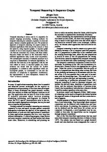
A finishes B B finished_by A A equals B Figure 2-1: The 13 relations between intervals in Allen’s algebra. Interval A is always either at the right or top of interval B. expression, at some time during the temporal expression, etc.). For a more detail discussion on reified logics see [Vila 1994]. Any TR formalism establishes a link between atemporal assertions and a temporal reference. The temporal reference is made up of a set of temporal elements related by one or more temporal relations. Different primitives have been considered for the temporal elements with main candidates time points, time intervals, or a combination of both. After deciding on the ontological primitive, one may want to give structure to this ontology by providing axioms describing the behavior of the temporal relations that we will call the structure of time. Some choices that have appeared in the literature are discrete vs. dense time, bounded vs. unbounded, and linear, branching, partially ordered, parallel, and circular precedence relations.
2.2.2 Constrained-based Temporal Algebras As mentioned in [Vidal 2000], in reified temporal logics the propositions are separated from their temporal qualifications. Queries such as “is proposition P true at time t?” are still processed at the logical level, but reasoning upon the temporal relations can be done through a purely temporal algebraic model. One usually gets a constraint network that is mainly used to check the temporal consistency of the given problem. In this thesis, we do not address the logic-based part of the temporal reasoning, but instead we tackle the algebraic, constraint-based, part of the reasoning. We can separate the temporal algebras and the constraint systems that have been developed into two large classes: qualitative and metric (also called quantitative). One of the first qualitative algebras was Allen’s algebra of intervals [Allen 1983]. It was based on the 13 mutually exclusive relations that can possibly exist between two intervals, as shown in Figure 2-1. In this algebra, time is linear and dense, and the time primitives are intervals. The constraints allowed between two time intervals A and B are of the form (A {r1 ∨ … ∨ rn } B) where ri is any of the 13 primitive relations. Each such constraint defines the possible relation between A and B, e.g. (A {meets, after} B) means that A either meets or is after B. Allen provides a polynomial time algorithm for computing the closure of a set of constraints that is sound but not complete. Kautz et al. [Vilain and Kautz
13
1986] proves that checking consistency in the interval algebra is NP-Hard. They thus suggest using a point algebra in which consistency checking under certain assumptions is polynomial. The point algebra is defined the same way the interval algebra is, but the elements are points and so there are only three simple point relations: precedes, equals, and follows. As expected, only a fragment of the interval algebra can be translated to the point algebra, namely all constraints that represent convex sets of intervals. Vilain and Kautz show that a constraint propagation algorithm excluding the relation (A {precedes ∨ follows} B) exists, with time complexity O(n3), where n is the number of time points. Later, Van Beek [Beek 1989] designed a O(n4) algorithm that includes this relation. This was later improved in [Meiri 1990] to O(n3). Other similar algebras include subsets of interval and point algebra so that the consistency problem becomes polynomial. For example NB [Nebel and Burckert 1995] is an algebra that admits only a subset of all the possible disjunctions that can be formed with the 13 basic relationships and that is polynomial, and actually the maximal subclass that contains all the 13 basic relationships. In quantitative temporal reasoning the constraints and temporal information can be metric. The simplest case is when this information is available in terms of specific dates or another precise numeric form and the durations and execution times of actions are absolute numeric values. Constant time algorithms can efficiently answer queries about occurrences by comparing these values. However, precise numeric information is not always available, in which case a constraint on the occurrence of an event E can be represented as an interval [lower-bound, upper-bound]. Similarly binary constraints between events take the form X – Y ∈ [l, u ], where X and Y are events (timepoints). This representation first appeared in [Dean and McDermott 1987] and then formalized and generalized in [Dechter, Meiri et al. 1991] by applying techniques from the Constraint Satisfaction Problem (CSP). This formalization was named Simple Temporal Problem (STP), while the generalization of the constraints X – Y ∈ [l, u ] to constraints of the form X – Y ∈ [l1 , u1 ] ∨ … ∨ [ln , un ] was named Temporal Constraint Satisfaction Problem (TCSP). The STP can be solved in polynomial time O(n3), where n is the number of time-points, by using all-pairs shortest paths algorithm, while there is no polynomial algorithm for the TCSP. The TCSP constraints can also be written as l1 ≤ X – Y ≤ u1 ∨ … ∨ ln ≤ X – Y ≤ un . A generalization of this kind of constraints is when we allow constraints of the form l1 ≤ X1 – Y1 ≤ u1 ∨ … ∨ ln ≤ Xn – Yn ≤ un , where the pairs Xi , Yi can be distinct in each disjunct thus allowing the encoding of non-binary constraints. This class of problems is the Disjunctive Temporal Problem first introduced in [Stergiou and Koubarakis 1998] and it is very expressive. Other types of problems include STPs with strict inequalities [Gerevini and Cristani 1997] (e.g. X < Y), STPs with inequalities (e.g. X ≠ Y) [Koubarakis 1992], STPs with conditional branches (CSTPs) [Tsamardinos, Pollack et al. 2000], and the temporal networks of Barber [Barber 2000], which extend TCSPs with forbidden non-binary assignments. This latter classes reaches the expressiveness of DTPs. Another important class of problems is the Simple Temporal Problem with Uncertainty (STPU) [Vidal and Ghallab 1996]. All the above classes of problems consider consistency as the existence of an assignment to the temporal variables that respects all the constraints (except CSTPs and CDTPs, as we will see at Chapter 6). The STPU however, distinguishes between time-points that are assigned times by the deliberative agent (called controllables), and those that are assigned time by other agents, Nature, or other uncontrollable procedures. With STPUs there are many 14
notions of consistency (which in STPU terminology is called controllability): for example, whether there is a way to assign times to the controllable events so that they respect the constraints no matter how the when uncontrollable events occur. We refer the reader to [Vila 1994; Gennari 1998; Schwalb 1998] for a more detailed discussion of all of the above temporal problems. For the purposes of this dissertation the most important class of problems are the DTPs, CSTPs, TCSPs, STPUs, and Barber’s temporal networks, which will be explained in more detail later in this section and at Chapter 6. An additional related area of research is that of Temporal Constraint Logic Programming, which involves embedding temporal models in the Constraint Logic Programming paradigm. Logic Programming in general is a class of languages in which information is described using “ifthen” rules of assertion. Each rule is of the form H:- B1 , …, Bn , where H is the head of the rule and B1 , …, Bn are atoms that constitute the body. Prolog is the most popular of this type of languages. Constraint Logic Programming began as a natural merger of the two paradigms of CSP and Logic Programming [Smith 1995]. The combination helps make Constraint Logic Programming programs both expressive and flexible, and in some cases, more efficient than other kinds of programs[Hentenrick 1989; Jaffar and Lassez 1994]. A CLP program is composed of rules of the form H : - B1 , …, Bn , C1 , …, Cm where again H is the head of the rule, B1 , …, Bn are the non-constraint atoms in the body of the rule, and C1 , …, Cm are the constraint atoms in the body of the rule. Note that constraint atoms cannot appear in the head of the rule. CLP programs differ from traditional logic programs in the way the constraint atoms are processed. In standard logic programming, the constraint and non-constraint atoms are treated equally. In CLP, specialized techniques for deciding which constraints are entailed, called constraint propagation algorithms, may be applied to the constraint atoms only. In Temporal Constraint Logic Programming the constraints allowed in the rules are temporal constraints. [Schwalb 1998] describes two such languages that combine the TCSP model to a couple of CLP languages. Our hope is that our DTP solving techniques of Chapter 4, like TCSP, will also find their way into Temporal Constraint Logic Programming languages.
2.3 The Simple Temporal Problem (STP) We now formally and technically discuss a particular constraint-based temporal reasoning formalism called the Simple Temporal Problem. A Simple Temporal Problem (STP) is a collection of variables V, each of which corresponds to a time point or instantaneous event, and a collection of constraints between the variables, C. The constrains are binary and each constraint between two variables X and Y is of the form Y – X ≤ bXY, where b is any real number and is called the bound of the constraint. The STP can be represented with a directed, weighted graph , where each edge E has an associated bound: for each constraint Y – X ≤ bXY in C there is an edge in E from X to Y with weight bXY. The corresponding graph or network is called a Simple Temporal Network or STN and the two terms STP and STN can be used interchangeably; similarly the term constraint and edge will be used interchangeably. Figure 2-2 displays an example STN. A pair of constraints Y – X ≤ bXY and X – Y ≤ bYX can be grouped together in one constraint -bYX ≤ Y – X ≤ bXY and be shown on an STN as an interval edge from X to Y with weight the interval [-bYX, bXY]. Intuitively such an edge can be
15
interpreted as the constraint that Y should only follow X after t time units, where t belongs in [bYX, bXY]. Figure 2-2(b) shows the original STN with its edges converted to interval edges. Interval edges are frequently used in the literature as an intuitive way to draw and display STNs. Definition 2-1: A Simple Temporal Problem (STP) is a directed edge-weighted graph where V is the set of temporal variables (nodes) and E the set of edges. The variables represent time-points and their domain is the set of reals ℜ (and so time is assumed dense). Each edge is labeled by a real value weight that is called the bound of the edge. The bound of the edge from node X to node Y is denoted as b XY and the edge as XY or (X, Y). Each edge XY imposes the following constraint on the values assigned to its end-points: Y – X ≤ bXY . The definition for STPs with edges annotated with an interval instead of a single bound is equivalent and we will use both interchangeably. Definition 2-2: Let N be an STP and V={p1, ...,pn} be its set of nodes. A tuple X=(x1, ..., xn) is called a solution iff the assignment { p1 = x1 ,..., p n = x n } satisfies all the constraints. The network N is consistent if and only if there is at least one solution. Two networks are equivalent if and only if they represent the same solution set. Let p be any path in an STN between two nodes X and Y. Path p imposes the following constraints on the pair of nodes: p1 − X ≤ b Xp1 p 2 − p1 ≤ b p1 p 2 M Y − p n ≤ b p nY
where the pi are the intermediate nodes in the path p from X to Y . By adding these inequalities, it is easy to see that p imposes (implies) the constraint:
Y − X ≤ ∑i =1 b pi pi+1 n
B
2
4 [1,2]
-1
A
3 -1
-2
D
A
5
[1,3]
B
D [4,5]
-4
C
C
(a)
(b) Figure 2-2: An example STP
16
[2,4]
where X=p1 and Y=pn. The tightest constraint between X and Y is obviously imposed by the shortest path between them. The weight of the shortest path is called the distance between the two nodes and is denoted as dXY. In a consistent STN, the distance dXY is the smallest real for which the constraint Y – X ≤ dXY holds in all solutions. The constraint Y – X ≤ dXY is an induced or implied constraint. Theorem 2-1: An STP is consistent iff for every i , dii ≥ 0 or equivalently, there are no negative cycles in the graph [Dechter, Meiri et al. 1991; Meiri 1992]. STPs have a very attractive property [Dechter, Meiri et al. 1991]: determining consistency is polynomial. All induced constraints between any pair of nodes X and Y, i.e. all distances, can be found by applying path-consistency (see Chapter 3), which is equivalent to running an all-pairs shortest paths algorithm on the graph [Cormen, Leiserson et al. 1990]. The network can then be solved (i.e. a consistent assignment to the variables can be found), without backtracking, in polynomial time. In [Chleq 1995; Cesta and Oddi 1996] two techniques for incrementally determining consistency in an STP are described. That is, given a consistent STP N and some additional constraints, the algorithms determine if the resulting STP N’ remains consistent, in time typically much less than what it would take another consistency checking algorithm running from scratch on N’. Definition 2-3: The distance array for an STP N = is the V × V array with elements ai j : ai j = dij , where dij is the distance between nodes i , j ∈ V. The array can be considered as representing a complete network where there is an edge (i, j) for every i , j ∈ V with bound bij = dij, called the distance graph of the STP. The terms distance array and distance graph will be used interchangeably. When we tighten the constraints between every pair of nodes X and Y of an STP so that the only admissible values for their difference Y – X are values that participate in some solution, then the STP is minimal. Formally: Definition 2-42: An STP N is minimal if for each (induced or explicit) constraint –bYX ≤ Y – X ≤ bXY and every t ∈ [–bYX , bXY] there is a solution s such that Ys – Xs = t , where Ys , Xs are the times assigned to Y and X respectively in s. Theorem 2-2: Given a consistent STP N the equivalent STP N’ induced by its distance graph is the minimal STP equivalent to N. (Theorem 2.3, page 21, [Gennari 1998]). Theorem 2-2 thus determines one way to calculate the minimal STP for a given STP N. Since the minimal STP is obviously unique, finding the minimal STP and the distance graph are equivalent operations. The theorem can also be used to construct a solution to the STP as follows: 1. Pick arbitrarily any time point X, and set X = v , where v is any arbitrary value (typically, X=TR, where TR is the time reference point defined below, and v=0) 2. Pick a node Y ∈ V , and assign time t to Y such that t ∈ [–dYX , d,XY] 3. Re-calculate the minimal STP propagating the constraint Y – X = t 2
Adopted from [Gennari 1998], Definition 1.0.4, page 8, for STPs.
17
4. Go to step 2 until all the nodes have been assigned a time. The algorithm is correct because (i) if the network is consistent there will always be a value in [– dYX , dXY] to assign in step 2, and (ii) by the theorem and the definition of the minimal STP, any value t ∈ [–dYX , dXY] can be extended to a solution. As we will see in the next subsection, STPs can be used to represent the constraints of temporal plans. When such a plan is executed (equivalently, its STP is executed), times are assigned to the nodes of the STP (in which case we say that they are executed), effectively dynamically constructing a solution to the STP. The above algorithm for constructing a solution requires the propagation of a constraint in step 3 each time a node is executed. When systems have to execute temporal plans under strict real-time constraints, it is uncertain how much time this propagation will require. In [Muscettola, Morris et al. 1998; Tsamardinos 1998; Tsamardinos, Morris et al. 1998] an STP is reformulated to an equivalent one such that step 3 in the algorithm above provably requires the minimum propagation. In particular, this reformulated equivalent STP has the minimal number of edges with the property that propagation of execution constraints at step 3 only needs to be propagated to the immediate neighbors of the executed node. This line of work on dispatching and executing temporal networks is reviewed again and extended for DTPs at Chapter 5. Apart from representing and executing temporal plans, STPs can also be used to represent more general temporal information and can provide answers to the following types of queries: [0, 12] GB(?cb)S
GB(?cb)E
PCS
PCE
RB(?cb)S
RB(?cb)E
[4,∞]
TR GB(?lb)S
GB(?lb)E
PLS
[1,2] PLE
RB(?lb)S
RB(?lb)E
Figure 2-3: The STN for the painting example with additional constraints
• •
Is the information consistent? The answer is yes, if and only if, the corresponding STP is consistent. What is the allowable separation in the time between two events X and Y? The answer is Y can follow X by t time units, where t ∈ [-dXY, dYX ].
2.3.1 Using STPs to encode plans with quantitative temporal constraints We consider a plan as consisting of at least a set of steps S and a set of temporal constraints C among the steps in S. A plan might contain other objects too, but sets S and C are what is minimally required for out purposes in this section. We construct an STP to represent a temporal plan in the following manner: For each step A in the plan, the nodes AS and AE are inserted in an STP; these correspond to the events of starting and ending the execution of the action respectively. To be able to encode absolute time constraints such as “the start of step A is at
18
9:00am, this Monday”, a special node TR (the time reference point) is inserted in the STP that represents the plan, and is arbitrarily related to a date and time, such as 12:00am 1/1/2000. All other time points of the STP should be constrained to occur after TR. An STP can represent the temporal aspects of a plan only if the constraints in C can be encoded by STP-like constraints, thus, for example, disjunctive constraints are not included. We will now present an example (taken from [Yang 1997]): Figure 2-4 displays a plan for painting the ceiling and painting the ladder. There are eight steps in the plan, with Initial-State and Goal-State corresponding to two dummy steps of starting and ending the plan. All arrows indicate ordering constraints constraining the action at the end of the arrow to succeed the one at the beginning of the arrow. The argument to steps Get-Brush and Return-Brush is a paintbrush. In addition to the ordering constraints shown in Figure 2-2 let us assume that the temporal constraints should also hold: • Painting the ceiling should end by 12:00pm 1/1/2000. • Painting the ladder takes between 1 and 2 hours. • Getting the ceiling brush (Get-Brush(?cb)) should occur at least 4 hours after (finishing) getting the ladder brush (Get-Brush(?lb)) The resulting STP that corresponds to the plan with the addition of the temporal constraints is shown at Figure 2-3, where TR is assumed to be 12:00am 1/1/2000. For readability, the interval annotation for all edges is omitted when it is [0, +∞], time units are assumed hours, and instead of the whole action name, only the acronym is used. The two dummy steps are also omitted from the figure.
Getbrush(?cb)
PaintCeiling
ReturnBrush(?cb)
Initial State
Goal State Getbrush(?lb)
PaintLadder
ReturnBrush(?lb)
Figure 2-4: A simple temporal plan for painting a ladder and the ceiling
2.4 The Temporal Constraint Satisfaction Problem (TCSP) A Temporal Constraint Satisfaction Problem (TCSP) [Dechter, Meiri et al. 1991] is a generalization of the STP. Definition 2-5: A Temporal Constraint Satisfaction Problem (TCSP) is a directed edge-weighted graph where V is the set of temporal variables (nodes) and E the set of edges. The nodes represent time-points and their domain is the set of reals ℜ. Each edge XY is labeled by a set of intervals I1 = [l1 , u1], …, In = [l1 , ln ] and corresponds to the constraint: 19
[0, 1] [1, 2] [16, 17] [11, 12] [23, 24] [21, 22] [0, 22][23, 33][34, 50]
[0, 1] [1, 2] [16, 17] [11, 12] [23, 24] [21, 22] [1, 3] [11, 13][17, 19] [21, 22] [23, 23] [24, 26] [27, 29] [34, 36] [44, 46]
Figure 2-5: A TCSP and its minimal TCSP
l1 ≤ Y − X ≤ u1 Kl n ≤ Y − X ≤ u n or equivalently Y – X ∈ ∪i Ii The definitions for the solution of a TCSP, TCSP consistency, and equivalent TCSPs are generalizations of the corresponding definitions for STPs. Notice than an STP is a TCSP where all edges are annotated with one interval. By selecting one interval Ii from each edge we form a component STP. The consistency of the STP can be determined in polynomial time and if there is a consistent component STP then the TCSP is also consistent since any solution of the STP is also a solution of the TCSP. Conversely, if there is no consistent projected STP, the TCSP is inconsistent. Unfortunately, there is an exponential number of possible component STPs in any TCSP and thus the problem of solving the TCSP is NP-Hard. This is proven by reduction to the 3-coloring problem in [Dechter, Meiri et al. 1991]: Theorem 2-3: Consistency checking in TCSP is NP-Hard. Similar to the minimal STP of a given STP, we can define the minimal TCSP as follows. Definition 2-6: An TCSP N is minimal if for each (induced or explicit) constraint Y – X ∈ ∪i Ii and every t ∈ ∪i Ii there is a solution s such that Ys – Xs = t , where Ys , Xs are the times assigned to Y and X respectively in s. The minimal TCSP is unique for a given TCSP (see page 19, [Gennari 1998]) but unfortunately the problem of calculating the minimal TCSP is exponential because of fragmentation: that is the number of intervals in the minimal TCSP is exponential to the number of intervals on the edges of the original TCSP (see Figure 2-5 for an example taken from [Schwalb 1998]). For state of the art algorithms on solving TCSPs see [Schwalb 1998]. Running a path-consistency algorithm on the network approximates calculating the minimal TCSP. A path-consistency algorithm is sound but incomplete, meaning that it can sometimes correctly determine that a TCSP is inconsistent, but it will not always identify a TCSP as inconsistent if this is the case. A complete algorithm for determining consistency requires backtracking search, meaning incrementally selecting one interval from each edge, thus gradually building a consistent component STP. When the search reaches a dead-end and there is no way to select an interval from an edge in any consistent way with the current STP, the search backtracks to alter a previous choice of an interval. In addition, Schwalb [Schwalb 1998] suggests that every time we select an interval from an edge to extend the currently built component STP, we propagate this decision by running path-consistency and tighten the values on the un-instantiated
20
edges. Schwalb suggests two looser types of path-consistency that avoid the fragmentation problem (but they do not have the pruning power of the full path consistency) and reports significant performance improvements.
2.5 The Simple Temporal Problem with Uncertainty (STPU) The Simple Temporal Problem with Uncertainty (STPU) model extends the STP by taking into account the uncertain nature of durations of some tasks. It distinguishes between contingent constraints whose effective duration is observed only at execution time, and controllable ones, whose instantiation is controlled by the agent [Vidal 2000]. This contrasts the STP, TCSP, and most other such models that assume that times can be assigned to the variables (nodes) at will by the agent. In planning applications when these models encode temporal plans, some events are inherently uncontrollable and this is exactly what the STPU model is trying to take into account. In [Vidal and Morris 2001] an STPU is defined as follows: Definition 2-7: A Simple Temporal Problem with Uncertainty (STPU) is a tuple , where V is a set of temporal variables (nodes), E a set of edges between the nodes associated with an interval [l , u ], and C ⊆ E, called contingent edges or contingent links, and each edge XY imposes the constraint l ≤ Y – X ≤ u (equivalently Y – X ∈ [l, u]) . It is also required that for each contingent link with the interval [l, u], 0 < l < u . The non-contingent links are called requirement links and when the distinction between contingent and requirement links is dropped it is easy to see that we end up with an STP. The semantics of an STPU is that it is Nature, or some other uncontrollable agent, that will instantiate the value of Y for every contingent link XY, respecting the constraint of the contingent link l ≤ Y – X ≤ u. Equivalently, Nature will pick the value t so that t = Y – X ∈ [l, u], given the value the agent assigned to X. For example if X is a node that corresponds to starting an action A and Y corresponds to the event of ending the action A, and we know that A will take between 3 and 5 time units, we can model this fact with the contingent link Y – X ∈ [3, 5]. During execution, if action A starts at time unit 10, i.e. X=10, Nature will assign a time to Y so that Y – X ∈ [3, 5], in other words Y can be anything in the interval [13, 15]. This distinction between contingent and requirement links gives rise to three notions of consistency, which for STPUs is instead called controllability. Each notion is appropriate in a different execution situation. Before we define them, we need to first defined the following concepts [Vidal and Morris 2001]: Definition 2-8: A projection of an STPU Γ is an STP derived from Γ by replacing each requirement link by an identical STP edge, and each contingent link XY with interval [l , u] by an STP link with equal lower and upper bounds [b, b] for some b such that l ≤ b ≤ l. . Definition 2-9: Given an STPU Γ a schedule T is a mapping T: N →ℜ , where T(x), x ∈ V is called the time of time-point x. A schedule is consistent if it satisfies all the link constraints. From a schedule, we can determine the durations of all contingent links that finish prior to a time-point x. We will call this the prehistory of x with respect to T, denoted by T 15, implying that only triplets of values whose total is more than 15 are valid. Definition 3-2: For the CSP , a CSP assignment {v1 ← d1 , …, vn ← dn} (partial or complete) of the variables vi ∈ V, where di ∈ D(vi) violates a constraint Cj ∈ C if it is a superset of Cj . An assignment is consistent if it does not violate any constraint in C. A complete and consistent assignment is called a solution. If there is a solution to a CSP then it is called consistent.. Definition 3-3: A unary constraint is an illegal assignment that involves only one variable. A binary constraint is an illegal assignment that involves two variables. A binary CSP is one in which each constraint is unary or binary. An n-ary CSP is one in which the arity of some constraints is greater than two.
More often, in the definition of CSPs, the constraints are defined as subsets of allowable assignments. Obviously, the two definitions are equivalent. The reason for departing from the standard definition is that constraints defined our way are the same as no-good assignments that will be used for no-good learning. 3
23
Example 3-1: Let V = {a, b, c}, D(a)=D(b)=D(c)={1, 2} and C = {C1 ={a ←1, b ←2}, C2 ={a ←2, c ←2}, C3 ={b ←2, c ←2}, C4 ={a ←1, c ←1}, C5 ={a ←1, c ←2}}. There are three variables, five constraints, and two values in each variable domain. One solution to this CSP is {a ←2, b ←1, c ←1} and thus the CSP is consistent. The assignment {a ←2, b ←1} is not a solution because it is not a complete assignment, while the assignment {a ←2, b ←1, c ←2} is not a solution because it violates the constraint C2 = {a ←2, c ←2}. Typical examples of problems that map to CSPs are the N-Queens problem [Minton, Johnston et al. 1990], the SAT problem [Du, Gu et al. 1997], and the graph-coloring problem [Yang 1997] p. 58. In the N-Queens problem we seek an assignment of N queens on an N×N chessboard, in such a way that no queen threatens any other queen. There are various ways to represent this problem as a CSP and numerous studies have demonstrated the implications of alternative representations on solution efficiency. In one typical representation there are n variables vi , I=1,…,n each with domain set {1, … , N} representing the column (or row) to assign to the queen. In the final solution, each queen will be placed at position (i, vi). The constraints in the CSP allow only placements in which the queens do not threaten each other. In the SAT problem we seek for a truth assignment to a set of variables so that a propositional logic formula over those variables is satisfied. If the formula is in Conjunctive Normal Form, each clause forms a constraint to be satisfied in a CSP problem in which the variables correspond to the variables in the logic formula. Finally, in the graph-coloring problem, we would like to color each vertex of a graph with a different color than any other vertex connected to. Each vertex to be colored forms a variable in a corresponding CSP, each possible color for the vertex, a value in its domain, and each arc between vertexes induce a constraint specifying that the colors for the two vertexes should be different.
3.2 Solving Constraint Satisfaction Problems The literature on solving CSPs is vast and for the most part considers binary CSPs. In general, CSPs are solved by search and deduction or a combination of the two. In addition, there are two types of searches, systematic search and stochastic (local) search. Chronological backtracking is an example of systematic search (shown below). As the name implies, systematic search searches the whole space of possible assignments either explicitly or implicitly. Research in this area consists of finding algorithms that do not repeat unnecessary search effort with the least possible amount of bookkeeping. Some of these algorithms are Dynamic Backtracking [Ginsberg 1993], Conflict Directed Backjumping (CDB) [Prosser 1993; Chen and Beek 2001] and no-good recording [Dechter 1990], all described in detail in the survey paper [Dechter and Frost 1999]. Stochastic search methods move in a hill-climbing manner in the space of complete instantiations. The disadvantage of this kind of approach is that it does not report an inconsistency if the problem has no solution and this is the reason they will not be considered in this dissertation4. A generate-and-test is a very simple search method that could be used to solve CSPs. Each possible assignment is first generated and then tested against each constraint to ensure it does not 4
There are some exceptions to the rule however (see [Ginsberg and McAllester 1994]).
24
violate it. A slightly more intelligent approach is to use a backtracking Depth-First search. During search an assignment for the variables is built incrementally. As soon as the current assignment violates a constraint there is no need to keep extending it, as every extension will still violate the same constraint. Therefore, the search underneath that subtree is stopped and the search tries a different value for the last variable. When all values of the last variable have been tried, the search backtracks to the previous variable. This kind of search is also called chronological backtracking. Finding one solution to the CSP of Example 3-1 is shown at Figure 3-1. At the bottom of each leaf representing an inconsistent assignment, one constraint that is violated by the leaf’s assignment is shown. In this dissertation, we will only concern ourselves with finding one solution to a CSP or proving the CSP has no solutions, and we will not be concerned with the problem of finding all solutions of a CSP, even though most times extending the algorithms to report all solutions is trivial (see [Chen and Beek 2001] pp. 59-60 for extending CDB to find all solutions). In general, finding a solution to a CSP is NP-complete. Deduction in the CSP framework is known as constraint propagation or consistency enforcing. Deduction algorithms reason with constraints to prune out inconsistent values or partial assignments either before start searching for a solution, i.e. as a preprocessing step, or during search. The better known of these techniques include node-consistency, arc-consistency, and path-consistency [Montanari 1974; Mackworth 1977; Tsang 1993]. A CSP is k-consistent iff given
{} {a ← 1}
{a ← 2}
{a ← 1, b ← 1}
{a ← 1, b ← 2}
{a ← 2, b ← 1}
C1 {a ← 1, b ← 1, c ← 1} C4
{a ← 1, b ← 1, c ← 2}
{a ← 2, b ← 1, c ← 1}
C5
Solution!
Figure 3-1: Chronological search for solving the CSP of Example 3-1. any consistent partial instantiation of any k –1 variables, there exists a consistent instantiation of any kth additional variable. For binary CSPs, the terms node-, arc-, and path-consistency correspond to 1-, 2-, and 3-consistency respectively.
25
Structure-driven algorithms, which attempt to characterize the topology of constraint problems that are tractable, take advantage of the special structure of some CSP problems, or transform general CSPs to CSPs with special topology that makes it easy for algorithms to solve. Structuredriven algorithms will also be not considered in this dissertation because they depend on the special structure of problems, and there is no indication that the CSP-type problems we will be considering have any special structure or could be easily converted to problems with special structure. In particular when converting a DTP to a meta-CSP (explained later), the constraints are neither binary (a typical assumption of structure-driven algorithms; see [Bessiere 1999] for a discussion on the thesis that non-binary constraints have not achieved enough focus in the literature) nor they are represented explicitly (instead they are discovered during search). It is not obvious how structure-driven algorithms could be extended to take into account implicit constraints.
3.3 A Theory of No-goods This section illustrates the concept of no-goods [Dechter 1990; Frost and Dechter 1994; Ginsberg and McAllester 1994; Schiex and Verfaillie 1994; Schiex and Verfaillie 1994; Yokoo 1994; Dechter and Frost 1999], which is an advanced and powerful tool in solving CSPs and Dynamic CSPs (to be introduced later). Definition 3-4: A constraint A is induced by a CSP if it is satisfied (not violated) in all the CSP solutions. Let A ↓ V denote the assignment that results from projecting assignment A on the variables of V. For example, if A = {a ←2, b ←1, c ←2} and V = {a, c} then A ↓ V = {a ←2, c ←2}. In addition, let CV ∈ C be the constraints in C that involve only the variables in V, and VC. be the variables in V that appear in the constraints in C. Definition 3-5: A no-good of the CSP is a pair , where A is an assignment of values to a subset of V, and J ⊆ V such that no solution of the CSP contains A. Stated otherwise, the constraint forbidding A is induced by the CSP . The set J is called the no-good justification (or culprit). Example 3-2: Consider again the CSP of Example 3-1 restated here for clarity: V = {a, b, c}, D(a) = D(b) = D(c) = {1, 2} and C = {C1 ={a ←1, b ←2}, C2 ={a ←2, c ←2}, C3 ={b ←2, c ←2}, C4 ={a ←1, c ←1}, C5 ={a ←1, c ←2}}. Each constraint Ci trivially defines a no-good: For example, C1 implies that is a no-good. Now notice that when a ←1 constraint C4 precludes c from taking value 1 and C5 precludes c from taking value 2 either. Since these are the only values in the domain of c , D(c), we can infer that a ←1 is an induced constraint. Thus, the pair , where A={a ←1}, is a no-good. What is the justification J? The constraints that imply the no-good are C4 and C5. Thus, the variables that “justify” the no-good are the variables of these two constraints and so J = {a, c}. CJ = {C2 , C4 , C5} and, as the definition requires, the CSP implies that A cannot
26
be contained in any solution of it5. Notice at this point, that a no-good does not only depend on the constraints C of the CSP, but also on the domains in D. If the domain of c in this example contained more values than 1 and 2 we could not have inferred A={a ←1} is an induced constraint. Theorem 3-1: Let be a no-good, and be such that J ⊆ J’ and A ⊆ A’ (noted as ≤ ). Then < A′ , J′> is a no-good. (Theorem 3.1 in [Schiex and Verfaillie 1994], page 5) Example 3-3: We will use again the CSP of Example 3-2 to illustrate the theorem. We showed that is a no-good. By the theorem, , , and are all no-goods too. Obviously, ≤-minimal no-goods are preferred since they implicitly define more no-goods according to Theorem 3-1. Theorem 3-2: Let be a no-good, then is a no-good (theorem 3.2 in [Schiex and Verfaillie 1994], page 5). Intuitively, the theorem states that we can reduce the assignment of a no-good, by only considering the variables in the justification. For example, if is a no-good, then = is also a no-good. Theorem 3-3: Let A be a (partial) assignment of the variables in V, vs be an unassigned variable in V, and {A1 , …, Am} be all the possible extensions of A along vs , using every possible value of D(vs) . If , …, are no-goods, then
is a nogood (corollary 3.1 in [Schiex and Verfaillie 1994], page 5) Example 3-4: Theorem 3-3 is exactly what we used intuitively in Example 3-2 to infer that is a no-good. Let us illustrate now the same CSP and the same derivation again in light of Theorem 3-3. If we let A = {a ←1}, we see that A1 ={a ←1, c ←1} and A2 = {a ←1, c ←2} are all the possible extensions of A along variable c. Trivially (see the discussion in Example 3-2), and are no-goods, or equivalently and are no-goods. By the theorem we infer that . Theorem 3-2 and Theorem 3-3 will be the main tools in building smaller and smaller no-goods during search in a never ending attempt to reduce the required search.
3.4 A No-good Learning Algorithm This section presents a no-good learning algorithm published in [Schiex and Verfaillie 1994]. The algorithm utilizes Theorem 3-2 and Theorem 3-3 to successively build smaller and smaller nogoods from previously identified ones and is presented in Figure 3-2. The top procedure (line 1) NR should be called with a partial assignment A and the set of still unassigned variables U. So, for any CSP , the initial call to NR should then be NR(∅, V). If a solution is found to the CSP by NR it is reported at line 3, otherwise a justification J for the failure of an extension to assignment A is returned. The justification J is the same as a no-good justification: a set of variables whose interrelated constraints are responsible for the failure to extend the assignment A. In other words, if NR(A, U) returns J then is a no-good. During the search and the recursive calls, NR records the no-goods it discovers and uses them to prune the search space. Let us trace the algorithm in Figure 3-2. If there are no more variables to assign, that is U=∅, then the assignment A is a solution and so we and stop and report it (line 2). Otherwise, a variable x is chosen by function select-variable from the unassigned variables to be assigned a value (line 5). At line 6, all possible values v to x are assigned in turn. The function backward-check called with an assignment A’ tests whether A’ violates an existing (explicitly given) constraint or a recorded no-good, in other words if it is inconsistent. If A’ is consistent, backward-check returns the empty set. If not, it returns a justification that depends on the kind of the failure: if a recorded no-good is a superset of A’ then the returned justification is J . If on the other hand, an explicit constraint Ci is violated the justification returned is the variables that appear in the violated constraint Ci . There are three distinct paths of execution in the code in Figure 3-2: 1. K = ∅ and x ∈ J-sons 2. K = ∅ and x ∉ J-sons 3. K not equal to ∅ We will show that no matter what path of execution is followed in any loop iteration, NR will return the correct justification. Let us assume for a moment that in every loop iteration only case (3) occurs, i.e. every extension of A in the call of NR along the variable x violates some induced or explicit constraint (and so the code never enters line 10). Let us denote with vm the value of variable v in the figure above at the mth iteration of the loop at line 6. Then, as described above, backward-check returns a justification Km so that is a no-good. By Theorem 3-3 is a no-good and the justification ∪m Km is exactly what is stored at variable J in line 18, recorded in line 21, and eventually returned, in line 22. Let us relax now the assumption that in every iteration we fall into case (3) and assume that we either fall into case (3) or (1). Whenever we fall into case (1) then NR is called recursively at line 10. If it ever returns, then because of line 3, a solution has not been found. NR will return with the justification of the failure J-sons which implies that is a no-good. As before is a no-good where J=∪m Jm ∪r J-sonsr is the variable returned at line 22.
28
Finally, if in any iteration we fall into case (2) then we stop iterating (by setting BJ to True) and return J = J-sons. Stopping the iteration means that we are not trying any other values for x. Let us assume that we do not distinguish this case from when x is involved in J-sonsk (case 1). Then, the next iteration of the loop will assign a different value to x and so the recursive call to NR will be with the assignment A ∪ {x ← vm+1}. Since x is not involved in the justification J-sonsk that means that changing its value will have no effect to the recursive call which will return again with a failure and the same justification. Since trying different values for x has no effect, we can backjump variable x without trying the rest of its values. This is why the algorithm at line 14 handles 1. NR(A, U) 2. If U=∅ Then 3. A is a solution, Stop and report A. 4. Else 5. x = select-variable(U), J =∅, BJ = false 6. For each v ∈D(v) until BJ 7. A’ = A ∪ {x ← v }, 8. K = backward-check(A’) 9. If K = ∅ ;; That is, A can be extended along x 10. J-sons = NR(A’ , U – {x} ) 11. If x ∈ J-sons Then 12. J = J ∪ J-sons 13. Else 14. J =J-sons 15. BJ=true 16. Endif 17. Else 18. J=J∪K 19. Endif 20. EndFor 21. If BJ = false then record(project(A, J), J) Endif 22. Return J 23. Endif Figure 3-2: The no-good recording algorithm differently this case and sets BJ to be True so that we exit the loop and return from the call to NR. This type of backjumping is closely related to conflict-directed backjumping (CDB) proposed in [Prosser 1993] . The actual no-good recording occurs at line 21. As already mentioned, J contains the justification why is a no-good, but from Theorem 3-2 we also know that is also a (potentially smaller) no-good and so it is preferable to record the latter one. Function project (A, J) returns A ↓ J and function record(A, J) records the no-good . Notice, that if
29
we have to backjump and so BJ is true, then there is no need to record the no-good. It will have already been recorded at the recursive call to NB. The algorithm is proved to be sound, complete, and terminating at [Schiex and Verfaillie 1994].
3.4.1 An example run of the no-good learning algorithm This subsection presents an example taken from [Schiex and Verfaillie 1994] to clarify the workings of the algorithm in Figure 3-2. The algorithm will run on the problem presented at Figure 3-3. In the CSP of the figure there are five variables x1-x5 corresponding to each circle with domains as given. The constraints among the variables are binary. For example, the edge from x1 to x3 represents the constraining assignments between these two variables, shown beside it. All the ordered pairs of values in the array are forbidden assignments, e.g. { X1 ← a , X3 ← a} is a constraint. Calling the function NR of Figure 3-2 and using the variable ordering (x1 , x2 , x3 , x4 , x5) will create the search tree of Figure 3-4. Simple chronological backtracking algorithm explores the full tree while the NR algorithm only expands the bold edges. The no-goods built and recorded are given inside the ovals with a dotted arrow giving the nodes where they have been built (trivial no-goods corresponding to each leaf marked with × are not shown in the figure as they are not recorded). Let us see how the first recorded no-good is built: 1. the assignment A1 = {x1 ← a, x2 ← a , x3 ← a} is inconsistent because it violates the constraint {x2 ← a , x3 ← a} (check the array by the edge x3 to x2 at Figure 3-4. Trivially then is a no-good and function backward-check at line 7 returns {x2 , x3}. 2. in the next loop iteration, the assignment A2 = {x1 ← a, x2 ← a , x3 ← b} violates again a constraint between variables x2 and x3 and again is a no-good and backward-check returns {x2 , x3}. 3. it is now possible to apply Theorem 3-3 (line 21) and infer that < {x1 ← a, x2 ← a }, {x2, x3 }> is a no-good. Before recorded however, the call to project (line 21 again) reduces the no-good to . One may notice that the empty 0-ary constraint is induced last. This constraint simply states that the CSP is inconsistent and its justification {x3 , x4 , x5} is a minimal justification of the CSP inconsistency.
30
X2
{a, b, c}
{a, b, c}
X1-X3 (a a) (a b) (b b)
X2-X3 (a a) (a b) (b b)
X3
X3-X5 (a a) (b a) (b b)
{a, b} X3-X4 (a a) (b a) (b b)
X4
X5 X4-X5 (a a) (b a) (b b)
{a, b}
{a, b}
Figure 3-3: An example CSP
b
a
c
X1 X2
a
b
c
a
b
c
a
b
c
X3 a× b× a× ×b a× b×
a× b× a b× a b×
N ( X , ¬A} In English, the above formula says that Y can occur before X in all scenarios, in which case Y has to be synchronized between scenarios, or Y should occur after X in all scenarios. The above formula can be simplified as: {( N (Y , A) ≤ N ( X , A) ∧ sync (Y , A, ¬A) ∨ {( N (Y , A) > N ( X , A) ∧ N (Y , ¬A) > N ( X , ¬A)} [40,40] [20,20]
TR [0,0]
TR
X
Y
[10,10]
Α W
Z
[40,40] [20,20]
TR [0,0]
[0,0]
X
Y
[10,10]
Z
TR [30,30]
X [0,0]
X
Y [0,0]
Y
[10,10]
Α W
Z
[0,0]
[10,10]
V
Z [30,30]
¬Α
V
¬Α
[60,60]
[60,60]
(a)
(b)
Figure 6-16: The projection STPs with synchronization constraints We will call such constraints DC constraints (from Dynamic Consistency). Since DC constraints contain disjunctions, the translation method will result in general to a DTP and not an STP. If there is a solution to the resulting DTP, then the original CSTP is Dynamically Consistent. The problem that arises is how to formalize DC constraints and how to precisely state when they occur.
140
6.6.1 The problem with unordered observations A particularly difficult case is when CSTP observation nodes are unordered with respect to each other. For example, if O(A) and O(B) are unordered with respect to each other, then if O(A) occurs first we should synchronize CSTP nodes with label True if they occur before O(A), otherwise we should synchronize them if they occur before O(B). We know proceed with an example. Suppose we have a CSTP with two observations A and B unordered with respect to each other as shown in Figure 6-17, where O(A) = X and O(B) = Y . The exact structure of the network and number of nodes is irrelevant for our purposes and so there might be other nodes in
AB
Z A¬B
X TR
W ¬AB
Y
V ¬A¬B
U Figure 6-17: A CSTP unordered observations
with
CSTP not shown in the figure. There are four different scenarios for the CSTP, s1 =AB, s2 = A¬B, s3 =¬AB , s4 = ¬A¬B The projected STPs when O(A) < O(B) are shown in Figure 6-18(a) and when O(B) < O(A) in Figure 6-18 (b). All the arrowed edges are ordering constraints [0, ∞] and all non-arrowed edges are synchronization constraints [0, 0]. The scenario of each projected STP is shown at the right side of it. In Figure 6-18 (a) the constraint X < Y is not in the original CSTP, but we display it in the figure because we assumed that O(A)=X < O(B)=Y . What conclusions can we draw from this situation? First of all, after we observe both A and B, i.e. both X and Y are executed, we know exactly which scenario we fall into and we can make an independent decision for any N(v, s) for any node v that comes after X and Y and any scenario s, i.e. we do not need to synchronize v in any scenario. More specifically, this means that any node after Y in the figure 6-20(a) and any node after X in figure 6-20(b) does not have to be synchronized. For any node v that appears in all scenarios before either observation, we have no information about which scenario we will be following, and thus v has to be synchronized in all scenarios. This is the case for TR in both figures and for X in figure 6-20(a) and Y in figure 620(b).
141
Between these two extremes of not synchronizing in any scenario and synchronizing in all scenarios, there are intermediate situations. In figure 6-20(a), after we observe A by executing X we know whether A is True and thus we know we will fall in one of {s1 , s2 } or {s3 , s4 }, but we still do not know with certainty the exact scenario. Thus, in figure 6-20(a) we need to make a common decision about the time we execute Y for both scenarios {s1 , s2 } and a common decision for Y for scenarios {s3 , s4 }. This is why there are the synchronization constraints sync(Y , s1 , s2) and sync(Y , s1 , s2) (in the figure shown as solid arrows between the corresponding nodes). In a
TR
X
Y
Z
s1=AB
TR
Y
X
Z
s1=AB
TR
X
Y
W
s2=A¬B
TR
Y
X
V
s3=¬AB
TR
X
Y
V
s3=¬AB
TR
Y
X
W
s2=A¬B
TR
X
Y (a)
U
s4=¬A¬B
TR
Y
X (b)
U
s4=¬A¬B
Figure 6-18: The STP projections of the CSTP of Figure 6-17 similar fashion we can see that in when B is observed first as in figure 6-20(b), we have to add the synchronization constrains sync(X , s1 , s3) and sync(X , s2 , s4). Let us suppose now that the CSTP presented in the example has one more node R with label True that is underconstrained and can potentially occur in any order relatively to X, Y, Z, W, V and U (but it has to occur after TR). What constraints added to the union of the projected STPs will enforce that a solution to the “super”-STP will guarantee the correct execution of the CSTP under any outcome of the observations? It is either the case that (i) O(A) = X < O(B)=Y or (ii) O(B)=Y < O(A) = X (we are ignoring the equality case for the moment). If (i) then if R is scheduled between TR and X it should be synchronized between all scenarios, else if it falls between X and Y is should be synchronized between {s1 , s2 } and {s3 , s4 }, else if it falls after Y it should not be synchronized in any scenario. If (ii) holds instead then similar constrains should be added. We can express these constraints just expressed in English using disjunctions and conjunctions of STP-like temporal constraints. Let us now summarize the conclusions from this section. The main idea is that we can take the projected STPs for each (minimal) execution scenarios, add temporal constraints among them (disjunctive ones in the worst case, STP-like ones in the best case) and transform the problem to a large DTP problem. The super-DTP will have a solution if and only if the original CSTP is Dynamically Consistent. Moreover, we saw that, for a fixed order of the observation nodes, if a node v is executed in two scenarios before we have enough information to distinguish between the two scenarios, we have to synchronize it. For nodes that can “float” around and that are allowed to be executed either before we can distinguish between the two scenarios or after, we have to add a disjunctive constraint called DC that synchronizes the node in the pair of scenarios if we decide to schedule the node before the distinguishing node, or imposes the constraint that the node is executed after this distinguishing point in both scenarios.
142
Finally, this last subsection in particular, was devoted to the importance of ordering the observation nodes. If observation nodes are unordered with respect to each other, then the constraints that we have to add for one particular order may differ significantly from when we execute these nodes in a different order. Unfortunately, it is our intuition that we have to deal individually with each order of the observation nodes that is allowed by the constraints. For P number of propositions this gives a worst case of P ! possible orderings in the worst case. And for each one such ordering a large number (in the worst case) of disjunctive constraints needs to be added. Thus, in the worst case determining Dynamic Consistency is very hard to compute, even though we do not prove any theoretical result such that the problem is NP-complete.
6.7 Checking Dynamic Consistency This section provides a general Dynamic Consistency checking algorithm and proves it is correct. The algorithm is exponential in the worst case in the number of propositions and nodes in the CSTP. Here the first algorithm that solves the problem is presented. Our intention here is to focus more in the clarity of the algorithm and ease of proving correctness despite its computational inefficiency. After the general result, we investigate special cases where additional structural assumptions are imposed on the CSTP, resulting in computationally more efficient consistency checking algorithms. We begin by formalizing the discussion in section 6.6. Let us assume a total order of the observations order and consider a node v that appears in both scenarios s1 and s2 (for a node that appears in only one scenario there is no need for the addition of any kind of constraint). In addition, let O(A) be the distinguishing observation, i.e. O(A)= Dis(s1 , s2 , order). Trivially, we can infer that O(A) has to be synchronized in the two scenarios: by definition this is the earliest time at which we can distinguish between the two scenarios.. Thus, we should impose the constraint sync(O(A), s1 , s2 ) and since N(A, s1) = N(A, s2) we can just define N(A, s1) = O(A) . Then for any other node v we can distinguish among the following cases: 1. N(v , s1) < O(A) or N(v, s2) < O(A) If at least one of N(v , s1) and N(v, s2) has to be executed before O(A) then they must be synchronized and must both be executed before O(A).We add the constraint: sync(v, s1 , s2 ). 2. N(v , s1) > O(A) or N(v, s2) > O(A) Similarly, if at least one of N(v , s1) and N(v, s2) has to be executed after O(A), they must both be executed after O(A). In this case however, we will know if we are falling into s1 or s2 and we can make a different decision for N(v , s1) and N(v , s2), i.e. v is left unsynchronized. So we should impose the constraints: N(v , s1) > O(A) and N(v, s2) > O(A) 3. N(v , s1) O(A) and N(v, s2) O(A)22
22
We use to denote that the left hand side is unordered with the right hand side.
143
GeneralDynamicConsistency(CSTP Cstp) 1. D = GeneralTranslateCSTP2DTP(Cstp) 2. Solve D by using DTP consistency checking algorithms 3. If D is consistent, return Dynamic-Consistent, otherwise return not-Dynamic-Consistent GeneralTranslateCSTP2DTP(CSTP Cstp) 4. DTP D = , where Pr(si) = are the projected STPs 5. For each allowable order order = O(p1) ≤ …≤ O(pn) of the observations in Cstp 6. For each pair of scenarios s1 and s2 7. For each node v that appears in both s1 and s2 8. NewCv, s1, s2= the constraint returned by cases 1, 2, and 3 above 9. C = C ∪ {order ⇒ NewCv, s1, s2} 10. EndFor 11. EndFor 12. EndFor 14. Return D Figure 6-19: The algorithm for determining Dynamic Consistency in the general case. In this case, we can decide to either execute v before O(A) – in which case we have to synchronize it – or execute it after and leave it unsynchronized. So, we should impose the constraint: { N(v , s1) < O(A) and sync(v, s1 , s2)} or { N(v , s1) > O(A) and N(v, s2) > O(A)}23 Putting all of our conclusions in use, we present a Dynamic Consistency checking algorithm in Figure 6-19. The algorithm translates the problem to a DTP and then solves it. If the DTP has a solution, there is a way we can start executing the CSTP so that no matter what the outcome of the observations are, we can continue executing always respecting the constraints, until a complete solution to the CSTP has been found. The translation to a DTP follows directly from the discussion so far: first we add to the DTP all projected STPs and then all necessary additional constraints. Notice in line 9, the constraint {order ⇒ NewC } encodes the proposition “if order holds then NewC holds”. Computationally, it is possible to increase performance by first computing all distance arrays of the projection STPs using the WeakConsistency of Figure 6-13. If any of the projected STPs is inconsistent, the CSTP is obviously not Dynamically Consistent. Moreover, by having all these distance arrays available we can check whether O(A) < O(B) for two observation nodes in every scenario, and thus not iterate for any order in line 5 inconsistent with our findings. In addition, for any two scenarios s1 and s2 it is easy to check in which of cases 1, 2, or 3 we fall when the distance arrays for Pr(s1) and Pr(s2) are available. Finally, notice that NewC (line 8) will be the same for all
23
Actually, this third case subsumes the other two: we could return the constraint of the third case in all three cases.
144
orders of observations that give the same Dis(s1 , s2 , order), providing us with more opportunities for simplifying the added constraints. Theorem 6-8: Algorithm GeneralDynamicConsistency is correct. Proof: It is easy to see that an execution strategy St corresponds to an exact schedule T of DTP D (line 3) by defining that for every scenario s ∈ Sc, then St(s) = Ts , where Ts is the projection of T to Pr(s) (i.e. Ts(v) = T(N(v, s)) ). Thus, an execution strategy defines an exact schedule T for D and vice versa. Case (a): Let us suppose that GeneralDynamicConsistency returns Dynamically-Consistent; we will prove the input Cstp is Dynamically Consistent. Let T be a schedule that is an exact solution to the DTP D and St the corresponding execution strategy. St is a viable execution strategy because T is a solution of every Pr(s) since it is a sub-STP of D (line 4). T, as an exact schedule, induces a total order order to the observations of Pr(s1) and Pr(s2) for any s1 and s2 and so, from the definition of the distinguishing observation, it must be the case that Dis(s1 , s2 , Ts1 , Ts2) is the time of the observation node Dis(s1 , s2 , order) in either Ts1 or Ts2. Now, in all cases 1, 2, and 3 above, the constraints added dictate that if a node v is ordered before Dis(s1 , s2 , order) in any of the two scenarios, then it has to be synchronized between the two; thus Ts1(v) = Ts2(v) ⇒ St(s1)(v) = St(s2)(v) . Case (b): Let us suppose that GeneralDynamicConsistency returns non-DynamicallyConsistent; we will prove by contradiction that the input Cstp is not Dynamically Consistent. Suppose that Cstp is Dynamically Consistent and thus there is a viable St that satisfies the definition and a corresponding exact schedule T for D. We will prove that T satisfies all the constraints of the translated DTP and so the latter is consistent so the algorithm would not have returned non-Dynamically-Consistent. It is easy to see that since St is viable, St(s)=Ts is a solution to Pr(s) and so T respects all the constraints added at line 4 of the algorithm. What is left to prove is that T also respects all constraints added at line 9 of the algorithm. For any pair of scenarios s1 and s2 , T defines a specific observation node Dis(s1 , s2 , Ts1 , Ts2 ) = T(O(A)) so that O(A)=Dis(s1 , s2 , orderT), for some order of the observation nodes. St satisfies the conditions of the definition of Dynamic Consistency, and thus ∀ v ∈ V, if Ts1(v) ≤ Dis(s1 , s2 , Ts1 , Ts2 ) or Ts2(v) ≤ Dis(s1 , s2 , Ts1 , Ts2 ), then Ts1(v) = Ts2(v), also written as N(v, s1) = N(v, s2) ⇒ sync(v, s1 , s2 ). The above statement can be written as: {N(v, s1) < O(A) and sync(v, s1 , s2 )} or { N(v, s1) > O(A) and N(v, s2) > O(A) } (1) for the particular orderT , O(A), s1 , and s2 . The algorithm, at each iteration k of the three loops adds the constraint {orderk ⇒ NewC }. If orderT ≠ orderk this latter constraint is trivially satisfied. If orderT = orderk then NewC holds because equation (1) above holds for orderT and it is equivalent to NewC (see case 3). ♦
145
6.7.1 Dynamic Consistency checking for CSTPs with structural assumptions Why is checking Dynamic Consistency so hard? As we have shown, when observations are unordered with each other, we have to try all possible different orderings. Another source of intractability occurs when nodes are unordered with respect to observations. In that case, we need to add disjunctive constraints instead of conjunctions of STP-like constraints. Finally, a third source of complexity is the need to represent each node v with a large number of nodes N(v, s), one for each scenario v appears in. There are, however, CSTPs in which all these three intractability factors disappear. What is the complexity of checking Dynamic Consistency in those structures? Surprisingly, it is the same as treating the original CSTP as an STP! Thus, for this special class of CSTPs Strong Consistency and Dynamic Consistency degenerate to the same concept. What kind of structural assumptions do we have to make to obtain this result? In this section we will prove that for CSTPs with typical conditional plan structure with no merges Dynamic Consistency is equivalent to STP consistency. Lemma 6-1: Let v be a node with label l = p1 …pn in a CSTP with benign structure. Then (for some appropriate indexing of pI) O(p1) ≤ … ≤ O(pn). Proof: For each O(pi), O(pj) it cannot be the case that Inc(L(O(pi)) , L(O(pj))) or the observations would not be both executed in the same scenario as v (which makes the CSTP not well defined). Thus, Condition 2c of Definition 6-19 never holds and so every pair of observation nodes must be ordered (by Conditions 2a and 2b of Definition 6-19). ♦ Lemma 6-2: In a Dynamically Consistent CSTP with benign structure, typical conditional plan structure, or typical conditional plan structure with no branch merges, for every pair St1 , St2 of successful execution strategies, and for every pair of scenarios s1 , s2 ∈ Sc , Dis( s1 , s2 , orderS1) = Dis( s1 , s2 , orderS2), where orderS1 , orderS2 are the order of observation nodes the St1 and St2 induce on s1 and s2 respectively. Proof: If the lemma were false, that would mean that there is an observation node O(A)=Dis( s1 , s2 , orderS1), and another node O(B) = Dis( s1 , s2 , orderS2) , so that O(A) < O(B) in St1 and O(B) < O(A) in St2 . That means that Condition 2c of Definition 6-19 must be the case, or the observation nodes would have to be ordered with each other by Conditions 2a and 2b. Thus the two observation nodes have inconsistent labels. Let us suppose that the two labels have only one proposition in them, proposition C, and so they must be C and ¬C to differ. But, this means that there should be an observation O(C) before both O(A) and O(B) that separates the two scenarios and thus O(C) is the distinguishing observation, and not O(A) or O(B). We can generalize the argument when the labels of O(A) and O(B) have more than one proposition. Say L(O(A)) = p1..pnz1..zm and L(O(B))= p1..pnq1..qm , thus z1 and q1 the first two observations that differ in their labels. Since these two observations must have been performed before both O(A) and O(B) one of them (the one scheduled the earliest) would have been the distinguishing observation, and it would not be neither O(A) or O(Β) as we assumed. ♦
146
Lemma 6-3: Let CSTP be one with typical conditional plan structure with no branch merges. Then, for every node v ∈ V, and for every pair of scenarios s1 , s2 in which v is executed in (i.e., Sub(s1, L(v)) and Sub(s2, L(v))) , it is the case that sync(v, s1 , s2 ) has to hold, i.e. every node has to be synchronized in all scenarios that it appears in. Proof: Suppose that the lemma is false. That means that there are two different scenarios s1 , s2 : Sub(s1, L(v)) and Sub(s2, L(v)) in which v does not have to be synchronized. For all pi that appear in L(v) a total order has to hold for all of O(pi) (Lemma 6-1), i.e. L(v) = p1..pn (the pi can be either positive or negative). Since Sub(s1, L(v)) and Sub(s2, L(v)), then s1 and s2 are labels of the form s1 = p1..pnq1..qm and s1 = p1..pnz1..zk , i.e. they must also contain p1..pn. This in turn implies that the outcome of the observation nodes for all of these propositions has to be the same in both s1 and s2 . Thus, O(L(v)) (see Definition 6-19 for the definition of O(l) where l is a label) cannot be the distinguishing observation no matter what the order of the rest of observations. Since O(L(v)) is not the distinguishing observation, and s1 , s2 are different scenarios, there has to be some other distinguishing observation node O(A) for some order of the rest of the observations (O(A) has to be synchronized in s1 and s2). Let l2 = L(v) ∧ A (we could also have used ¬A). Remember that condition 4b does not hold when we do not allow branch merges, thus 4a must hold and so, since Sub(l2 , L(v)) it must be the case that O(L(v)) ≤ v ≤ O(l2). In other words, for any distinguishing observation O(A), v is constrained to occur before it, and so it has to be synchronized. ♦ Now we are ready for the punch line! Theorem 6-9: Checking Dynamic Consistency in a CSTP with typical conditional plan structure with no branch merges is equivalent to checking STP consistency on the CSTP, ignoring the label and observation information. Proof: By Lemma 6-2 we know that for any pair of total orderings of the observation nodes, consistent with the partial order Par in Condition 1 of Definition 6-19, Dis( s1 , s2 , orderS1) = Dis(s1, s2, orderS2), and so the constraint produced by the algorithm GeneralTranslateCSTP2DTP (line 9) is the same constraint NewCv, s1, s2 for all orders consistent with Par or it is an inconsistent order. Thus, GeneralTranslateCSTP2DTP has to produce constraints {order ⇒ NewC v, s1, s2 } only for order consistent with Par (all other ones are trivially satisfied since they are inconsistent and thus the right hand side of the implication is false) and the NewCv, s1, s2 will be independent of the particular order because for any order Dis( s1 , s2 , orderS1) = Dis( s1 , s2 , orderS2). Thus, we can simplify this constraint to just { NewC v, s1, s2 }. To see this, assume we have the constraints {a ⇒ c } ∧ {b ⇒ c } and we know either a or b has to hold. We can simplify this set of constraint to just c . Now, by Lemma 6-3 it is the case that NewC v, s1, s2 has to be a synchronization constraint (Case 1 in the analysis before the presentation of the algorithm). Moreover, since it is the case that for any pair s1, s2 , where v appears sync(v, s1 , s2 ) holds, then transitively, sync(v, s1 , .., sn ) holds, where s1 , .., sn are all the scenarios where v appears. In other words, we can
147
collapse all nodes N(v, s) since they always occur at the same time. What we end up with then, is an STP, which is the same as the CSTP with all context information, removed. ♦ Unfortunately, when a CSTP does not exhibit typical conditional plan structure with no branches, Lemma 6-3 does not hold, and it might be the case that some node v will have to be represented with more than one N(v, s) in the translated temporal network returned by GeneralTranslateCSTP2DTP. For example, node V7 in Figure 6-11 will have to be represented by N(V7 , s) for all four scenarios. Similarly, V5 in Figure 6-12 has to be represented by both N(V5 , AB) and N(V5 , ¬AB). However, even in all of these cases the resulting network will still be an STP. When are we guaranteed to end up with an STP instead of a DTP during the translation process of a CSTP? It is easy to see from cases 1-3 that the nodes have to be ordered with respect to the observation nodes. So, as long as for any node v , and any observation O(A) that appear together in any scenario, it is the case that O(A) < v or vice versa, the resulting network will still be an STP. This condition also implies that any pair of observation nodes, that appears together in some scenario, is ordered, and thus the observation nodes have a partial ordering. Theorem 6-10: GeneralTranslateCSTP2DTP will return an STP if for any node v , and any observation O(A) that appear together in any scenario, O(A) and v are ordered with respect to each other. ♦ Finally, even when GeneralTranslateCSTP2DTP returns a DTP instead of an STP, the DTP may still be practical if the outer loop of the algorithm runs for only one iteration, i.e. the constraint NewCv , s1, s2 (line 9) does not depend on the order of the outer loop. For this to be true, all observation nodes that appear in the same scenario have to be ordered with respect to each other so we can use the same arguments as in the proof of Theorem 6-9 that line 9 may only add the constraint NewCv , s1, s2 , instead of { orderk ⇒ NewCv , s1, s2 } and not iterate for order . Theorem 6-11: If for every pair of observation nodes O(B), O(A) they are ordered with respect to each other with the same order in all scenarios they both appear, then GeneralTranslateCSTP2DTP need not iterate over order and may just add the constraint NewCv , s1, s2 , instead of { orderk ⇒ NewCv , s1, s2 }. ♦
6.8 Disjunctive Conditional Temporal Networks (CDTP) It is easy to see, that in the above discussion regarding the CSTPs, we never assumed that the constraints E are STP-like constraints. Thus, the same arguments and algorithms hold even when the constraints have the general form of DTP-like constraints. Definition 6-23: A Conditional Disjunctive Temporal Network (CDTP) is defined similarly to a CSTP where the constraints E can be DTP-like constraints.
6.9 A Related Approach In this section we compare our approach with the only other approach that we know of that combines quantitative temporal constraints and alternative contexts, i.e. the TCN networks of Barber [Barber 2000]. TCNs are based on TCSPs allowing a limited form of disjunctions among 148
the time-points. Barber describes an extension to scheme that annotates each TCSP-like disjunction with a context label Wi . Having different contexts permits a partition of the timeline to a set of independent chains. The contexts are arranged in a hierarchy such that constraints can be associated with different contexts. An example of this representation scheme is shown at Figure More restrictive constraints
Context W11 Context W1
n1{[0, 50][200, 210] n2
n1{[0, 25] n2 Context W12
n1{[30, 50][200, 205] n2 Context W2 n1{[0, 100][200, 300] n2
n1{[60, 100][290, 300] n2
Root Context W0
Context W31
n1{[0, 20] n2 Context W3
n1{[0, 25][260, 280] n2
Context W32
n1{[210, 215] n2 Context W33
n1{[260, 280] n2
Figure 6-20: A Temporal Constraint Network with context information [Barber 2000] 6-20 (reproduced from [Barber 2000] p.73) where the displayed TCN has two time-points (variables) n1 and n2 and contexts W0 , W1 , W2 , W3 , W11 , W12 , W31 , W32 , and W33 . In the figure we use his notation: n {[a, b], [c, d]} m expresses the constraint (a ≤ m – n ≤ b ∨ c ≤ m – n ≤ d). Successor contexts of a given context represent different alternatives, which are mutually exclusive, e.g. W11 and W12 are mutually exclusive. The constraints in a context Wi also hold in all successor contexts Wij , but not in predecessor contexts nor among contexts of different hierarchies. The definition of consistency given for such a TCN is: Definition 6-24: “A context-dependent TCN is minimal (and consistent) if the constraints in each context are consistent (with respect to constraints in this context, in all its predecessor contexts, and all it’s successor contexts) and minimal (with respect to constraints in this context and in all its predecessor contexts).” [Barber 2000] Using the above definition and the TCN of Figure 6-20, we can construct a hierarchy of TCSPs shown at Figure 6-21 (again reproduced from [Barber 2000]). Every node in the tree of the figure corresponds to a TCSP with the constraints that belong to the set of contexts shown in the node. The TCN is consistent if and only if each such TCSP is consistent24. A comparison of Barber’s TCNs and CSTPs and CDTPs is discussed in the last section of this chapter. It is unclear how the context hierarchy is created in Barber’s approach. The planning system, or in general the system in need of temporal reasoning, is responsible for creating this hierarchy by 24
As we saw, a similar kind of trees also appeared when we calculate Weak CSTP Consistency.
149
using domain knowledge on what differentiates possible future outcomes. In conditional planning for example, the splitting (branching) to different more specialized successor contexts succeeds an observation. Thus, in Figure 6-20 we can imagine there is an observation associated with every branch. Now consider the situation where we have another new plan, similar to the one in Figure 6-20, with its own observations and contexts that we would like to merge with the current one. How does the new context hierarchy look like? Unless we know how each context is related to the observations and how the observations are related with each other, we cannot automatically create the context hierarchy. However, in CSTPs, one can use the algorithms for creating the execution tree and automatically create the equivalent of Barber’s context hierarchy. This is because in CSTPs the contexts are directly related to observations. Another disadvantage of the TCN as defined by Barber, is that it does not provide a way of guaranteeing the correct dispatch and execution of plans represented as TCN. If an executive is executing the TCN of Figure 6-20 then it should assign times to the time-points so that no matter what future context occurs, there is a way to proceed with the execution in such a way that it respects the temporal constraints. Barber does not define the equivalent of Dynamic Consistency, but only provides a consistency definition analogous to Weak Consistency.
{W0}
{W0 W1}
{W0 W2}
{W0 W3}
{W0 W1 W11} {W0 W1 W12} {W0 W3 W31} {W0 W3 W32} {W0 W3 W33}
Figure 6-21: The hierarchy of induced TCSPs of Figure 6-20 (reproduced from [Barber 2000])
6.10 Encoding Conditional Constraints The CSTP and CDTP definitions only allow the representation of conditional actions, i.e. actions that are only executed when certain conditions are true; the definition does not attach conditions (labels) to constraints and thus it does not directly allow the representation of conditional constraints, i.e. constraints that should only be respected when their conditions (label) are true. We now describe how to circumvent this problem and represent such constraints in CSTP and CDTP.
150
First we consider the CSTP case where the constraints are non-disjunctive and we will use a representation trick to encode conditional constraints in CSTPs. For each conditional constraint C of the form C: x – y ≤ b that we want to represent and that should be respected only when the label L(C) is true, we insert two dummy CSTP variables w and z with labels L(w) = L(z) = L(C). We also insert the constraints w – z ≤ b , 0 ≤ x – w ≤ 0, and 0 ≤ y – z ≤ 0 so that x and w have to co-occur, and similarly for the pair y and z. Notice now that when the label L(C) becomes true, the dummy nodes w and z have to be executed and thus the constraint w – z ≤ b has to hold between them. Because w and z co-occur with x and y respectively, this means that when L(C) is true (and only then), the constraint x – y ≤ b holds between them. In other words, what we achieved is to represent constraint C using only conditional actions and not conditional constraints. The latter feature would require changing the CSTP definition and the reasoning algorithms. Schematically, the idea in the above discussion is displayed at Figure 6-22.
y
x
0
y
b
z
b when L(C)
x (a) A conditional constraint
0
0 L(C)
0
w L(C)
(b) A CSTP that represents the constraint
Figure 6-22: Representing conditional constraints in CSTPs. Representing disjunctive, n-ary conditional constraints in CDTPs is similar, but more than two dummy variables are required. For example, we could represent the constraint x – y ≤ b1 ∨ s – t ≤ b2 with condition (label) l, by creating the dummy nodes w, z, u, v all with label l, and insert the constraints w – z ≤ b1 ∨ u – v ≤ b2 , 0 ≤ x – w ≤ 0, 0 ≤ y – z ≤ 0, 0 ≤ s – u ≤ 0, and 0 ≤ t – v ≤ 0.
6.11 An Alternative View on the Problem of Calculating the Set of Minimal Execution Scenarios We have given considerable attention to the problem of calculating the set of minimal execution scenarios. As we saw, the algorithm for finding strictly minimal scenarios is computationally intractable in general (although not for CSTPs with specific structural assumptions). We thus presented a heuristic approach based on a greedy selection of branching variables. In this section, we present another approach, using (Ordered) Binary Decision Diagrams. We have not yet formalized this approach completely and the purpose of this section is to present our intuitions behind this approach, hoping to motivate other researches to continue this line of work too. We attempt to formulate the problem of calculating the set of minimal execution scenarios to the problem of computing a minimal representation of a multi-valued binary function. This calculation can efficiently be performed using Ordered Binary Decision Diagrams (BDD)[Somenzi 151
1999]. BDDs are compact representations of Boolean formulas and relatively recently they have found their way from systems verification and model checking [Burch, Clarke et al. 1994; Yang, Bryant et al. 1998] to planning [Jensen and Veloso 2000]. BDDs have been given a lot of attention in systems’ verification and a number of efficient systems have been implemented and are publicly available. For a CSTP let us define f :{True, False}m → {True, False}n : f ( p1 , K , p m ) = (l1 , K , l n ) where li are the labels associated with the nodes.
A AB ABC A¬B AB¬C ¬A C
3
6
B
2
5
A
1
4 True
Figure 6-23: The minimum BDD for function f . Function f maps each complete assignment of the propositions p1 , …, pm to a vector of True and False with a value for each node label and thus partitioning the nodes to those whose label becomes True and those whose label becomes False. If a node v is in a projection STP for a scenario s , Pr(s), then its corresponding L(v) in the output vector of f(s), where s is a complete assignment to the propositions, is True. Since for two equivalent scenarios s1 , s2 it is the case that Pr(s1) = Pr(s2), then f(s1) = f(s2) . Without a proof, we intuitively expect that finding the minimal Boolean representation for f is equivalent to finding the set of minimal execution scenarios. Example 6-6: Let us assume that the set of labels are {A, ¬A, AB, A¬B, ABC, AB¬C}. Then f(A, B, C) = (A, ¬A, AB, A¬B, ABC, AB¬C). The BDD of Figure 6-23 is the minimum BDD for f.
152
In a BDD the top nodes in the squares correspond to single-output functions, in our case the set of labels l1 , … , ln . Each level of the BDD contains testing nodes for a specific proposition, e.g. the top level contains the nodes for proposition C and the bottom one for A. Each node performs a test on that proposition and if the proposition is True it branches to the next node with a solid arrow. If it is False it branches with a dashed arrow. Any path from the top level function to the square marked with True specifies the conditions for the function to become True. For example, the third function from the left, ABC, is True when path ABC → 3 → 2 → 1 → True is followed, meaning that C, B, and A all have to be true for the function to be true. Function AB¬C is True when the path AB¬C → 6 → 2 → 1 → True is followed, meaning that it becomes True when C is False (because the arrow emanating from 6 is dashed) , B is True, and A is True. The size of the BDD is greatly influenced by the order of the tests of the propositions. One can see the relationship between Figure 6-5 and Figure 6-23: the order of the testing of the variables is A, B, C in Figure 6-5and C, B, A in Figure 6-23. Moreover the have the same
A AB ABC A¬B AB¬C ¬A B
1
4
C
3
A
2
5
7 6 8
True Figure 6-24: The BDD for f with the order B, C, A. number of nodes (if we include the True node in Figure 6-23). Figure 6-24 shows the BDD for the order of the propositions B, C, A that corresponds to the order A, C, B of Figure 6-7. Again, Figure 6-24 and Figure 6-7 have the same number of tree nodes and BDD nodes respectively for the same order of propositions. The problem now is once one has the minimum BDD representation of f, how to extract the set of minimum execution scenarios to which we have no answer at the moment, but we hope, given the similarities of the two approaches, to soon solve. Notice that in any case, if our conjecture is true, one could at least use the BDD packages, and all the work done on exact and approximate proposition ordering heuristics, to find the optimal (or a good approximation) testing order of the propositions that minimize the BDD representation of f , and then use that for the function choose-next-variable. 153
We also tried to map the problem of calculating the minimal execution scenarios to a decision tree problem, given the similarities of the execution tree building approach and the decision tree approaches. However, unlike the supervised machine learning problems solved by decision trees, the labels are not classified to classes, which is essential to all decision tree algorithms when deciding which attribute (proposition) to branch next and when to stop branching.
6.12 Discussion and Contributions In this chapter we presented two new classes of problems, namely CSTP and CDTP that permit reasoning with alternative contexts, observations and conditional courses of action. Moreover, the two formalisms can also encode quantitative temporal constraints, the latter one including disjunctions. The contributions of this chapter are summarized as follows: •
We presented formal definitions of CSTP and CDTP.
•
We identified and defined three notions of consistency, namely Strong Consistency, Weak Consistency, and Dynamic Consistency.
•
We proved the result that Weak Consistency in CSTP is co-NP-complete.
•
We defined a minimal execution scenario as a minimal set of observations that define which nodes should be executed and which should not, and provided algorithms for calculating the set of minimal execution scenarios without having to generate all the possible scenarios.
•
We proved that checking Strong Consistency is equivalent to checking STP consistency.
•
We provided an algorithm for checking Weak Consistency that, unlike the obvious brute force algorithm, performs incremental computation.
•
We provided a general algorithm for determining Dynamic Consistency.
•
We provided special cases of CSTPs where additional structural assumptions make the generation of the set of minimal execution scenarios computationally easy.
•
For one special case of CSTPs, that we called CSTPs with typical conditional plan structure with no merges, we proved that Dynamic Consistency is equivalent to STP consistency of the CSTP.
•
We determined other factors and structural assumptions that facilitate the determination of Dynamic Consistency.
Finally, we would like to note the use of DTPs as a theoretical and practical tool in checking Dynamic Consistency. Without a good understanding of DTPs it might have been impossible to design algorithms for Dynamic Consistency. A different approach that could be used is in [Vidal 2000] where temporal problems are translated to time automata. We believe that this approach has theoretical merits but it is not practical since it creates automata with an exponential number of states in the size of the CSTP and observations. 154
Chapter 7
7. PLANNING WITH TEMPORAL CONSTRAINTS This chapter applies the constraint-based temporal reasoning paradigm to planning in order to solve several planning problems in a conceptually clear way and potentially increase efficiency. The main result in this chapter are algorithms for the problems of plan merging, plan cost optimization, and plan cost evaluation in context for richly expressive plans with quantitative temporal constraints and conditional branches by casting them as DTPs or CDTPs problems.
7.1
A Motivational Scenario and a Presentation of Basic Concepts
7.1.1 Plans and plan schemata Let us consider a clinic in a hospital with doctors, equipment, resources, and, of course, patients. There are a number of activities in the hospital taking place every day, such as patient admissions, medical tests being performed on patients, doctors examining patients, patient discharges, papers moving from office to office, appointments being made, etc. These activities can be grouped together according to the purpose they serve. For example the actions of: (i) arranging an appointment with a patient John Smith, (ii) reserving the MRI on the second floor for 1 hour starting 3pm, Monday for Smith, (iii) performing a specific test with the MRI, (iv) sending the results to Dr. Rob Brown, (v) mailing bill #1234 to Joe Smith’s insurance company, and finally (vi) getting paid, all serve the purpose of performing the MRI test on patient John Smith. These actions are related to each other with causal relations (e.g. performing the test provides the results to send to the doctor), and all support the achievement of the same goal or set of goals. In addition, there might be certain constraints among the actions, for example, that performing the test must take place after reserving the equipment for it, or that the bill must be mailed to the insurance company within 20 days after the test. Conceptually, such a set of related actions, events, causal relationships, and constraints forms a plan or a plan instance. At any point in time, the system – the whole clinic in this example – has committed to a set of plans that is executing. Some of these may look very similar to each other, such as two plans for performing a test on patient X and a test on patient Y. Both plans contain the same type of actions even though some of them concern different patients or different doctors. We can think of the two plans being derived from the same skeletal description of performing a test on some patient, in which the patient, the specific equipment used, or the doctor that evaluates the results is not specified. We will call these descriptions plan schemata. The steps for the plan schema MRITestSchema for the example plan above are (i) arrange an appointment with patient X, (ii)
155
reserve MRI Y for 1 hour at time Z, (iii) perform the test at time Z, (iv) send the results to doctor Q, (v) mail bill R to X’s insurance company (vi) get paid. The constraints are that X is a patient, Y is an MRI machine, Z is a time point, Q is a doctor, R is a bill, all actions should occur in the order presented, and the MRI reservation should be for an hour. Plans are therefore instantiations of plan schemata with some or all of the missing details filled in with specific information; or, equivalently, plan schemata are abstractions of plans where specific information is replaced with variables25. In a clinic, there are a finite and usually relatively small number of plan schemata, but a potentially infinite number of potential plan instances.
7.1.2 Executing plans In any system that involves actions we can distinguish between a decision-making subsystem, the planner, who decides the kind of actions must be performed, and an action taking component, the executor. Currently, in most clinics like the one in the example above, the planner and the executor are formed by people who take the decisions and subsequently act. The work in this dissertation aims at providing tools for increasing the automation of the planner component, and therefore, it could be used in systems in which either the executor is a human or a set of humans (like in the clinic domain), or in completely autonomous systems in which both the planner and the executor are fully automated [Muscettola, Nayak et al. 1998]. The plans can be thought of achieving a set of goals (e.g. having a specific test performed). Obviously, the people who specify the medical procedures in the clinic of the example have taken great care in ensuring their correctness. We require that every possible execution that respects the constraints, of every possible instantiation of a plan schema, must indeed achieve the goal for which it is intended. If this is not true then perhaps more constraints or a more detailed model of the world should be added to the schema. Therefore, to execute a given plan, the executor has to find a solution to the set of constraints C in the plan. A solution is an assignment of exact times to the actions to be taken, and an assignment of the variables to constants (e.g. doctor X bound to doctor Rob Jones). For the plan that performs the test in the example above, a solution would assign times to the actions so that they occur in the right order, and bind the variables to specific doctors, patients, MRI equipment etc. So for example, performing the test might be assigned the time of 4pm and sending the results to the doctor the time of 4:30pm. Notice though, that if the test takes more than half an hour such an assignment of times to actions will cause an incorrect execution of the plan since the results will not be ready in time. This is why a solution to the set of constraints C of a plan is typically constructed dynamically during execution, this way taking into account uncontrollable events (in this case the ending of the test action). Only when the test is over, are the results sent to the doctor and the action assigned an execution time. When the constraints are just ordering constraints as in this example, finding a solution to a constraint set is easy and does not require any complex or time consuming reasoning. However, with other types of constraints (such as quantitative temporal constraints), obtaining a solution 25
We would like to note here that the variables in the plan are distinct from the variables in the STP (or DTP or CDTP) that will be used to represent it. Some of the former (i.e. the temporal variables; in the example Z) will be mapped to the latter, but nontemporal variables, e.g. X or Y will not.
156
might require sophisticated reasoning (as we demonstrated in Chapter 5), especially when done dynamically and in real time [Tsamardinos 1998]. Typically, for any plan, there are many or even infinite choices for execution; the set of constraints may leave many details unspecified or underspecified, and hence the problem is under-constrained. Therefore, the question that arises is why not constrain the plan schemata in such a way that every derived plan has only one solution, and present the executor with it, so that she will not have to reason herself. The answer to the question is that the resulting plans are very brittle. Any small deviation from the specified solution will break some constraint in the plan and correct execution would not be guaranteed anymore. As above, if the test is scheduled for 4pm and the next action for 4:30pm, the test has to finish by 4:30pm. If every aspect of the domain is modeled, there is no uncertainty, and the planning agent is omniscient, we could then predict everything that could happen during execution and present the executor with one solution instead of a set of constraints that describes a set of solutions. Unfortunately, these assumptions hardly ever hold in the real world and therefore a plan should always allow as much flexibility as possible for executing it.
7.1.3 Identifying and resolving conflicts To summarize the above discussion, we begin with a set of plan schemata that guarantee that every execution of every plan instantiation will achieve the goals of the plan as long as the execution respects the constraints in the plan. Nevertheless, this is true only when plans are considered in isolation. When two or more of them are jointly considered for execution, potential negative interactions (conflicts) may occur. Negative interactions depend on the semantics of each step and on whether the current plan constraints allow them to interact. Some actions for example should not overlap, some others need to be chronologically separated by some time period, and others should not occur in a specific order. So for example, two steps that may use the same type of equipment conflict if they are allowed to overlap; the administration of drug A and drug B to the same patient creates a conflict if the two drugs are incompatible with each other and they need to be chronologically separated for some period of time but they are not constrained to. Finally, a step that dictates that a robot should move to the coffee room for the purpose of getting coffee for a user, conflicts with a step that moves the robot to another room that could be executed between going to the coffee room and before fetching the coffee. Suppose the executor of the system is told to execute two plans for performing two different tests on two different patients. The plans will both be instantiations of the plan schema MRITestSchema for performing a test. To correctly execute the join of the plans, it is not enough for the actors to respect the union of their constraints: it is possible that they both attempt to reserve the same MRI for the same time because nothing constrains that possibility. The two actions of reserving the MRI conflict with each other. Intuitively, two actions conflict with respect to a set of constraints C, when C allows executions in which the two actions negatively interact. As requests for tests, patient admissions, etc. arrive in the clinic, new plans will need to be executed in the context of the current plans or commitments. To guarantee correct execution it is required that conflicts are identified and resolved. Conflicts are resolved by imposing additional constraints to the set of current plans, called conflict resolution constraints ; these restrict the set of possible executions further to filter out the ones in which actions negatively interact. We will
157
see that these constraints can be represented by a DTP or extensions of a DTP. For example to resolve the conflict between the two MRI reservation actions (let us name them X and Y) we could impose the constraint that “X’s reservation time ends before Y’s reservation time begins or Y’s reservation time ends before X’s reservation time begins or X reserves a different MRI than Y does” (These constraints are directly related to promotion, demotion, and separation in classical planning [Weld 1994]). Additionally, conflicts could be resolved by adding new steps in the plans but we will not consider this option in this chapter and leave it for future work. It is worth examining in more detail the role and nature of conflict resolution constraints with the aid of the following example. Suppose that actions A, B, and C, which belong to different plans, all reserve and use the same equipment X for exactly one hour between 1pm and 5pm. As the situation is stated, nothing prevents A, B, and C from overlapping during execution, and so there is a conflict for each pair of actions: , , . A way to resolve them could be by imposing three constraints, one for resolving each conflict: “A should finish before B starts or B should finish before A starts”, “B should finish before C starts or C should finish before B starts” and “A should finish before C starts or C should finish before A starts”. Using an intuitive shorthand notation, this can be also written as “A→B or B→A”, “B→C or C→B”, and “A→C or C→A”. In other words, there is one constraint for each pair or actions that conflict to disallow them from overlapping, and thus remove the conflict. Adding the above constraint to the existing ones means that A, B, and C should be executed between 1pm and 5pm, take exactly one hour, and not overlap with each other. Notice that, as is typical with conflict resolution constraints, there is more than one option for resolving a particular conflict, meaning the constraints are disjunctive. The above constraints can be represented as a DTP and executed as such with the algorithm we presented in Chapter 5; alternatively, a solution component STP to the DTP can be found and the plan could be executed as an STP instead.
7.2 The Plan Merging Problem 7.2.1 Plan representation We now define the plan representation we will be using. It is based on classical partial-order planning representations [Weld 1994] but with significant extensions such as disjunctive quantitative temporal constraints. It is straightforward to extend our plan-merging algorithms to use other representations such as those based on Constraint-Interval Based (CBI) planners [Smith, Frank et al. 2000]. For the moment we consider only propositional plans, i.e. plans in which the predicates do not take any parameters26. We will discuss how to extend our algorithms to include parameterized predicates in Section 7.4. We represent plans as tuples of the form P = , with the components defined as follows:
26
The algorithms in this section can trivially be generalized to plans with predicates that take variables, but whose variables are all bound to constants at merging time: for each predicate P(X) , where X is an object, define the proposition P-X; the resulting plans then become propositional and given as input to the algorithms presented in this chapter will produce the correct output.
158
•
•
•
S is a list of the plan steps. As usual in the planning literature, each step is associated with a particular operator, which has preconditions and effects. Since we will be considering temporal plans, actions have temporal extent and are not assumed instantaneous as in classical planning. We will assume that preconditions have to hold before the action begins and during the action, and that the effects hold as soon as the action starts and continue to hold after the action until changed by some other action. This is a conservative approach: in general a precondition may not have to hold until the action finishes execution and respectively an effect may not be immediately produced when the action starts execution. Because of the temporal extent of the actions, we can enrich our representation with in-conditions and resources. Inconditions are predicates (fluents) that become true during the action (step), and resources are predicates that correspond to single-capacity re-usable resources that are in use while the action is being executed. E.g. Printer-A might be a resource of an action, indicating that the printer with name A is in use during the action’s execution. As described in Section 2.1.1 and Chapter 5, we associate two time-points with each step, one representing its start and another representing its end, we will use the notation Start(si) and End(si) for a step si to denote them (in the figures we will use the shorthand S(si) and E(si)). Similarly to the conservative treatment of preconditions and postconditions, in-conditions and resources are used throughout the duration of a step. It is not hard to modify this scheme for less conservative approaches by introducing additional time-points that represent the exact the moment an effect is produced or a precondition or a resource is not required any more. T is a set of temporal constraints. Elements of T are DTP-like constraints on the time-points Start(si) and End(si) for all si ∈ S, and a special time reference point TR associated with some arbitrary time. We will assume that for every step si ∈ S, T contains the constraint Start(si) – End(si) ≤ 0 constraining its duration to be greater or equal to zero. L is a set of causal links, defined in the typical classical planning way as triplets , where e is both an effect of sp and a precondition of sc . Step sp is the producer of the causal link and sc is the consumer of the causal link. We assume that T contains the constraint End(sp) – Start(sc) ≤ 0 so that the producer finishes execution before the consumer starts.
7.2.2 Identifying conflicts We now present the different types of conflicts that might exist between the steps of a plan P = . We will denote with s1 → s2 the constraint that s2 is after s1 , i.e. End(s1) – Start(s2) ≤ 0. Definition 7-1: A Causal Conflict between steps sp and st in plan P = exists if the following conditions hold: 1. 2. 3. 4.
∈ L for some step sc in S. There is another step st with effect ¬e. Step st might begin before step sc ends, i.e. Start(st ) – End(sc ) ≤ 0 is consistent with T . Step st might end after step sp ends, i.e. Start(sp ) – End(st ) ≤ 0 is consistent with T. 159
r i S(sp)
e E(sp)
S(sc)
E(sc)
r ¬i ¬e S(st)
E(st)
Figure 7-1: Possible conflicts between pairs of steps. 5. There is no other step sk with effect e, that necessarily comes between st and sc , i.e. so that st → sk → sc necessarily holds. A causal-conflict is shown pictorially in Figure 7-1 where six time-points are shown corresponding to the start and end times points of steps sp , st , and sc . Step sp has the effect e , the in-condition i , and uses resource r . Step sc has precondition e and step sc has a precondition e and step st the effect ¬e , the in-condition ¬i , and uses resource r. We also assume the causal-link is part of the plan. The causal link implies that predicate e has to hold just before and during the execution of consumer sc. Thus, it either (i) has to hold uninterrupted from the moment sp starts execution and e is produced, until sc is completed and e is not required by sc any more, or (ii) another step sk has to re-establish e for consumption by sc. . If neither of (i) or (ii) is true, then there is a causal conflict. The given definition for causal conflict generalizes the notion of threats in classical plans, in which conditions 3 and 4 would be replaced by a simpler requirement that st may possibly come between sp and sc . A similar definition of conflicts appears in the IxTeT system [Ghallab and Laruelle 1994] and [Yang 1992]. Definition 7-2: An In-Condition Conflict between two different steps sp and st in plan P = exists if the following conditions hold: 1. Step sp has an in-condition i. 2. Step st has an in-condition ¬i. 3. Steps sp and st might overlap, i.e. Start(st ) – End(sp ) ≤ 0 and Start(sp ) – End(st ) ≤ 0 are both consistent with T. An in-condition specifies a predicate that the step makes true and requires to be true during its execution. Thus, if two steps have inconsistent in-conditions they should not overlap. In Figure 7-1 this is shown pictorially for the in-conditions i and ¬i and steps sp and st respectively. Definition 7-3: A Recourse Conflict between two different steps sp and st in plan P = exists if the following conditions hold:
160
1. Steps sp and st both have the same resource r. 2. Steps sp and st might overlap, i.e. Start(st ) – End(sp ) ≤ 0 and Start(sp ) – End(sc ) ≤ 0 are both consistent with T. Our plans are inherently parallel: all steps that are not constrained to occur at different times may be executed simultaneously. The use of resources makes it straightforward to prohibit cooccurrence of steps that would have harmful interactions with one another. The use of resources has turned out to be important for many of the steps we have modeled in intelligent workflow/calendar management system we have been building [Tsamardinos, Pollack et al. 1999]. For example, in modeling the step of “having a meeting”, it is important to record the fact that the agent is busy throughout the duration of the meeting, and therefore is prohibited from scheduling another meeting at the same time. This can readily be done by attaching a resource busy – the attention of the person attending the meeting – to the “have a meeting” operator.
7.2.3 Defining and solving the plan merging problem Our goal is to take two plans expressed in the representation language described above, and find temporal constraints that ensure their consistency. The definition of this problem can trivially be generalized for N number of plans. Definition 7-4: Let P1 = and P2 = . The plan-merging problem is to find a set of temporal constraints T’ such that the plan P’ = can be executed in a conflict-free way, i.e. any solution to T1 ∪ T2 ∪ T’ achieves all the goals. As described in Section 7.1 P1 will represent the conjunction of the agent’s existing plans, and P2 will represent its plan for a new goal. The plan-merging problem has been addressed for the case of classical plans by Yang27 in [Yang 1997] and we will discuss the differences and similarities with our approach in the related research section below. Notice that the above definition of plan-merging restricts us to resolve the conflicts that arise by only imposing additional temporal constraints. Thus, the possibility of changing the set of steps by adding or removing steps or sets of steps is excluded as a way of conflict resolution. Let us now examine the different ways available to resolve the conflicts in the plan P. We first consider causal conflicts. To resolve a causal conflict between steps sp and st we can invalidate any of the conditions in Definition 7-1. We can invalidate condition 3 by adding the constraint ¬(Start(st ) – End(sc ) ≤ 0), which is equivalent to End(sc ) – Start(st ) < 0, and if we are not concerned with the transition point where End(sc ) = Start(st ), the previous constraint can be written as End(sc ) – Start(st ) ≤ 0 (so as to be in DTP format). Similarly, we can invalidate condition 4 by adding the constraint End(st ) – Start(sp ) ≤ 0. The former constraint corresponds to promotion of the clobberer in classical planning and the latter to demotion. It is also possible to invalidate condition 2 if sc and st are the same type of step, provided that we allow step-merging and merge the steps st and sc so that semantically they refer to the same step. 27
What we describe here as “plan merging” is referred to as “global conflict resolution” by Yang: it is the process of finding constraints that guarantee that two plans do not negatively interact with one another. Yang reserved the term “plan merging” to refer to the process of combining two or more steps of the same type. We prefer to this latter process as “step merging”.
161
The idea in step-merging is that two steps of the same type are combined into one. For example, two steps of type Go-From-Home-To-Store could be combined into one such step. This is not the case for all types of steps, e.g. two steps of type Take-Dosage-of-Drug-A should not be merged since taking two dosages of a drug is inherently different than taking only one dosage of the same drug. We will assume that the domain encoding contains a function Mergable(s1 , s2) that returns true if the two steps are allowed to be merged. Notice that we cannot invalidate condition 2 by step merging st and sp since they have effects ¬e and e respectively and thus they cannot be of the same type. Finally, we can invalidate condition 5 by enforcing that another step sk with effect e comes between the clobbering step st and the consumer sc . Step sk is called the “white knight” in classical planning. Any of the above ways for invalidating the conditions of Definition 7-1 is adequate to resolve the conflict. Thus, we can impose the disjunctive conflict resolution constraint: Conflict-Resolution Constraint for causal-conflict between sp , st and causal link : sc → st ∨ st → sp ∨ (Mergable(st , sc) ∧ Merge(st , sc )) ∨
∨ s ∈ S e st → s ∧ s → s c
where Se is the set of steps with effect e and Merge(s1 , s2 ) is a shorthand for the constraint Start(st ) = Start(sc ) ∧ End(st ) = End(sc )). Following the terminology of classical planning, the first disjunct corresponds to promotion, the second to demotion, the third to step-merging, and the disjuncts generated by the equation ∨ s∈Se st → s → s c to the introduction of white-knights. The third disjunct in the above conflict-resolution constraint can be simplified at constraint-generation time at either False if Mergable(s1 , s2) is False , or Merge(st , sc) if it is True. Note that after this simplification the constraint is in DTP format. Temporally, we denote merging two steps by synchronizing their starts and ends, but the fact that we decided to merge the steps should also be recorded and communicated to the executor. The treatment of in-condition conflicts and resource conflicts is similar: Conflict-Resolution Constraint for in-condition-conflict between sp , sr condition i: sp → st ∨ st → sp
and in-
Notice that we cannot merge the two steps to resolve the conflict in this case, because by definition the two steps have conflicting in-conditions and thus it is impossible for them to be of the same type. Conflict-Resolution Constraint for resource-conflict between sp , st and resource r: sp → st ∨ st → sp ∨ (Mergable(sp , st) ∧ Merge(sp , st )) Definition 7-5: We define as conflict-resolution constraints of two plans P1 and P2 (CRC12) the union of all the DTP conflict-resolution constraints for all causal, incondition, and resource conflicts.
162
At-Store ¬At-Home ¬At-Store At-Home S(s1 )
E(s1 )
At-Store
S(s2 )
E(s2 )
S(s3 )
E(s3 ) ¬At-Store At-Home
TR S(s4 )
E(s4 )
At-Store
S(s5 )
E(s5 )
S(s6 )
E(s6 )
At-Store ¬At-Home
Figure 7-2: Example of causal-conflict resolutions We now illustrate the different ways of resolving causal conflicts with the simple example below: Example 7-1: Figure 7-2 shows two plans P1 (at the top part) and P2 (at the bottom part) being merged. P1 involves going to the store, buying milk, and returning to home, and P2 involves going to the store, buying fruit, and returning to home. P1 = and P2 = , where: • • • • • •
S1 = {s1 = Go-From-Home-To-Store , s2 = Buy-Milk , s3 = Go-From-Store-To-Home} T1 are the constraints s1 → s2 and s2→ s3 .. L1 = { , , } (generating the ordering constraints shown with the bold edges in the figure). S2 = {s4 = Go-From-Home-To-Store , s5 = Buy-Fruit , s6 = Go-From-Store-To-Home} T2 are the constraints s4 → s5 and s5→ s6 . L2 = { , , }
Also, the steps Go-From-Home-To-Store (s1 and s4) have effects At-Store and ¬At-Home and no preconditions28, the steps Go-From-Store-To-Home (s3 and s6) have preconditions At-Store and ¬At-Home and effects At-Home and ¬At-Store. The steps Buy-Milk (s2) and Buy-Fruit (s5) have preconditions At-Store. Finally, the steps Go-From-Home-To-Store and Go-FromStore-To-Home are allowed to be merged together. There are six causal-conflicts: 1. s1 conflicts with s6 because of causal-link 2. s1 conflicts with s6 because of causal-link 3. s1 conflicts with s6 because of causal-link , and symmetrically 28
We do not define preconditions for these steps because of complications that would arise with the initial state. We discuss this issue again later on this section. Also, the example does not show for simplicity the causal links to dummy goal actions with preconditions Have(Milk) and Have(Fruit).
163
4. s4 conflicts with s3 because of causal-link 5. s4 conflicts with s3 because of causal-link 6. s4 conflicts with s3 because of causal-link The conflicts generate respectively the CRC12 constraints below: 1. s6 → s1 ∨ s2 → s6 ∨ (s6 → s4 → s2) 2. s6 → s1 ∨ s3 → s6 ∨ Merge(s3 , s6) ∨ (s6 → s4 → s3) 3. s6 → s1 ∨ s3 → s6 ∨ Merge(s3 , s6) ∨ (s6 → s4 → s3) 4. s3 → s4 ∨ s5 → s3 ∨ (s3 → s1 → s5) 5. s3 → s4 ∨ s6 → s3 ∨ Merge(s3 , s6) ∨ (s3 → s1 → s6) 6. s3 → s4 ∨ s6 → s3 ∨ Merge(s3 , s6) ∨ (s3 → s1 → s6) Since T1 ∪ T2 ∪ CRC12 has at least one solution (in fact there are three), CRC12 is a solution to the plan merging problem of P1 and P2 . At this point it is necessary to have a closer look to the plan-merging problem. First of all, notice the introduction of steps s4 and s1 as white-knights generating the last disjunct in constraints 1-3 and 4-6 respectively. As we have mentioned there are three STP solutions to the DTP defined by the constraints T1 ∪ T2 ∪ CRC12. The first solution, described intuitively, is to first buy the fruit, return home, then go again to the store and buy milk. This corresponds to selecting the disjuncts { s6 → s1 , s6 → s1 , s6 → s1 , s5 → s3 , s6 → s3 , s6 → s3 } respectively from each disjunctive constraint 1-6 above. The second solution is to first buy the milk, return home, and then go again to the store and buy the fruit represented by the disjuncts { s2 → s6 , s3 → s6 , s3 → s6 , s3 → s4 , s3 → s4 , s3 → s4 }. Actually, the first solution is implied the conjunction of T1 ∪ T2 and by just selecting s6 → s1 and the second by T1 ∪ T2 and selecting s3 → s4 (in other words the STP T1 ∪ T2 ∪ { s6 → s1 } subsumes all constraints 1-6). The third solution is to merge the returning to home steps and select the disjuncts { s2 → s6 , Merge(s3 , s6) , Merge(s3 , s6) , s5 → s3 , Merge(s3 , s6) , Merge(s3 , s6) }, implied by simply imposing Merge(s3 , s6)29 in conjunction with T1 ∪ T2 . Because of the way in which the plan-merging problem is defined, any DTP subset of the DTP defined by the constraints 1-6 above (i.e. a DTP containing only a subset of disjuncts per disjunction) that contains at least one consistent component STP (i.e. a solution) is a solution to the plan-merging problem. For example, selecting any of the three STPs corresponding to the solutions above is a solution T’ to the plan-merging problem. The question that arises is which of all possible solutions T’ to the merging problem is preferable? If an agent iteratively solves plan-merging problems adopting and committing to new plans in the midst of executing others, and desires to be complete (i.e. always find a solution to the planmerging problem if there is one), then the agent should adopt the whole DTP defined by the CRC constraints as the plan-merging solution (or any equivalent subset). We will show this with an example. Suppose the agent has successfully merged P1 and P2 above to a new plan P3 by selecting as the merging solution the STP component of CRC12 (let us call it T’) in which she first buys the milk and then the fruit. The constraints of T’ are now part of the constraints T of plan P3. Now suppose that she 29
The reader might notice that in the third solution, only the steps for returning home need to be merged, which is semantically wrong: the steps for going to the store should also be merged. This is because we did not attach any preconditions and causallinks to the Go-From-Home-To-Store steps. We will fix the problem below when we discuss the initial state problem.
164
Plan-Merge1 ( P1 = , P2 = ) 1. Let P’ = 2. Identify all conflicts in P’ by checking for all pairs of steps in S1 ∪ S2 whether the conditions in Definition 7-1, Definition 7-2, or Definition 7-3 are satisfied30. 3. If T1 ∪ T2 ∪ CRC12 has a solution 4. Return P’’ = 5. Else 6. Return Inconsistent-Plans Figure 7-3: The Plan-Merge1 algorithm for propositional, non-conditional plans. tries to merge a plan P4 that creates new conflicts and which are impossible to resolve if we impose the constraints implied by first buying the milk, i.e. T’. Since however, the agent has threw away the previous choices for resolving the conflicts between P1 and P2 , it has committed to buying the milk first and thus cannot find a solution to the merging problem. The fact that the whole CRC should be returned as the plan-merging solution does not necessarily imply that the agent is required to execute the resulting plan as a DTP, even though we have provided an algorithm for this in Chapter 5. She could select any component STP of T1 ∪ T2 ∪ CRC12 and execute that instead (e.g. with the algorithm in [Muscettola, Morris et al. 1998]). Also notice that the CRC could be simplified by throwing away any disjuncts that are inconsistent with T1 ∪ T2 and thus never have the chance to participate in any solution of the current or future planmerging problem. For example, there is no solution in the example above that involves the introduction of white knights since (s6 → s4 → s2), (s6 → s4 → s3), (s3 → s1 → s5), (s3 → s1 → s6) are inconsistent with the constraints T1 and T2 in plans P1 and P2 respectively; thus these disjuncts can be safely removed from CRC12. The above discussion gives rise to the plan-merging algorithm in Figure 7-3. Plan P’ is the plan resulting from considering two plans P1 and P2 together, while plan P’’ is the same plan with additional conflict constraints, any solution of which is a conflict free plan. The problem with the initial state In classical partial-order planning a typical trick used by the algorithms is to insert two dummy steps sinitial and sgoal in the empty plan before starting to search for a plan that achieves the goals. Step sinitial has no preconditions and its effects are the predicates known to be true at the initial state. Step sgoal has no effects and its preconditions are all the goal predicates that have to be achieved. All steps that are later added in the plan are constrained to occur after sinitial and before sgoal . One of the reasons for adding these two dummy steps is uniformity. For example, when a precondition p of a step s is satisfied by the initial step, the causal-link < sinitial , p , s> is added to the plan. Therefore, the situation of a precondition being satisfied by another step, or being already satisfied by the initial state is handled in a uniform way. 30
Actually, it is not necessary to check whether the conditions that involve temporal constraints in the definitions hold (e.g. conditions 3 and 4 in Definition 7-1). Even if they do not hold and we generate non-existing conflicts, the DTP solver will be
165
In plan-merging we have to take special care of the initial state. For example, suppose that we have to merge plans P1 and P2 , where P1 represents the conjunction of the agent’s existing plans, and P2 will represent its plan for a new goal. Plan P1 thus already contains a dummy step sinitial while plan P2 is a freshly instantiated plan from the plan schemata library. The library plans should not contain dummy steps sinitial because only one such step can correspond to the initial state. Thus, we have no way to connect the new plan to the initial state. For an agent architecture based on plan-merging, we suggest the following solution to the above problem. The plan schemata could be defined in such a way that any instantiations of them can be applied in any initial state and there is no step precondition that should be satisfied by the initial state. This has been the case in the applications that we have been looking at such as the Plan Management Agent [Tsamardinos, Pollack et al. 1999]. If this restriction is impossible to satisfy in some domain, then plan schemata can have a set of step predicates (we will call them plan conditions) that have to be satisfied by the initial state. Then, when a plan-schema is instantiated the plan conditions are checked. If they are not met by the initial state the plan cannot be merged. If they are, then before we attempt merging the plan we add the causal links for every plan condition p , where s is the step that has as precondition the predicate p. Again, the latter solution to the problem is restrictive in some ways. For example, it might be impossible to merge plan P2 with the rest of the commitments P1 if we add the causal-links that we suggest, but it might be possible to merge P2 if the plan conditions are satisfied some other way, e.g. by other steps in P1. Nevertheless, this case is out of the scope of this section and requires advanced techniques such as plan repair or plan-generation in the general case. Let us examine how we could apply the above suggestion to the merging problem of Example 7-1. Let us suppose, as semantically correct, that steps Go-From-Home-To-Store (s1 and s4 ) have preconditions At-Home and ¬At-Store . Thus, both plans P1 and P2 will have as plan conditions {At-Home, ¬At-Store}. We will identify the initial step siniital with TR (represented by only time-point in the figure for simplicity and since, as a dummy step, it does not have temporal extent). Then, if at time TR these preconditions are satisfied, we can attempt to merge the two plans and add the causal links {, {, {, { to plan P’ of algorithm Plan-Merge1 before in line 2 in Figure 7-3 we identify the conflicts. The result is shown in Figure 7-4.
able to trivially resolve these phantom conflicts in the CRC: since the temporal constraints in the definitions do not hold, their negation holds and thus their conflict-resolution constraints trivially hold.
166
At-Store ¬At-Home ¬At-Store At-Home ¬At-Store At-Home
S(s1 )
E(s1 )
At-Store
S(s2 )
E(s2 )
S(s3 )
E(s3 ) ¬At-Store At-Home
TR ¬At-Store At-Home
S(s4 )
E(s4 )
At-Store
S(s5 )
E(s5 )
S(s6 )
E(s6 )
At-Store ¬At-Home
Figure 7-4: The plans of Example 7-1 with additional causal-links from the initial state. The new causal-links that we introduced cause additional conflicts: 1. 2. 3. 4.
s4 conflicts with TR because of s4 conflicts with TR because of s1 conflicts with TR because of s1 conflicts with TR because of
The conflict resolution constraints for these particular conflicts are: 1. 2. 3. 4.
{s4 → TR} ∨ {s1 → s4} ∨ Merge(s1 , s4 ) ∨ {s4 → s6 → s1} ∨ {s4 → s3 → s1} {s4 → TR} ∨ {s1 → s4} ∨ Merge(s1 , s4 ) ∨ {s4 → s6 → s1} ∨ {s4 → s3 → s1} {s1 → TR} ∨ {s4 → s1} ∨ Merge(s1 , s4 ) ∨ {s1 → s6 → s4} ∨ {s1 → s3 → s4} {s1 → TR} ∨ {s4 → s1} ∨ Merge(s1 , s4 ) ∨ {s1 → s6 → s4} ∨ {s1 → s3 → s4}
The previous solutions to this merging problem, i.e. before the addition of the causal-links above and the introduction of the new conflicts, can be extended to resolve these conflicts too. For example, if we decide to buy the fruit first, then s1 is ordered after s4 and s6 which resolves conflicts 1 and 2 by satisfying the third disjunct (and so s6 acts a white-knight), and conflicts 3 and 4 are satisfied by promotion, i.e. s4 → s1 . Similarly, if we decide to buy the milk first, we can resolve conflicts 1-4. If we decide to merge the steps to return to home s3 and s4 , then the only way left to resolve the conflicts 1-4 is by selecting to merge s1 and s4 . The reader should check that actually there are no other solutions and that the new constraints do not increase the number of solutions. Plan-Merging architectures define Dynamic DTP problems Let us consider two consecutive plan merging problems. In the first one we merge P1 = with P2 = . The algorithm in Figure 7-3 checks whether the DTP defined by the constraints DTP1 = T1 ∪ T2 ∪ CRC12 has a solution and if yes, it merges the two plans 167
producing P3 = . Next suppose that we merge P3 with P4 = . Again, algorithm Plan-Merge1 will invoke a DTP solver to determine whether DTP2 = T1 ∪ T2 ∪ CRC12 ∪ CRC34 has a solution. This example illustrates that in consecutive plan-merging problems, where new plans are continuously being merged with the previously adopted plans, Dynamic DTPs arise. In this case DTP2 is the same as DTP1 with the addition of the constraints CRC34 and the new time-points that appear in latter set of constraints. Let us denote as ngs(DTPi) the no-goods recorded when solving DTPi by Epilitis. Once we have already solved DTP1 we can speed up solving DTP2 by using ngs(DTP1) . Since, DTP2 only contains additional constraints and no constraint has been relaxed, all no-goods in DTP1 are still applicable in DTP2 and can be used to prune the search space.
7.3 Extending the Plan Merging Algorithm to Include Conditional Plans In Chapter 6 we developed the class of problems called CDTPs that can be used to represent conditional plans [Peot and Smith 1992] with quantitative temporal constraints. In this section we show how to use this formalism to extend the plan-merging algorithm of the previous section to such plans. Let us represent with V(S) the temporal variables defined by Start(s) and End(s) for all steps s in S union the time reference point TR. A conditional plan P can be represented by a tuple , where S, T, and L are as before the set of steps, temporal constraints, and causal-links respectively, and Prop is a finite set of timed propositions (with Prop* being the label universe, see Definition 6-5), Labels is a function V(S) → Prop* attaching a label to each node, OV is the set of observation nodes, and O is a 1-1 and “onto” function Prop → OV associating an observation variable with a proposition, just as in Definition 6-6 for the CSTP. Given a plan P = , the tuple defines a CDTP. Extending algorithm Plan-Merging1 for conditional plans is relatively straightforward once we have modified the definitions of the conflicts accordingly. For example, a step st does not clobber a causal link if st and the causal link never appear together in any scenario. We now repeat the definitions of the conflicts to take into account the fact that steps have a label attached and will only be executed under certain conditions. The differences from the definitions for the non-conditional case are in italics. Definition 7-6: A Causal-Conflict between steps sp and st in conditional plan P = exists if the following conditions hold: 1. ∈ L , for some other step sc in S. 2. There is some other step st that has an effect ¬e and there is at least one scenario sc in which steps sp , st , sc are all executed together. 3. Step st might begin before step sc ends, i.e. Start(st ) – End(sc ) ≤ 0 is consistent with PrT(sc) (recall that PrT(sc) is the projection STP or DTP of the CSTP or DCTP respectively to scenario sc). 4. Step st might end after step sp ends, i.e. Start(sp ) – End(st ) ≤ 0 is consistent with PrT(sc).
168
5. For any scenario sc in which sp , st , sc all appear together , there is no other step sk (executed in the sc ) with effect e, that necessarily comes between st and sc , i.e. st → sk → sc in PrT(sc). Definition 7-7: An In-Condition-Conflict between two different steps sp and st in conditional plan P = exists if the following conditions hold: 1. Step sp has an in-condition i. 2. Step st has an in-condition ¬i. 3. There is a scenario sc in which steps sp and st are both executed and they might overlap, i.e. Start(st ) – End(sp ) ≤ 0 and Start(sp ) – End(st ) ≤ 0 are both consistent with PrT(sc). Definition 7-8: A Recourse-Conflict between two different steps sp and st in conditional plan P = exists if the following conditions hold: 1. Steps sp and st both have the same resource r. 2. There is a scenario sc in which steps sp and st are both executed and they might overlap, i.e. Start(st ) – End(sp ) ≤ 0 and Start(sp ) – End(sc ) ≤ 0 are both consistent with PrT(sc). The definition of the plan-merging problem also has to be modified: Definition 7-9: Let P1 = and P2 = . Consider the plan P’ = , where O3 is the function Prop1 ∪ Prop2 → OV1 ∪ OV2 associating the observations to an observation node in the plan. The plan-merging problem is to find a set of temporal constraints T’ such that the plan P’’ = can be executed in a conflict-free way, i.e. the CDTP defined by the constraints T1 ∪ T2 ∪ T’ for plan P’ is either Strong, Weak, Dynamic Consistency (depending on the required semantics) and it resolves all conflicts. Plan-Merge2 ( P1 = , P2 = , Consistency notion Concistency-notion ) 1. Let P’ = , where O3 is the function Prop1 ∪ Prop2 → OV1 ∪ OV2 associating the observations to an observation node in the plan. 2. Identify all conflicts in P’ by checking for all pairs of steps in S1 ∪ S2 whether the conditions in Definition 7-6, Definition 7-7, or Definition 7-8 are satisfied. 3. If CDTP with constraints T1 ∪ T2 ∪ CRC12 is consistent using Consistency-notion 4. Return P’’ = 5. Else 6. Return Inconsistent-Plans Figure 7-5: The Plan-Merge2 algorithm for propositional, conditional plans. A technical detail is that the sets of observations should be disjoint. The above definition of plan-merging, although formally more complex, is intuitively the same as for the non-conditional case. 169
In Chapter 6 we used the notation N(v, sc) to denote the node v in the projection STP of scenario sc . We will adopt the same notation now and use the notation N(Start(s), sc)) to denote the start time-point of step s in scenario sc and the notation N(s1, sc) → N(s2, sc) to denote the ordering constraint specifying that the end of step s is before the start of step s in scenario sc. Also, we extend the notation Merge(st , sc ) to take as additional argument a scenario sc in which the nodes should be merged, i.e. Merge(st , sc , sc) to denote the constraint N(Start(s1), sc) = N(Start(s2), sc) ∧ N(End(s1), sc) = N(End(s2), sc). We are now ready to extend the conflict-resolution constraints to apply to the definitions of conflicts in the conditional case: Conflict-Resolution Constraint for causal-conflict between sp , st and causal link : For any scenario sc consistent with all st , sp , sc return the conjunction of the constraints: N(sc , sc) → N(st , sc) ∨ N(st , sc)→ N( sp , sc) ∨ (Mergable(st , sc) ∧ Merge(st , sc , sc)) ∨ ∨ s∈S e ∧Con ( s , sc ) N ( st , sc ) → N ( s , sc ) ∧ N ( s , sc ) → N ( s c , sc )
where again Se is the set of steps with effect e and Con(s, sc) is the predicate that denotes whether the two labels s and sc are consistent. Conflict-Resolution Constraint for in-condition-conflict between sp , sr and incondition i: For any scenario sc consistent with all st , sp , sc return the conjunction of the constraints: N(sp , sc)→ N( st , sc) ∨ N( st , sc) → N( sp , sc) Conflict-Resolution Constraint for resource-conflict between sp , st and resource r: For any scenario sc consistent with all st , sp , sc return the conjunction of the constraints: N(sp , sc)→ N( st , sc) ∨ N( st , sc) → N( sp , sc) ∨ (Mergable(sp , st) ∧ Merge(sp , st , sc)) Given the above definitions the algorithm Plan-Merge1 should be modified to the one shown in Figure 7-5.
7.4 Extending the Plan Merging Algorithm to Include n-ary Predicates It is typically the case that plan representation languages allow predicates and actions to contain variables. For Example 7-1 this feature would enable us to dispense with the steps Go-From-Hometo-Store and Go-From-Store-to-Home and instead define the operator Go(from, to) , where from and to are variables, whose instantiations Go(Home, Store) and Go(Store, Home) would correspond to the steps s1 , s3 , s4, and s6 in the example. We are using the convention that variables start with a lower case letter and constants with an upper-case letter. The preconditions and effects of step Go-From-Hometo-Store are {At-Home} and {¬At-Home, At-Store} respectively. Similarly, the preconditions and effects of Go-From-Store-to-Home are {At-Store} and {At-Home, ¬At-Store}. Instead, if we allow 170
variables in the predicates in the preconditions and effects operator Go(from, to) will have preconditions {At(from) } and effects {¬At(from), At(to) }. In the first approach in which there are no variables, if there are 50 possible places the agent might be, we would have to define 50 × 50 = 2500 types of steps with appropriate effects and preconditions for going from one place to the other. Instead, when using variables, we would just define the operator Go(from, to) and only one set of preconditions and effects. The argument for using this abstract description is that it has software engineering benefits: needless duplication would likely lead to inconsistent domain definitions if an error in one copy of a step was replaced by other copies were mistakenly left unchanged [Weld 1994]. Indeed many systems use representations that employ variables for the operators and n-ary predicates [Penberthy and Weld 1992; Ghallab and Laruelle 1994; Muscettola 1994; Onder and Pollack 1999] to name but a few. For the rest of this section we will assume that the steps in the plans are instances of operators and may contain variables and n-ary predicates. For example, the block’s world the operator move is defined as: Operator move(b, x, y) Preconditions: Effects:
on(b, x) ∧ clear(b) ∧ clear(y) on(b, y) ∧ ¬on(b, x) ∧ clear(x) ∧ ¬clear(y)
When we need to instantiate the above operator, we might specify that b = A and x = B where A and B are specific objects in the domain. This particular instantiation move(A, B, y) represents moving block A from block B to some other block y , where y is still an unbound variable. Apart from value binding constraints of the form var = Object , we will allow codesignation and noncodesignation constraints of the form var1 = var2 and var3 ≠ var4 respectively. For example, if we have two steps move(A, B, y) and move(B, C, z) and the constraint y=z in a plan, then the plan specifies that A should be moved from B to y , and B from C to the same block y (=z). We will use the set B of binding constraints in a plan to store the codesignation, non-codesignation, and value binding constraints. Example 7-2: We will now encode the plan in Example 7-1 using operators and predicates with variables. We will define the operators: Operator Go(from, to): Preconditions: Effects:
At(from) At(to)
Operator Buy(good) Preconditions: Effects:
At(Store) Have(good)
Then plan P1 and P2 are defined as: • S1 = {s1 = Go(Home, Store), s2 = Buy(Milk) , s3 = Go(Store, Home)} • T1 are the ordering constraints s1 → s2 → s3 • L1 = { , , } • B1 are the variable binding constraints implied by the way we denote the steps in S1 • S2 = {s4 = Go(Home, Store),, s5 = Buy(Fruit) , s6 = Go(Store, Home)} 171
• • •
T2 are the ordering constraints s1 → s2 → s3 L2 = { , , } B2 are the variable binding constraints implied by the way we denote the steps in S2
In addition, we will define predicate At to be a functional predicate, i.e. At(x) ∧ x ≠ y ⇒ ¬At(y) . Plans P1 and P2 are shown in Figure 7-6. At(Store) At(Home) At(Home) S(s1 )
E(s1 )
TR At(Home) S(s4 )
At(Store)
S(s2 )
E(s2 )
S(s3 )
E(s3 )
S(s5 )
E(s5 )
S(s6 )
E(s6 )
At(Store) E(s4 )
At(Home) At(Store)
Figure 7-6: The plans of Example 7-1 using a representation that allows nary predicates and variables. Allowing variables and n-ary predicates in the representation requires different definitions for the conflicts and appropriate changes to the conflict-resolution constraints. The rest of the section is an informal discussion on how to perform plan-merging using this representational approach. For a formal definition of the conflicts see [Yang 1992; Yang 1997]. Consider for two steps s1 and s2 in two different plans that are being merged and that both use a printer as a resource, i.e. Printer(x) and Printer(y) respectively. The steps are allowed to overlap by the union of the temporal constraints in the two plans. The question is, is there a conflict between these two steps? If x and y are bound to the same printer, then obviously there is a conflict between the two steps because they might attempt to use the same printer at the same time. However, at merging time, the steps might only be partially instantiated, meaning that some or all variables might be left unbound. Let us suppose that there are three printers A, B, and C in the domain and we are trying to resolve the potential conflict between s1 and s2 . As before, we can impose ordering constraints between them so that they do not overlap. In addition, we can impose codesignation, non-codesignation, or value binding constraints (that we will call binding constraints) to ensure that they do not use the same printer: s1 → s2 ∨ s2 → s1 ∨ (x = A ∧ y = B) ∨ (x = A ∧ y = C) ∨ (x = B ∧ y = C) ∨ (x = C ∧ y = A) ∨ (x = C ∧ y = B) or similarly, s1 → s2 ∨ s2 → s1 ∨ x ≠ y The first constraint corresponds to an eager-commitment approach in which bindings for variables are chosen as soon as possible. The second constraint (disjunction) corresponds to a delayed or least-
172
commitment approach. The idea in the latter approach is to represent possible bindings of a variable in a plan collectively, and to instantiate a variable to a constant value only when necessary, e.g. at execution time. As mentioned in [Yang 1997], this approach to reasoning about resources has been adopted by a number of practical planning systems, such as MOLGEN [Stefik 1981] , SIPE [Wilkins 1988], GEMPLAN [Lansky 1988], and scheduling systems such as ISIS [Fox 1987] and HSTS [Muscettola 1994], and so we will adopt it for the discussion in this section. In the previous example, if the predicates representing the resources are n-ary, then they will create n number of disjuncts in the conflict-resolution constraint. For example, if steps s1 and s2 of the previous example also have another resource r(m, n) and r(p, q) respectively, then we should post the following constraint to resolve the potential conflict: s1 → s2 ∨ s2 → s1 ∨ m ≠ n ∨ p ≠ q Finally, if the predicates are functional, e.g. At(x) , then this fact has to be taken into consideration. For example, suppose that steps s1 and s2 have the in-condition At(x) and At(y) and they might overlap. If we ignore the fact that At(x) is functional then there is no conflict between the steps. This implies that predicates At(x) and At(y) could hold at the same time, even if x ≠ y. For a non-functional predicate this semantics would be correct: e.g. for predicate Have(x), we should allow Have(Milk) and Have(Fruit) to hold simultaneously, which is not true for predicate At. Thus, for such a functional predicate a conflict exists and we should post the constraints: s1 → s2 ∨ s2 → s1 and not allow the two steps to overlap. In the presence of n-ary predicates, the plan-merging problem is redefined to not only finding a set of temporal constraints that resolves the conflicts, but also a set of binding constraints. However, since now the set of constraints includes non-temporal constraints the plan-merging problem cannot be solved with Epilitis as it is currently implemented. Fortunately, extending Epilitis to take into consideration binding constraints is feasible and the topic of the next subsection.
7.4.1 Extending Epilitis to handle binding constraints To extend the no-good learning algorithm in Chapter 3 (resulting to algorithm Epilitis) to be able to handle temporal constraints we required or modified the following set of functions: Maintain-consistency: This function propagates a temporal constraint maintaining the current STP in path-consistency. Forward-check: This function removes all values cij that are inconsistent with the current STP by employing the FC-Condition and the fact that the current STP is path-consistent. Justification-value This function returns a minimal justification why a value is inconsistent with the current STP. Equivalently, in order to handle binding constraints in Epilitis we will need to modify the above functions: Maintain-consistency
This function should propagate cij and maintain the current STP in path-consistency as before, if cij is a temporal constraint. In addition,
173
Forward-check:
Justification-value
it should propagate a binding constraint cij in some other data structure, so to facilitate forward-checking binding constraints. This function should remove all values cij that are inconsistent with the current STP (if cij is a temporal constraint x – y ≤ b), or inconsistent with the current set of binding constraints (if cij is a binding constraint x = y , x ≠ y , or x = Object). This function should work as before for temporal constraints cij . For binding constraints cij it should again return a minimal justification why a binding constraint is inconsistent with the current set of binding constraints.
Epilitis extended to handle binding constraints as described above would return a set of consistent temporal and binding constraints. However, this is not exactly the solution to the planmerging problem. Consider the set of binding constraints x≠y, y≠w, w≠x. The three constraints appear consistent, but if there are only two objects that we can assign to x, y, and w, there is no assignment to the variables that satisfies all constraints. Thus, with the above extensions we just described Epilitis returns a candidate solution; the binding constraints of that candidate solution should also be checked with a standard CSP solver and make sure there is an assignment of objects to the predicate variables that satisfies the binding constraints. In case there is no such assignment, Epilitis should backtrack and look for another candidate solution. In the case where the CSP solver is able to additionally return a minimal justification for a failure, Epilitis could use information for Conflict-Directed Backjumping and no-good learning. We will defer further discussion, implementation, and experimentation of such an extension for future work. Yang in [Yang 1997] describes a solver that can handle qualitative temporal constraints and binding constraints and his approach could directly be adopted for handling quantitative temporal constraints and binding constraints. Nevertheless, he does not use all the pruning techniques in Epilitis palette and we believe there is much room for improvement in his approach.
7.5 Step Merging, Step Reuse, Cost-in-Context, and Cost Minimization In Section 7.2.3 we defined step-merging as a way of resolving conflicts. It is also possible however, to use step-merging as a way to reduce the cost of a plan. Let us assume for example, that the steps to go to the store and return home in Example 7-1 have a cost associated with them, e.g. the price of the gas to drive between these places. When we consider the two plans P1 and P2 together, we would obviously prefer a solution to the plan-merging problem in which we merge the Go-From-Home-to-Store and Go-From-Store-to-Home steps, rather than first going to the store, buying the milk, and then returning home. Step-merging and plan cost-minimization is important for many domains. Yang for example mentions that identical plan-merging issues arise in the domain of automated manufacturing where process plans for metal-cutting [Raghu Karinthi, Nau et al. 1992], set-up operations [Hayes 1989], and tool-approach directions [Mantyla and Opas 1988] need to be optimized; similar arguments
174
hold in the area of query optimization [Sellis 1988] in database systems, as well as domains having multiple agents [Durfee and Lesser 1987; Rosenblitt 1991]. In general, it is possible that we can substitute any set of steps S1 with another set of steps S2 so that S2 collectively has the same preconditions and effects as S1 still has less total cost than the first one; or S2 has greater cost than S1 but the substitution allows the merging of other steps reducing the total cost. Here however, we only consider substituting a pair of steps of identical type with a single step of the same type. In addition, we only consider additive cost-functions in which the total cost is the sum of the cost of the individual steps. For clarity of presentation we will only consider propositional plans with no conditions. The ideas in Section 7.3 and Section 7.4 can be used to extend the algorithms that we are about to present to conditional and non-propositional plans. Definition 7-10: Consider a plan P = where each step s ∈ S has a cost c(s) associated with it and some pairs of steps are mergable with each other as denoted by predicate Mergable(s1 , s2). The step-merging problem is to find a set of step-merges Merge(s1 , s2) so that the set of temporal constraints M that the merges imply are consistent with T and the sum of the costs of the steps is minimized. Consider a pair of steps s1 and s2 in the plan that are mergable. Deciding to merge them imposes additional temporal constraints to the plan that can potentially render the plan inconsistent or remove the possibility of merging some other pair of steps. Thus, we have to collectively determine the consistency of the merging decisions we take. We now present an algorithm for solving the step-merging problem as defined above by transforming the problem to a DTP, shown in Figure 7-1. The constraint {} at line 3 is the empty constraint that is always satisfied. To express {} in DTP format we can write x – y ≤ ∞ for any DTP variables x and y. Notice that the constraints M that we add to T do not remove any solutions from DTP T since the agent may choose to merge nothing by selecting all disjuncts that correspond to empty {} constraints. Step-Merge(P = ) 1. M = ∅ 2. For every pair of steps s1 , s2 for which Mergable(s1 , s2) is True 3. M = M ∪ { Merge(s1 , s2) ∨ {}} 4. Find all solutions to DTP T ∪ M and return the one with minimum cost Figure 7-7: Algorithm Step-Merge
7.5.1 Cost in context evaluation The step-merge algorithm for cost minimization that we presented in the previous section can be used in conjunction with the plan-merging algorithm in Section 7.2. That is, when we merge two plans together we might require that we not only we resolve all the conflicts that arise, but also perform step-merges to minimize the total cost. The algorithm that finds a solution to the two problems simultaneously is presented at Figure 7-8.
175
Minimum-Cost-Merge( P1 = , P2 = ) 1. Let P’ = 2. Identify all conflicts in P’ by checking for all pairs of steps in S1 ∪ S2 whether the conditions in Definition 7-1, Definition 7-2, or Definition 7-3 are satisfied. 3. M = ∅ 2. For every pair of steps s1 , s2 in P’ for which Mergable(s1 , s2) is True 3. M = M ∪ { Merge(s1 , s2) ∨ {}} 4. Find the minimum cost solution to DTP T1 ∪ T2 ∪ CRC12 ∪ M and assign it to Min-CostSolution 5. If T1 ∪ T2 ∪ CRC12 ∪ M has at least one solution 6. Return < P’’ = , Min-Cost-Solution> 7. Else 8. Return Inconsistent-Plans Figure 7-8: Algorithm for Minimum-Cost-Merge The algorithm Minimum-Cost-Merge takes as input two plans and returns two objects: (i) a plan that is the merge of the two plans with additional constraints so that any solution of the constraints resolves all the conflicts between the plans, and (ii) it returns the solution (i.e. the STP component) with the minimum cost. The algorithm can be used to solve the cost-in-context problem [Horty and Pollack 1998; Horty and Pollack 2001] that we are about to present. Suppose that an agent has committed to the set of plans P1 and considers adopting a new plan P2 with utility Utility(P2) and cost Cost(P2). The cost of executing P2 in isolation is Cost(P2) but in the context of the adopted plan P1 it might be less than that; e.g. if the agent has adopted the plan to go to the store and buy milk, then the cost of a plan to go to the store and buy fruit in the context of the first plan is less because the agent can merge the steps of going and coming from the store. We denote Cost(P2 | P1 ) the minimum cost of P2 in the context of P1 , i.e. given the fact that we have already committed to P1 . The problem then is whether the agent should adopt and commit to plan P2 or not. The answer is that the agent should commit to plan P2 if the cost in the context of P1 is lower than the utility of plan P2. Here we assume that the utility of P2 is independent of the context, otherwise we would also have to calculate Utility(P2 | P1). Algorithm Minimum-Cost-Merge returns Cost(P2 | P1) as the second returned value which can be used to determine whether: Utility(P2) – Cost(P2 | P1) > 0 in which case the agent should adopt P2 , or not, in which case the agent should not adopt P1.
7.6 Related Work, Discussion, Contributions, and Future Work 7.6.1 Related work and discussion The basic ideas for plan-merging and step-merging are in [Yang 1992; Yang, Nau et al. 1992; Yang 1997]. Yang implemented a solver that can handle partial-ordering constraints for temporal variables, as well as codesignation, and non-codesignation constraints for predicate variables. Yang 176
also defines a meta-CSP to handle the disjunct selection, checks the temporal consistency or the ordering constraints using a transitive closure structure, and similar structures for the consistency of the binding constraints. In addition he defines the relation inconsistent, value subsumption, and variable subsumption, which are very similar to the ones used by Epilitis in Chapter 4. He then uses these concepts to extend arc-consistency, used in preprocessing and during search. Actually, Epilitis started as an extension of Yang’s solver. Even though Yang’s solver is not mentioned in the rest of the DTP literature, it is an ancestor and precursor of DTP solving and it shares many similarities with the DTP solvers. Our approach to the treatment of plan-merging, the definition of conflicts, and the addition of conflict-resolution constraints is based again on Yang’s work. We extended Yang’s work however in several dimensions: • Our constraint solver, Epilitis, can handle quantitative temporal constraints and employs a number of pruning methods not found in Yang’s solver. On the other hand the implemented version of Epilitis cannot at the moment handle binding constraints (but in Section 7.4.1 we discussed how to modify it to this extent). • We have extended plan-merging algorithms to handle plans with quantitative temporal constraints and plans with conditional branches. • We have extended plan-merging algorithms to consider plan-merging and step-merging as one step. In contrast, Yang separates the two steps: first he performs plan-merging on two plans ignoring step-merging as a conflict resolution method and as a way of reducing the overall cost of the plans. He subsequently performs step-merging. These extensions satisfy a number of desiderata and predictions as expressed by Yang: “We have instead taken the conceptually clearer approach of separately discussing plan merging [i.e. step-merging using our terminology] and conflict resolution [i.e. plan-merging]. It would be worthwhile to see how plan-merging and conflict resolution could be fruitfully combined in a seamlessly way” [Yang 1997], page 139, and “One advantage of our theory is its extensibility; with a more elaborate planning language [such as allowing DTP and CDTP types of constraints in the plans], the underlying theory for global conflict resolution [plan merging] need not change”, [Yang 1997], page 118. Yang’s work on step-merging is summarized in an optimal and approximate algorithm for performing step-merging. As already mentioned, the step-merging phase is clearly separated from the plan-merging phase. Yang considers step merges in which a whole set of steps S1 is substituted by another set of steps S2 , i.e. he removes our restriction of only allowing merging a pair of steps. However, he imposes the restriction that the steps in S1 and S2 are totally ordered and no other step in the plan can come between them. His algorithms are based on dynamic programming. The problem is cost-in-context as presented here appeared in [Horty and Pollack 1998; Horty and Pollack 2001]. Horty and Pollack’s approach however does not handle plans with quantitative temporal constraints and it separates the phases of plan-merging and step-merging. The cost-incontext algorithm maintains and continuously updates upper and lower bounds for Cost(P2 | P1) and stops search as soon as these bounds determine the outcome of the comparison Utility(P2) – Cost(P2 | P1) > 0 . For example, if the upper-bound UB for Cost(P2 | P1) is such that Utility(P2) – UB > 0 the plan is adopted immediately and the search for the optimal step-merges is stopped. Their algorithm calls as a subroutine a plan-merging algorithm that is actually the first version of Epilitis 177
used in the work reported at [Tsamardinos, Pollack et al. 2000]. The algorithm Minimum-costMerge presented here could employ the idea of maintaining bounds for the Cost(P2 | P1) if Epilitis search is extended with a branch and bound technique. We intend to perform such an extension for Epilitis in the future and combine the ideas in this chapter and in Horty and Pollack’s work.
7.6.2 Contributions The contributions in this chapter can be summarized in the following: • We showed how constraint solvers and consistency checking algorithms, such as the ones for DTP and CDTP presented in the previous chapters, can be used to solve planmerging, step-merging, and cost-in-context evaluation problems in planning, in a seamless and conceptually clean way. • We presented algorithms that solve these problems, namely plan-merging, stepmerging, and cost-in-context evaluation of a plan. We believe that the algorithms we presented demonstrate in an impressive way the conceptual power of constraint solving techniques to plan merging problems. All the algorithms we presented take but a few lines. By transforming the problems to constraint satisfaction problems we removed all the technical details from the presentation of the algorithms. Moreover, any improvement discovered for the constraint solvers directly applies to the merging algorithms we presented. Even though we have not shown experimentally that the transformation to CSPs also has computational benefits, it is a recurring theme in planning that by transforming planning problems to CSPs we get impressive performance results. For example see the work by [Kautz and Selman 1992; Joslin 1996; Blum and Furst 1997; Weld 1999; Kambhampati 2000].
7.6.3 Future work There are numerous of applications and extensions of this work. Obviously, we would very much like experimental comparison of our methods with Yang’s plan-merging and step-merging algorithms, and with Horty and Pollack’s algorithm for cost-in-context. In addition, we would like to improve the efficiency of the algorithms we presented by extending them with a branch and bound search method for the cost-in-context problem.
178
Chapter 8
8. CONCLUSIONS 8.1 Summary The problem we addressed in this dissertation was to provide efficient temporal reasoning algorithms and expressive temporal reasoning formalisms to fill the needs of a number of applications. We showed their applicability by providing conceptually clear algorithms to a number of previously unsolved, but interesting and important, planning problems using these new techniques. We employed constraint-based temporal reasoning formalisms in which reasoning with the temporal primitives (i.e. time-points or intervals or both) can be done in a purely algebraic model. We also borrowed and adopted a number of key ideas from the Constraint Satisfaction literature to boost the efficiency of our algorithms. Our motivation and inspiration came from real planning problems and systems but the potential applications of this work spread over a wide range of systems. Previous versions of our algorithms have already been applied in two planning projects we have been working on, the Plan Management Agent, an intelligent calendar application that manages the user’s plans, and Nursebot, a robotic assistant indented to help the elderly with their daily activities. The work presented in this dissertation contributes to previous state-of-the-art formalisms by providing more efficient consistency checking algorithms and a first dispatching algorithm, fundamental reasoning tasks for temporal problems. We then extended the expressivity of these formalisms to be able to encode conditional execution branches and so capture the uncertainty of the outcome of observations. Along with the definitions, we provide the appropriate consistency checking algorithms. Subsequently, we turned our attention from purely temporal reasoning problems to a number of planning problems as an application area for our new techniques. We showed how several important planning problems could be converted to instances of the new classes of temporal problems we developed and so have conceptually clear solutions. The transformation also has potential computational advantages. Specifically, we presented techniques that significantly improve the efficiency of consistency checking in DTPs, implementing these techniques in a DTP solver named Epilitis. We also presented a dispatching algorithm for DTPs. We improved the expressiveness of constraint-based temporal problems by defining two new classes of problems, Conditional Simple Temporal Problems (CSTP) and Conditional Disjunctive Temporal Problems (CDTP). These can be used to represent flexible, quantitative temporal constraints in conditional execution contexts. We then developed the appropriate consistency checking algorithms for CSTPs and CDTPs and identify efficiently solvable subclasses of these problems. Interestingly, the efficiently solvable subclasses align with traditional conditional planning problems.
179
As a further result, since temporal problems can represent plans, the increased expressivity of our formalisms has direct consequences for planning. We showed how several planning problems can be transformed into our CSTP and CDTP formalism. In particular, we show how the constraint-based temporal approach can be used for plan merging, plan cost optimization, and plan cost evaluation in context with richly expressive plans that include quantitative temporal constraints and conditional branches. From an engineering perspective, we continue the incorporation of the results in our two ongoing projects, the Plan Management Agent and Nursebot. We are also in the process of identifying potential applications of this work to other areas such as Scheduling, Workflow Management Systems, Virtual Enterprises, and Temporal Databases. We would like to extend the new formalisms to reach new levels of expressiveness by using decision theoretic techniques and features adopted from other formalisms.
8.2 Contributions In this section we present in more detail our contributions to the area. On the problem of DTP consistency checking, we first presented a thorough survey of the area, all the previous DTP solvers, algorithms, and specific search pruning methods. We classified the solvers and identified the particular trade-offs they each favor. Then, we analyzed the interactions of all previous pruning methods so to be able to combine them in one algorithm that utilizes all of these ideas. We also experimented with each pruning method and their combinations to discover their relative power. We introduced to DTP-solving a new pruning technique, called no-good recording, adopted from Constraint Satisfaction. We showed empirically that it is one of the most powerful pruning methods. Not only do no-goods efficiently and very effectively prune the search space, but they can also be used as heuristic information. We defined and experimented with a set of heuristics that utilize this information to identify the best heuristic. All together, the results of the theoretical analysis on DTP solving, the no-good pruning method, the ability to combine and utilize all previous pruning methods, and the new heuristics resulted in a DTP solver that is about two orders-of-magnitude faster than the previous state-of-the-art solver on standard DTP benchmarks. The algorithm has been fully implemented and tested in a system called Epilitis. Another important result on DTP solving is the theoretical comparison of the CSP versus SAT approach. In the former, the meta-problem of selecting which disjunct to satisfy from each disjunctive DTP constraint forms a CSP problem, while in the latter approach it forms a SAT problem. We also present experimental evidence that support the hypothesis that the number of consistency checks is the wrong machine-independent and implementation-independent measure of performance in DTP solving. The number of consistency checks was up until now the standard measure of performance. On DTP dispatching, we first presented the problem and defined the desirable properties a dispatcher should have, i.e. being correct, deadlock-free, maximally flexible, and useful. We then proceeded to design an algorithm that implements such a dispatcher and prove it has these properties. Given this algorithm, it is now possible to execute plans that are encoded as DTPs, while maintaining all the temporal flexibility of the occurrence of events during execution.
180
We then proceeded to examine temporal reasoning with conditional events. We defined two new formalisms named the Conditional Simple Temporal Problem (CSTP) and the Conditional Disjunctive Temporal Problem (CDTP) that are extensions of the STP and DTP respectively. In addition to the features their ancestral formalisms can represent, CSTP and CDTP allow conditional events, i.e. events that only occur under certain conditions. Thus, these classes of problems can be used to represent conditional and temporal plans. Three notions of consistency were identified in CSTP and CDTP, namely Strong, Weak, and Dynamic Consistency. Strong Consistency in CSTP was proved equivalent to STP consistency and thus it is polynomial. Equivalently, Strong Consistency in CDTP is equivalent to DTP consistency and thus it is NP-complete. Weak CSTP consistency was proved co-NP-complete and algorithms for Weak Consistency were provided. The most complex and interesting case of Dynamic Consistency was addressed and a consistency checking algorithm was designed. The algorithm is intractable in the general case, but structural assumptions that enable a more efficient Dynamic consistency checking were identified. The structural assumptions align with traditional conditional planning problems. The next problem we addressed was the application of the temporal reasoning results to planning. The new formalisms enabled for the first time the representation of plans with flexible, quantitative temporal constraints and conditional execution contexts. We showed how a number of interesting and important planning problems could be converted to temporal problems in a conceptually clear way. Using CSTPs and CDTPs the transformation is applicable to richly expressive plans. Planning problems on simpler plans without conditional execution context are transformed to DTPs instead and so can potentially be solved very efficiently with our Epilitis solver. The particular problems we addressed are plan merging, where a number of plans are merged into one in a way that avoids negative interactions, plan cost optimization, where steps in a plan are merged in a way that maximally reduces the plan cost, and plan cost evaluation in context, where the cost of a plan executed in the context of another plan is calculated to decide whether the plan should be adopted or not. The contributions of this dissertation to temporal reasoning and planning have their independent merit. DTP solving, for example, is an interesting temporal reasoning problem on its own, even without considering its applications to planning that we presented. However, in considering the contributions collectively, an idea emerges, that of applying constraint-based temporal reasoning problems first to represent the plans and then to convert the planning problems into a DTP problem.
8.3 Future Work There is a plethora of directions to extend and improve on this work. Improving the performance of Epilitis is one of them. The DTP is a newly introduced formalism and thus there is plenty of room for new ideas. We only provided one no-good recording algorithm, but others are possible, such as those based on restarts. Better heuristics are also possible. We predict that preprocessing techniques will play an important role in DTP solving, especially in domains where there is special structure in the DTP instances. Scheduling techniques, such as profiling, could possibly find applications in DTP solving.
181
It is also interesting to investigate algorithms for solving simple extensions of the DTP. One of them is the “generalized” DTP in which each disjunct is a conjunction of STP constraints. The problem can be converted to a DTP but further research should determine what is the most efficient way to solve this type of problems. Similarly, CSTPs and CDTPs can be transformed to DTPs but special techniques should be developed to take advantage of the special structure in the DTPs that are the results of the conversions. Plan merging problems are also converted to DTPs and thus pose the same research problem. Another extension of the DTP is Dynamic DTPs, i.e. sequences of similar DTPs that differ only by a few constraints. We conjecture that Dynamic DTPs are important because they will arise in a series of plan merging problems and temporal plan generation. The no-goods discovered during the search to solve the problems in the series can be used for solving the next DTP in the series, potentially much faster. A final DTP extension that we would like to mention is one in which the DTP is augmented with codesignation and non-codesignation constraints. This extension is required so that plan merging problems with plans that contain n-ary predicates can be converted to DTPs. DTPs are very expressive and thus a number of other problems, such as scheduling and TCSP problems, can be cast as DTPs. A comparison of solving these problems as DTPs versus specialized algorithms would be very interesting. The algorithm we presented at Chapter 5 on DTP dispatching is the first of its kind. As such, it is expected that a number of improvements are possible. Our algorithm satisfies the desired properties under certain assumptions, the most restrictive one being that there is enough processing time for it to run under any circumstance. It will be interesting to solve the problem under real-time constraints. For example, how much flexibility should one keep (under some measure of flexibility) so that the calculations can be performed in time to satisfy the real-time constraints? Another open issue on the subject is to measure the performance of our algorithm and provide efficient implementations. The work on temporal constraints and conditional events is fairly novel and as such opens up a new range of research problems. First of all, what are the areas that can benefit from this type of temporal problems, other than planning? Efficient CSTP and CDTP consistency checking is an interesting line of research to pursue. We presented one set of structural assumptions that lead to efficient consistency checking. However, identifying other tractable subclasses is very important since the general case is computationally very hard and different applications form structurally different CSTPs and CDTPs. We are currently investigating extensions to DTP, CSTP, and CDTP that include features that can encode uncertainty as to the occurrence of events. Such uncertainty can be captured in the STPU formalism and thus combining the formalisms into one will define a very powerful and expressive class of problems. The STPU essentially models the uncertainty of uncontrollable events (i.e. an event whose exact timing is outside the control of the agent) with uniform distributions. A more general decision theoretic framework could perhaps be applied to give rise to other formalisms that deal with uncertainty and can deal with probabilistic constraints and utility function. A decision theoretic perspective can also be the source of many ideas for the CSTP and CDTP where the uncertainty regarding the outcome of observations (i.e. the truth value of the conditions) gets associated with probability distributions.
182
Focused on planning, we presented algorithms for plan merging, plan cost optimization, and plan cost evaluation in context. Plan merging is basically conflict resolution and in turn, conflict resolution is an operation that appears during plan generation. Thus, our work on plan merging is the first step to build a temporal and conditional planner. For a planner that searches in the space of plans, e.g. UCPOP, in every search node it either adds a new step, reuses an old step to satisfy an open precondition, or resolves a conflict. Such a planner could generate temporal plans if it restrains from conflict resolution during search and only when there are no open preconditions, resolve all conflicts by converting them to a DTP or CDTP and passing them to Epilitis or another appropriate solver. Once such a temporal planner is built, one could model the planning itself as a temporally extended step and “plan to plan”. This ideas was first employed in the Remote Agent, but it has not been researched thoroughly even though it forms an interesting general problem: how to plan while (self)reasoning about the time it takes for the planning operation itself. Other future work we intend to perform is the application of our planning algorithms to Workflow Management Systems and the forming of Virtual Enterprises. Workflows are essentially plans and when new workflows are committed to in a Workflow Management System this is in essence a plan merging operation. Similarly, when a Virtual Enterprise is formed, we need to ensure that the resulting workflow, which is the merge of a number of plans, is consistent. Similar applications are found in the consistency checking of clinical protocols: a patient that is diagnoses with more than one disease is simultaneously on many different treatment protocols whose collective consistency needs to be checked. Other potential application areas are Scheduling and Temporal Databases. It is an exciting time for this area of research. A number of real projects are underway that exemplify the use of planning with metric time. The work in this dissertation and its future extensions will hopefully be part of this effort.
183
BIBLIOGRAPHY
184
BIBLIOGRAPHY 1. Aliferis, C. F. and G. F. Cooper (1996). A Structurally and Temporally Extended Bayesian Belief Network Model: Definitions, Properties, and Modeling Techniques. Uncertainty in Artificial Intelligence (UAI'96). 2. Allen, J. (1983). “Maintaining knowledge about temporal intervals.” Communications of the ACM 26: 832-843. 3. Allen, J. (1991). Planning as Temporal Reasoning. KR'91. 4. Allen, J. and J. Koomen (1990). Planning using a temporal world model. Readings in Planning. J. Allen, J. Hendler and A. Tate, Morgan Kaufmann Publishers: 559-565. 5. Armando, A., C. Castellini, et al. (1999). SAT-based Procedures for Temporal Reasoning. 5th European Conference on Planning (ECP-99). 6. Bacchus, F. and P. v. Beek (1998). On the conversion between non-binary and binary constraint satisfaction problems. National Conference on Artificial Intelligence (AAAI'98), Madison, WI. 7. Bacchus, F. and F. Kabanza (1996). Planning for Temporally Extended Goals. Proceedings of the 13th National Conference on Artificial Intelligence. 8. Bacchus, F. and F. Kabanza (1996). Using temporal logic to control search in a forward chaining planner. New Directions in Planning. M. Ghallab and A. Milani. Amsterdam, IOS Press: 141-153. 9. Barber, F. (2000). “Reasoning on Interval and Point-based Disjunctive Metric Constraints in Temporal Contexts.” Journal of Artificial Intelligence Research 12: 35-86. 10. Beek, P. V. (1989). Approximation algorithms for temporal reasoning. International Joint Conference in Artificial Intelligence (IJCAI'89). 11. Bessiere, C. (1999). Non-binary constraints. Principles and Practice of Constraint Programming (CP'99), Alexandria, Virginia, USA, Springer. 12. Bessiere, C., P. Mesequer, et al. (1999). On forward-checking for non-binary constraint satisfaction. CP'99, Alexandria, VA. 13. Bessiere, C. and J. C. Regin (1997). Arc consistency for general constraint networks: preliminary results. International Joint Conference on Artificial Ingelligence (IJCAI'97(), Nagoya, Japan. 14. Blum, A. L. and M. L. Furst (1997). “Fast Planning through Planning Graph Analysis.” Artificial Intelligence 90: 281-300.
185
15. Boutilier, C., T. Dean, et al. (1995). Planning under uncertainty: structural assumptions and computational leverage. Proceedings of the European Workshop on Planning. 16. Boutilier, C., T. Dean, et al. (1999). “Decision Theoretic Planning: Structural Assumptions and Computational Leverage.” Journal of Artificial Intelligence Research. 17. Brusoni, V., L. Console, et al. (1997). An efficient algorithm for temporal abduction. AI*IA: 195-206. 18. Brusoni, V., L. Console, et al. (1997). “Later: Managing Temporal Information Efficiently.” IEEE Expert 12(4): 56-63. 19. Burch, J. R., E. M. Clarke, et al. (1994). “Symbolic Model Checking for Sequantial Circuit Verification.” IEEE Transactions on CAD 13: 401-424. 20. Cesta, A. and A. Oddi (1996). Gaining Efficiency and Flexibility in the Simple Temporal Problem. Third International Workshop on Temporal Representation and Reasoning (TIME-96), Key West, FL, USA, IEEE Computer Society Press,Los Alamitos, CA, USA. 21. Chen, X. and P. v. Beek (2001). “Conflict-Directed Backjumping Revisited.” Journal of Artificial Intelligence Research 14: 53-81. 22. Cheng, C. and S. F. Smith (1995). Applying constraint satisfaction techniques to Job-Shop Scheduling. Pittsburgh, Carnegie Mellon University. 23. Cheng, C. and S. F. Smith (1995). A constraint posting framework for scheduling under complex constraints. Joint IEEE/INRIA conference on Emerging Technologies for Factory Automation, Paris, France. 24. Chleq, N. (1995). Efficient Algorithms for Networks of Quantitative Temporal Constraints. Constraints'95. 25. Cimatti, A. and M. Roveri (1999). Conformant Planning via model checking. European Conference in Planning (ECP'99). 26. Clarke, E. M. and E. A. Emerson (1981). Design and Synthesis of synchronization skeletons using Branching Time Temporal Logic. Workshop on Logics of Programs, LNCS. 27. Coradeschi, S. and T. Vidal (1998). Accounting for Temporal Evolutions in Highly Reactive Decision-Making. TIME-98. 28. Cormen, T. H., C. E. Leiserson, et al. (1990). Introduction to Algorithms. Cambridge, MA, MIT Press. 29. Dean, T. L. and D. McDermott (1987). “Temporal Data Base Management.” Artificial Intelligence 32: 1-55. 30. Dechter, R. (1990). “Enhancement schemes for constraint processing: backjumping, learning, and cutset decomposition.” Artificial Intellience 41.
186
31. Dechter, R. and A. Dechter (1998). Belief Maintainance in dynamic constraint networks. National Conference in Artificial Intelligence (AAAI-98), St. Paul, MN. 32. Dechter, R. and D. Frost (1999). Backtracking algorithms for constraint satisfaction problems, University of California at Irvine. 33. Dechter, R., I. Meiri, et al. (1991). “Temporal constraint networks.” Artificial Intelligence 49: 61-95. 34. Dousson, C., P. Gaborit, et al. (1993). Situation Recognition: Representation and Algorithms. International Joint Conference on Artificial Intelligence (IJCAI'93). 35. Draper, D., S. Hanks, et al. (1994). Probabilistic planning with information gathering and Contingent Execution. 2nd International Conference on Artificial Intelligence Planning Systems (AIPS'94). 36. Du, D., J. Gu, et al. (1997). Satisfiability problem : theory and applications : DIMACS workshop, March 11-13, 1996. Providence, R.I., American Mathematical Society. 37. Durfee, E. H. and V. Lesser (1987). Using partial global plans to coordinate distributed problem solvers. International Joint Conference on Artificial Intelligence (IJCAI-87), Morgan Kaufmann. 38. Erol, K., J. Hendler, et al. (1994). HTN Planning: Complexity and Expressivity. Proceedings of the 12th National Conference on Artificial Intelligence (AAAI-94). Seattle. 39. Etzioni, O., S. Hanks, et al. (1992). An approach to planning with incomplete information. Proceedings of the Third International Conference on Principles of Knowledge Representation and Reasoning: 115-125. 40. Ferguson, G. (1991). Domain Plan Reasoning in TRAINS-90, Department of Computer Science, University of Rochester. 41. Ferguson, G., J. Allen, et al. (1996). TRAINS-95: Towards a mixed initiative planning assistant. Artificial Intelligence Planning Systems (AIPS'96). 42. Fox, M. (1987). Constraint-directed search: a case study of Job-Shop Scheduling. San Mateo, CA, Morgan Kaufmann. 43. Frost, D. (October 1997). Algorithms and Heuristics for Constraint Satisfaction Problem. ICS, UCI. 44. Frost, D. and R. Dechter (1994). Dead-end driven learning. National Conference in Artificial Intelligence (AAAI-94). 45. Gaborit, A. P. A. and C. Sayettat (1990). Semantics and validation procedures of a multi-modal logic for formalization of multi-agent universes. European Conference in Artificial Intelligence (ECAI'90).
187
46. Galton, A. (1987). Temporal Logics and their Applications, Academic Press. 47. Gennari, R. (1998). Temporal Reasoning and Constraint Programming: A Survey. Institute for Logic Language and Computation. Amsterdam, University of Amsterdam. 48. Gerevini, A. and M. Cristani (1997). On finding a solution in temporal constraint satisfaction problems. International Joint Conference on ARtificial Intelligence (IJCAI'97), Nagoya, Japan. 49. Gerevini, A. and L. Schubert (1995). “Efficient algorithms for qualitative reasoning about time.” Artificial Intelligence 74: 207-248. 50. Ghallab, M. and H. e. Laruelle (1994). Representation and Control in IxTeT, a Temporal Planner. Proceedings of the Second International Conference on Artificial Intelligence Planning Systems (AIPS-94): 61-67. 51. Ginsberg, M. (1993). “Dynamic Backtracking.” Journal of Artificial Intelligence Research. 52. Ginsberg, M. and D. McAllester (1994). “GSAT and Dynamic Backtracking.” Journal of Artificial Intelligence Research. 53. Golden, K. (1998). Leap before you look: information gathering in the PUCCINI planner. Artificial Intelligence Planning Systems (AIPS'1998). 54. Golden, K. and D. Weld (1996). Representing sensing actions: the middle ground revisited. Principles of Knowledge Representation and Reasoning (KR'96). 55. Gomez, C. P., B. Selman, et al. (1998). Boosting combinatorial search through randomization. National Conference on Artificial Intelligence (AAAI'98), Madison, Winsonsin. 56. Grasso, E., L. Lesmo, et al. (1990). Semantic interpretation of tense, actionality, and aspect. European Conference in Artificial Intelligence (ECAI'90). 57. Haddawy, P. and S. Hanks (1998). “Utility Models for Goal-Directed Decision-Theoretic Planners.” Computational Intelligence 14(3): 392-429. 58. Halpern, J. Y. and Y. Shoham (1986). A propositional modal logic of time intervals. Symposium on Logic in Computer Science. 59. Hanks, S. and D. S. Weld (1992). Systematic Adaptation for Case-Based Planning. Proceedings of the First International Confernce on AI Planning Systems, Morgan Kaufmann: 96-105. 60. Haralick, R. and G. Elliot (1980). “Increasing tree search efficiency for constraint satisfaction problems.” Artificial Intelligence. 61. Haugh, B. A. (1987). Non-standard semanticns for the method of temporal arguments. Interantional Joint Conference in Artificial Intelligence (IJCAI'87). 62. Hayes, C. C. (1989). A model of planning for plan efficiency: taking advantage of operator overlap. National Conference in Artificial Intelligence, Detroit, MI, Morgan Kaufmann.
188
63. Hentenrick, P. v. (1989). Constraint Satisfaction in Logic Programming, MIT Press. 64. Horty, J. F. and M. E. Pollack (1998). Option Evaluation in Context. Proceedings of the 7th Conference on Theoretical Aspects of Rationality and Knowledge (TARK-98). San Francisco, Morgan Kaufmann: 249-262. 65. Horty, J. F. and M. E. Pollack (2001). “Evaluating New Options in the Context of Existing Plans.” Artificial Intelligence 127(2): 199-220. 66. Jaffar, J. and J. Lassez (1994). “Constraint Logic Programming : A survey.” Journal of Logic Programming 19(20): 503-581. 67. Jensen, R. M. and M. M. Veloso (2000). “OBDD-based Universal Planning for Synchronized Agents in Non-Deterministic Domains.” Journal of Artificial Intelligence Research 13: 189-226. 68. Jonsson, A., P. Morris, et al. (1999). Next generation Remote Agent planner. International Symposiumon AI, Robotics, and Automation in Space, Noordwijk, Netherlands. 69. Jonsson, A., P. Morris, et al. (2000). Planning in interplanetary space: theory and practice. Artificial Intelligence Planning and Scheduling (AIPS-00). 70. Jonsson, P., P. Haslum, et al. (2000). “Towards Efficient Universal Planning: A randomized approach.” Artificial Intelligence 117: 1-29. 71. Joslin, D. (1996). Passive and Active Decision Postponement in Plan Generation, Intelligent Systems Program, University of Pittsburgh. 72. Joslin, D. and M. E. Pollack (1995). Active and Passive Postponement of Decisions in Plan Generation. Proceedings of the Third European Workshop on Planning. 73. Kambhampati, S. (2000). “Planning Graph as (dynamic) CSP: Exploiting EBL, DDB, and other CSP techniques in Graphplan.” Journal of Artificial Intelligence Research. 74. Kautz, H. and B. Selman (1992). Planning as Satisfiability. Proceedings of the European Conference on Artificial Intelligence. Vienna, Austria: 359-363. 75. Kautz, H. and B. Selman (1996). Pushing the Envelope: Planning, Propositional Logic, and Stochastic Search. Proceedings of the Thirteenth National Conference on Artificial Intelligence (AAAI). Portland, OR. 76. Kautz, H. and J. Walser (1999). “State-space planning by integer optimization.” Knowledge Engineering Review 15(1). 77. Keravnov, E. and J. Washbrook (1990). “A temporal reasoning framework used in the diagnosis of skeletal dysplasias.” Artificial Intelligence in Medicine 2(5): 238-265. 78. Koehler, J. (1998). Planning under Resource Constraints. European Conference in Artificial Intelligence (ECAI'98).
189
79. Koubarakis, M. (1992). Dense time and temporal constraints with inequalities. KR-92. 80. Kripke, S. (1963). “Semantical considerations on modal logic.” Acta Philosophica Fennica 16: 83-94. 81. Kushmerick, N., S. Hanks, et al. (1995). “An Algorithm for Probabilistic Planning.” Artificial Intelligence 76: 239-286. 82. Laborie, P. and M. Ghallab (1995). Planning with sharable resource constraints. International Joint Conference in Artificial Intelligence (IJCAI'95). 83. Lansky, A. L. (1988). “Localized planning event-baesd reasoning for multiagent domains.” Computational Intelligence 4(4): 319-334-. 84. Mackworth, A. K. (1977). “Consistency in networks of relations.” Artificial Intelligence 8: 118121. 85. Mantyla, M. and J. Opas (1988). Hutcapp - a machining operations planner. International Symposium on Robotics and Manufacturing systems. 86. McCarthy, J. and P. Hayes (1969). “Some philosophical problems from the standpoint of AI.” Machine Intelligence 4. 87. Meiri, I. (1990). Faster constraint satisfaction algorithms for temporal reasoning. Los Angeles, University of California, Los Angeles, Cognitive Systems Lab. 88. Meiri, I. (1991). Combining qualitative and quantitative constraints in temporal reasoning. National Conference in Artificial Intelligence (AAAI'91). 89. Meiri, I. (1992). Temporal Reasoning: A Constraint-Based Approach, UCLA. 90. Meiri, I. (1996). “Combining qualitative and quantitative constraint in temporal reasoning.” Artificial Intelligence 87(1-2): 343-385. 91. Minton, S., M. D. Johnston, et al. (1990). Solving Large-Scale Constraint Satisfaction and Scheduling Problems Using a Heuristic Repair Method. Proceedings of the Ninth National Conference on Artificial Intelligence. Boston, MA: 17-24. 92. Mittal, S. and B. Falkenhainer (1990). Dynamic Constraint Satisfaction Problems. National Conference on Artificial Intelligence (AAAI-1990). 93. Mohr, R. and T. C. Henderson (1986). “Arc-consistency and path-consistency revisited.” Artificial Intelligence 28(225-233). 94. Montanari, U. (1974). “Networks of Constraints: fundamental properties and applications to picture processing.” Information Science 7: 95-132. 95. Morris, P. and N. Muscettola (1999). Managing Temporal Uncertainty through Waypoint Controllability. Sixteenth International Joint Conference on Artificial Intelligence (IJCAI).
190
96. Morris, P. and N. Muscettola (2000). Execution of Temporal Plans with Uncertainty. 17th National Conference on Artificial Intelligence (AAAI-00). 97. Muscettola, N. (1994). HSTS: Integrating Planning and Scheduling. Intelligent Scheduling. M. Zweben and M. S. Fox. San Francisco, Morgan Kaufman: 169-212. 98. Muscettola, N., P. Morris, et al. (1998). Reformulating Temporal Plans for Efficient Execution. 6th Conference on Principles of Knowledge Representation and Reasoning (KR'98). 99. Muscettola, N., P. P. Nayak, et al. (1998). “Remote Agent: To Boldly Go where No AI System has Gone Before.” Artificial Intellience 103: 5-47. 100. Nadel, B. (1989). “Constraint Satisfaction Algorithms.” Computational Intelligence. 101. Nebel, B. and H.-J. Burckert (1995). “Reasoning about temporal relations: a maximal tractable subclass of Allen's interval algebra.” Journal of the ACM 42(1): 43-66. 102. Oddi, A. and A. Cesta (2000). Incremental Forward Checking for the Disjunctive Temporal Problem. European Conference on Artificial Intelligence. 103. Onder, N. (1999). Contingency Selection in Plan Generation, University of Pittsburgh Department of Computer Science. 104. Onder, N. and M. E. Pollack (1999). Conditional, Probabilistic Planning: A Unifying Algorithm and Effective Search Control Mechanisms. Proceedings of the Sixteenth National Conference on Artificial Intelligence: 577-584. 105. Onder, N., M. E. Pollack, et al. (1998). A Unifying Algorithm for Conditional, Probabilistic Planning. 106. Orgun, M. A. and W. Ma (1994). An overview of temporal and modal logic programming. 1st International Conference on Temporal Logic, Springer-Verlag. 107. Pednault, E. P. D. (1989). ADL: Exploring the middle ground between STRIPS and the situation calculus. International Conference on Principles of Knowledge Representation and Reasoning. 108. Penberthy, J. S. and D. Weld (1992). UCPOP: A Sound, Complete, Partial-Order Planner for ADL. KR'92, Cambridge, MA. 109. Penberthy, J. S. and D. Weld (1994). Temporal Planning with Continuous Change. Proc. AAAI-94: 1010-1015. 110. Penczek, W. (1991). Branching Time and Partial Order in Temporal Logics. Warsaw, Poland, Polish Academy of Sciences. 111. Peot, M. and D. E. Smith (1992). Conditional Nonlinear Planning. Proceedings of the First International Conference on AI Planning Systems (AIPS-92). College Park, MD: 189-197.
191
112. Perkins, W. and A. Austing (1990). “Adding temporal reasoning to expert system building environments.” IEEE Expert: 23-30. 113. Pnueli, A. (1981). “The temporal semantics of concurrent programs.” Theoretical Computer Science 13: 45-60. 114. Prior, A. (1955). “Diodoram modalities.” Philosophical Quaterly 5: 205-213. 115. Prosser, P. (1993). Forward Checking with Backmarking, University of Strathclyde. 116. Prosser, P. (1993). “Hybrid algorithms for the constraint satisfaction problem.” Computational Intelligence 9. 117. Pryor, L. and G. Collins (1993). Cassandra: Planning for contingencies, Institute for the Learning Sciences, Northwestern University. 118. Pryor, L. and G. Collins (1996). “Planning for Contingencies: A Decision-Based Approach.” Journal of Artificial Intelligence Research 4: 287-339. 119. Raghu Karinthi, D. S. Nau, et al. (1992). “Handling feature interactions in process-planning.” Applied Artificial Intelligence 6(4): 389-415. 120. Reichgelt, H. and N. Shadbolt (1990). A specification tool for planning systems. European Conference in Artificial Intelligence (ECAI'90). 121. Richards, E. T. (1998). Non-systematic Search and No-good Learning. IC Parc. London, Imperial College. 122. Rosenblitt, D. (1991). Supporting Collaborative Planning: The plan integration problem. Cambridge, MA, MIT. 123. Rucker, D. W., D. J. Maron, et al. (1990). “Temporal representation of clinical algorithms using expert systems.” Computers and Biomedical Research 23: 222-239. 124. Russ, T. A. (1990). “Using hindsight in medical decision making.” Computer Methods and Programs in Biomedicine 32: 81-90. 125. Russell, B. (1903). Principles of mathematics. London, George & Unwin. 126. Schiex, T. and G. Verfaillie (1994). “Nogood Recording for Static and Dynamic Constraint Satisfaction Problems.” International Journal of Artificial Intelligence Tools 3(2): 187 - 200. 127. Schiex, T. and G. Verfaillie (1994). Stubbornness: a possible enhancement for backjumping and no-good recording. European Conference in Artificial Intelligence (ECAI-94). 128. Schoppers, M. J. (1987). Universal Plans for Reactive Robots in Unpredictable Environments. Proceedings of the Tenth International Joint Conference on Artificial Intelligence: 1039-1046.
192
129. Schoppers, M. J. (1987). Universal Plans for Reactive Robots in Unpredictable Environments. 10th International Joint Conference on Artificial Intelligence. 130. Schwalb, E. and R. Dechter (1998). Temporal Reasoning with Constraints. ICS, University of California at Irvine. 131. Schwalb, E. M. (1998). Temporal Reasoning with Constraints. Information and Computer Science. Irvine, University of California at Irvine. 132. Sellis, T. (1988). “Multiple query optimization.” ACM Transactions on Database Systems 13(1). 133. Silva, J. P. M. and K. A. Sakallah (1996). GRASP - A new search algorithm for satisfiability. Ann Arbor, Michigan, University of Michigan. 134. Smith, B. M. (1995). A Tutorial on Constraint Programming, Division of Artificial Intelligence, School of Computer Studies, University of Leeds. 135. Smith, D. and D. Weld (1998). Conformant Graphplan. National Conference in Artificial Intelligence (AAAI'98). 136. Smith, D. E., J. Frank, et al. (2000). “Bridging the gap between planning and scheduling.” Knowledge Engineering Review 15(1). 137. Smith, D. E. and D. Weld (1999). Temporal planning with mutual exclusion reasoning. International Joint Conference on Artificial Intelligence (IJCAI'99). 138. Somenzi, F. (1999). “Binary Decision Diagrams.” Calculational System Design, NATO Science Series F:Computer and Systems Sciences 173: 303-336. 139. Srivastava, B. and S. Kambhampati (1999). Efficient planning through separate resource scheduling. AAAI Spring Symposium on search strategy under uncertainty and incomplete information, AAAI Press. 140. Staab, S. (1998). On Non-Binary Temporal Relations. European Conference on Artificial Intelligence. 141. Stefik, M. (1981). “Planning with Constraints.” Artificial Intelligence 16: 111-140. 142. Stergiou, K. and M. Koubarakis (1998). Backtracking Algorithms for Disjunctions of Temporal Constraints. 15th National Conference on Artificial Intelligence (AAAI-98). 143. Stergiou, K. and M. Koubarakis (2000). “Backtracking algorithms for disjunctions of temporal constaints.” Artificial Intelligence 120(1): 81-117. 144. Stergiou, K. and T. Walsh (1999). Encodings of non-binary constraint satisfaction problems. National Conference on Artificial Intelligence (AAAI'99), Orlando, FL.
193
145. Tsamardinos, I. (1998). Reformulating Temporal Plans for Efficient Execution. Pittsburgh, University of Pittsburgh. 146. Tsamardinos, I., P. Morris, et al. (1998). Fast Transformation of Temporal Plans for Efficient Execution. Proceedings of the 15th National Conference on Artificial Intelligence. 147. Tsamardinos, I., M. E. Pollack, et al. (1999). Adjustable Autonomy for a Plan Management Agent. AAAI Spring Symposium on Adjustable Agents. 148. Tsamardinos, I., M. E. Pollack, et al. (2000). Merging Plans with Quantitative Temporal Constraints, Temporally Extended Actions, and Conditional Branches. Artificial Intelligence Planning and Scheduling (AIPS'00), Breckenridge, Colorado, USA. 149. Tsang, E. (1987). TLP - a temporal planner. Advances in Artificial Intelligence, John Wiley & sons: 63-78. 150. Tsang, E. (1993). Foundations of Constraint Satisfaction, Academic Press. 151. Vere, S. A. (1983). “Planning in Time: Windows and Durations for Activities and Goals.” IEEE Transactions on Pattern Analysis and Machine Intelligence 5(3): 246-267. 152. Vidal, T. (2000). Controllability characterization and checking in Contingent Temporal Constraint Networks. 7th International Conference on Principles of Knowledge Representation and Reasoning (KR2000), Breckenridge, Colorado, USA. 153. Vidal, T. (2000). A unified dynamic approach for dealing with Temporal Uncertainty and Conditional Planning. 5th International Conference on Artificial Intelligence Planning and Scheduling (AIPS2000), Breckenridge, Colorado, USA. 154. Vidal, T. and S. Coradeschi (August 1999). Highly Reactive Decision-Making: a Game with Time. 16th International Joint Conference on AI (IJCAI-99), Stockholm, Sweden. 155. Vidal, T. and H. Fragier (1999). “Handling consistency in temporal constraint networks: from consistency to controllabilities.” Journal of Experimental and Theoretical Artificial Intelligence 11: 23-45. 156. Vidal, T. and M. Ghallab (1996). Dealing with Uncertain Durations in Temporal Constraint Networks Dedicated to Planning. The 12th European Conference on Artificial Intelligence: 4852. 157. Vidal, T. and P. Morris (2001). Dynamic Control of Plans with Temporal Uncertainty. IJCAI2001 (to appear). 158. Vila, L. (1994). “A survey on temporal reasoning in Artificial Intelligence.” AI Communications 7(1): 4-28. 159. Vilain, M. and H. Kautz (1986). Constraint propagation algorithms for temporal reasoning. National Conference in Artificial Intelligence (AAAI'86).
194
160. Wallace, R. and E. Freuder (2000). Dispatchable Execution of Schedules Involving Consumable Resources. Artificial Intelligence Planning and Scheduling 2000 (AIPS 200), Breckenridge, CO. 161. Weld, D., C. Anderson, et al. (1998). Extending graphplan to handle uncertainty and sensing actions. National Conference on Artificial Intelligence (AAAI'98). 162. Weld, D. S. (1994). “An Introduction to Least Commitment Planning.” AI Magazine 15(4): 27-61. 163. Weld, D. S. (1999). “Recent Advances in AI Planning.” AI Magazine. 164. Wilkins, D. E. (1988). Practical Planning: Extending the Classical AI Paradigm. San Mateo, CA, Morgan Kaufmann. 165. Williamson, M. and S. Hanks (1994). Optimal Planning with a Goal-Directed Utility Model. Proceedings of the Second International Conference on Artificial Intelligence Planning Systems: 176-181. 166. Yang, B., R. E. Bryant, et al. (1998). A performance study of BDD-based model checking. Formal Methods on Computer-Aided Design. 167. Yang, Q. (1990). “Formalizing Planning Knowledge for a Hierarchical Planner.” Computational Intelligence 6: 12-24. 168. Yang, Q. (1992). “A Theory of Conflict Resolution in Planning.” Artificial Intelligence 58(13): 361-392. 169. Yang, Q. (1997). Intelligent Planning: A Decomposition and Abstraction Based Approach. New York, Springer. 170. Yang, Q., D. S. Nau, et al. (1992). “Merging Separately Generated Plans with Restricted Interactions.” Computational Intelligence 8(2): 648-676. 171. Yip, K. M. (1995). Tense, Aspect, and the Cognitive Representation of Time. International Joint Conference in Artificial Intelligence (IJCAI'95). 172. Yokoo, M. (1994). Weak-commitment search for solving constraint satisfaction problems. National Conference in Artificial Intelligence (AAAI-94).
195