Nov 21, 2003 - can be obtained, provided the system exhibits mixed fast and slow motion. ..... can be refined to fill in finer details, or a submesh can be employed on a ...... 29 S. Wiggins, Normally Hyperbolic Invariant Manifolds in Dy- namical ...
PHYSICAL REVIEW E 68, 056210 !2003"
Constructing constrained invariant sets in multiscale continuum systems 1
David Morgan,1 Erik M. Bollt,2 and Ira B. Schwartz1
Naval Research Laboratory, Code 6792, Plasma Physics Division, Washington, D.C. 20375, USA Department of Mathematics & Computer Science, Clarkson University, Potsdam, New York 13699-5815, USA and Department of Physics, Clarkson University, Potsdam, New York 13699-5815, USA !Received 9 April 2003; revised manuscript received 29 July 2003; published 21 November 2003"
2
We present a method that we name the constrained invariant manifold method, a visualization tool to construct stable and unstable invariant sets of a map or flow, where the invariant sets are constrained to lie on a slow invariant manifold. The construction of stable and unstable sets constrained to an unstable slow manifold is exemplified in a singularly perturbed model arising from a structural-mechanical system consisting of a pendulum coupled to a viscoelastic rod. Additionally, we extend the step and stagger method #D. Sweet, H. Nusse, and J. Yorke, Phys. Rev. Lett. 86, 2261 !2001"$ to calculate a % pseudoorbit on a chaotic saddle constrained to the slow manifold in order to be able to compute the Lyapunov exponents of the saddle. DOI: 10.1103/PhysRevE.68.056210
PACS number!s": 05.45.Jn
I. INTRODUCTION
The dynamics of multiscale systems are of current significant interest in fields, such as weather modeling #1$ and continuum mechanics #2$. Examples exist on a wide variety of length scales and over a diverse range of disciplines, such as control in biological systems with delay #3$, neural networks #4$, reaction-diffusion and convection-diffusion systems #5,6$, multimode lasers #7$, and engineering structures #8$. In addition, there are experiments with multiscale structural systems which demonstrate both low- and high-dimensional dynamics #9$. Examples of more restricted models fall into the generalized synchronization class #10$, where pathologies of smoothness of chaotic motion on constrained manifolds are examined. Such multiscale models often involve systems of partial or partial and ordinary differential equations, and are posed in infinite-dimensional spaces. However, it is well known that the global dynamics of such systems are often constrained to a finite-dimensional subspace, and thus one would like to obtain a finite-dimensional description of the dynamics. In one common situation, there is a gap in the spectrum of natural frequencies of the system, and the problem can be recast as a singularly perturbed problem, and well-known analytic methods exist to obtain a reduced dimension model of such a system. In the regime where the high-frequency components of the system damp out, the global dynamics of the singularly perturbed system reside on a lowerdimensional manifold !a slow manifold" embedded in the full phase space. An extensive constructive theory exists for such problems, for example, Refs. #11,12$. In addition, when a multiscale system cannot be cast in a singular perturbation framework, other techniques exist for obtaining a dimensional reduction of multiscale dynamics #13$. The transition to chaotic dynamics !via the period doubling route or crisis, for example" has been extensively studied. Less well understood, however, is the transition from low-dimensional chaotic to high-dimensional chaotic behavior. Such a transition has been recently observed in multiscale systems between low-dimensional chaos that resides on a slow manifold and high-dimensional chaos which exists in 1063-651X/2003/68!5"/056210!15"/$20.00
a larger subspace containing the slow manifold #2$, and this transition is moderated by the strength of the coupling between various time-scale components. It is thus of interest to understand the system dynamics constrained to the slow manifold, as well as the location of structures on the slow manifold which have unstable dynamics transverse to the slow manifold. In this paper, we present a method, called the constrained invariant manifold !CIM" method, to compute an approximation of invariant sets of a multiscale system that are restricted to an invariant slow manifold. The method is easy to implement and should be applicable to multiscale systems exhibiting mixed fast and slow motion in a chaotic !or pre-chaotic" regime for which a slow manifold approximation can be found. The ‘‘constrained invariant sets’’ consist of the stable and unstable manifolds of a chaotic saddle on the slow manifold. The CIM method is useful for visualizing the structure of constrained invariant sets, but it is not possible to compute statistical measures, such as Lyapunov exponents, directly from the results of the CIM method. Hence, we present a modification of the stagger and step method #14$ to approximate a chaotic saddle constrained to the slow manifold, which allows for the possibility of computing the Lyapunov exponents of the saddle with respect to the full phase space. Several methods exist to approximate dynamic invariants, be they !un"stable manifolds or chaotic saddles. Some examples include the ‘‘sprinkler’’ method #15$ for computing !un"stable invariant manifolds, which is easy to implement for certain systems, but is limited in scope. The stagger and step method #14$ can find chaotic saddles in arbitrary dimension, while the proper interior maximum !PIM"-triple method #16,17$ works well for tracking manifolds when the dimension of the unstable manifold is one. The methods of Krauskopf and Osinga #21,22$ can be used to ‘‘grow’’ twodimensional invariant manifolds in three-dimensional vector fields. See also Ref. #19$. Box methods have also been developed which attempt to cope with uneven growth rates. See, for example, Ref. #18$. Recently, the semihyperbolic partial differential equation corresponding to the invariant manifold condition has been solved by the particularly effi-
68 056210-1
©2003 The American Physical Society
PHYSICAL REVIEW E 68, 056210 !2003"
MORGAN, BOLLT, AND SCHWARTZ
cient fast marching methods by Guckenheimer and Vladimirsky #20$. However, to the best of our knowledge, no methods exist to approximate invariant manifold structures when these structures are constrained to a slow invariant manifold, particularly when they are unstable with respect to the global dynamics of the full system #23$. The paper proceeds as follows. We describe the CIM method in Sec. II, and review briefly the theory of slow manifolds for singularly perturbed systems on which the method is applicable. We then introduce a viscoelastic linear structural/nonlinear mechanical system in Sec. III, transforming the system from a coupled nonlinear ordinary and linear partial differential equation to a singularly perturbed system of ordinary differential equations on which we then apply the CIM method and calculate approximations of the constrained stable and unstable invariant sets. In Sec. IV we briefly present an extension of the step and stagger method of Ref. #14$, which allows one to compute a pseudoorbit on a chaotic saddle constrained to a slow manifold, from which we can approximate the Lyapunov exponents of the saddle with respect to the full phase space. We finish with a discussion and conclusions in the last two sections, and we present the technical details of a transformation of the coupled mechanical system in the Appendix.
II. THE CIM METHOD: CALCULATING CONSTRAINED INVARIANT SETS
When considering a multiscale system, low-dimensional complex dynamics have been observed, where the dimension of the dynamics is classified by, for example, the number of Karhunen-Loe`ve !KL" modes #24$ which are needed to carry some specified !large" percentage of the system energy. As some critical coupling parameter between two subsystems with different characteristic time scales is varied, the system may undergo a ‘‘dimensionality bifurcation,’’ which may be defined as a sudden increase in the number of KL modes that are required to satisfy the energy threshold. The structure of the invariant sets on the submanifold carrying the lowdimensional dynamics may give an indication of the mechanism underlying the dimensionality bifurcation. One particularly important class of multiscale models are the singularly perturbed systems. Such systems consist of a system of ordinary differential equations, in which a small parameter or parameters #the singular parameter!s"$ multiply some of the derivatives. Transients of such a system with a stable equilibrium, for example, exhibit different relaxation time scales, moving through a hierarchy of subsystems from fast to successively slower subsystems governed by the small parameter!s". In describing the CIM method, we will restrict ourselves to such singularly perturbed models. Note, however, that the CIM method should be applicable to multiscale systems for which an approximation of the slow dynamics can be obtained, provided the system exhibits mixed fast and slow motion. We briefly review singularly perturbed systems and center manifold theory in Sec. II A, and develop the CIM method in Sec. II B. The CIM method depends on two parameters, and we discuss their choice in Sec. II C.
A. A brief review of singularly perturbed systems and center manifold theory
Consider the singularly perturbed system x˙ ! f ! x,y; & " ,
& y˙ !g ! x,y; & " ,
!1"
where x!Rm , y!Rn , f and g are sufficiently smooth functions of their arguments, the singular parameter is & , i.e., 0 " & #1, and overdot denotes differentiation with respect to time. When & !0, Eq. !1" reduces to an ordinary differential equation plus the algebraic constraint g(x,y;0)!0. Solving the constraint for y yields an expression of the form y !H 0 (x). The graph of H 0 is referred to as a slow manifold, and we label this graph M0 . A reduced dimension system is obtained using H 0 , x˙ ! f „x,H 0 ! x " ;0…,
!2"
which models the slow dynamics constrained to M0 . It is possible that the slow manifold will not be globally single valued; it may, in fact, consist of several sheets. This reduction technique provides local information on a subregion of the slow manifold. However, for the present discussion, we assume that M0 is global. The reduced system of Eq. !2" determines the dynamics constrained to the subspace y!H 0 (x). The so-called fast dynamics, motion off of M0 , are obtained by changing to the stretched variable ' !t/ & in Eq. !1" and then setting & to zero, x ! !0, y ! !g ! x,y;0 " ,
!3"
where ! (d/d ' . For fixed x!x 0 , there is an equilibrium of the second equation of system !3" at y e !H 0 (x 0 ). The linear stability of y e is determined by the real parts of the eigenvalues of D y g(x,y;0) ! x!x 0 ,y!y e , which we assume have nonzero real parts. Considering Eqs. !1" and !3", the reason for the nomenclature ‘‘slow’’ and ‘‘fast’’ becomes apparent: Eq. !2" evolves on an O(1) time scale while Eq. !3" evolves on an O(1/& ) time scale. A typical approach to singular perturbation problems such as Eq. !1" is to obtain so-called matched asymptotic solutions. Such a solution is obtained by solving the slow problem !2" and fast problem !3" and matching the resulting solutions at their common asymptotic boundary #25,26$. Here we adopt a geometric viewpoint, and consider the fast and slow invariant subspaces in their entirety. The above discussion applies only in the case & !0, but we now consider the situation when & is nonzero but small. When & is small, based on an implicit function theorem argument, one expects the slow invariant manifold to persist. Indeed, when 0" & #1, a slow invariant manifold persists if M0 is a normally hyperbolic invariant manifold #27$. We label this manifold M& , and it is given by the graph of a function which we label as y!H & (x). Using the invariance properties of Eq. !1", one obtains an asymptotic expansion of
056210-2
PHYSICAL REVIEW E 68, 056210 !2003"
CONSTRUCTING CONSTRAINED INVARIANT SETS IN . . .
the form H & (x))H 0 (x)$ & H 1 (x)$ & 2 H 2 (x)$•••, which converges as & →0. The leading order term H 0 (x) in the expansion of H & (x) is simply the term H 0 (x) introduced in the discussion above for the case & !0. For more background on geometric singular perturbation theory and slow manifolds, including how H & is calculated, see, for example, Refs. #11,12,28,29$. For the purposes of this paper, we consider a system of form !1" with the following assumptions. First, assume the real parts of the eigenvalues of D y g(x,y;0) ! x!x 0 ,y!y e are negative for all x 0 , so that M0 is linearly stable. We also assume that, for & sufficiently small, the only attractor in the full phase space lies on M& . Additionally, assume that M0 is single valued, and therefore, global. Under these hypotheses, Eq. !2" will model the dynamics in the asymptotic limit & →0. Then, for 0" & #1 and sufficiently small, M& will be globally attracting, so that after any fast transients have died out, orbits will lie exponentially close to the slow manifold M& . We also assume that the dimension of the slow subspace is m*3, and that a chaotic attractor !or saddle" exists on M& . As & is increased M& may lose asymptotic stability, so that global dynamics of the system are no longer carried on M& , and nontrivial fast motions occur. In the transition from purely slow motion to mixed fast and slow motion, it is useful to understand the structure of dynamic invariants on M& . For convenience, we define the M& -relative invariant to be the set of points on M& which remain on M& under action of the flow. Note that for & sufficiently small, the M& -relative invariant is just M& itself, but as & increases, the M& -relative invariant becomes a more complex subset of M& .
!1" Construct a mesh of initial values s i on an approximation to the slow manifold M& . !2" Evolve each initial value s i forward !backward" under Eq. !1" to some fixed time T $ (%T % ). !3" If the solution s i (t) remains within some + $ (+ % ) of the slow manifold approximation for all time t! # 0,T $ $ (t ! # %T % ,0$ ), then s i (0)!M &S # s i (0)!M &U $ , where M &S (M &U ) is defined to be the stable !unstable" M& -relative invariant approximation. The CIM method can also easily be applied to maps by replacing time T & with iterate N & above. We define a given initial condition on M& to be an + T -resolved point if it remains within + of M& for time T under action of the flow. To be precise, let s be an initial condition chosen on the approximated slow manifold M& . At each time step t h !t 0 $h,t of the integration, we measure the distance
!n
d(
i!1
! y h,i %H h,i " 2 ,
of the fast variables in the numerically integrated solution
. x h ,y h / ( . x(t!t h ),y(t!t h ) / from the point H h (H & (x h ) on the slow manifold approximation, computed at the slow variables x h of the integrated solution, where we recall that n is the number of fast components in Eq. !1". If for all time steps up to and including T, d"+, then s is an + T -resolved point. Step 1. For each component x i , i!1, . . . ,m of the slow variable x, choose x i,L and x i,U such that for all t*0, x i,L "x i "x i,U . Then let D!Rm be the box defined by D ( # x 1,L ,x 1,U $ ' # x 2,L ,x 2,U $ '•••' # x m,L ,x m,U $ , and choose a rectangular mesh of P m values,
"
S( x!D ! x i !x i,L $,x i j,
B. Description of the CIM method
We now present a method to approximate the M& -relative invariants. We start with a singularly perturbed system of form !1". For & sufficiently small, there is a slow manifold M& , which we assume to be given by the graph y!H & (x) over the slow variables x in some region D!Rm , chosen to contain the slow dynamics of interest. We also assume that system parameters are chosen such that the dynamics of the full system are characterized by either a chaotic attractor or chaotic saddle on M& . We also suppose that & is chosen large enough that M& is not asymptotically stable, in the sense that there exist initial conditions near M& which do not converge asymptotically to M& . The idea of the method is that points in the stable M& -relative invariant will by definition never leave M& . An approximation of this set is then obtained by finding those points on M& which remain ‘‘near’’ M& for a ‘‘specified length’’ of time. We discuss the issue of what we mean by near and specified length in the following section. Likewise an approximation of the unstable M& -relative invariant is obtained by finding points on M& remaining near M& for a specified length of time in the time-reversed system. We outline the CIM method and follow with the details of the method below.
i!1, . . . ,m,
,x i (
j!0, . . . , P%1,
#
x i,U %x i,L . P%1
!The mesh may also be defined in other ways, such as from a random distribution." A mesh on an approximation of the slow manifold is then given by Sˆ ( . (x,y) ! x!S,y !H & (x) / . Step 2. For each initial condition s!Sˆ , system !1" is integrated with a stiff solver such as a Gear method, to time T &. Step 3. Surround the domain D by an + neighborhood N, where distance is taken in the Euclidean norm. The size of the + neighborhood + $ (+ % ) is chosen small enough so that most initial conditions leave N for t! # 0,T $ $ , but not smaller than O( & ), the size of the singular perturbation parameter !see also the remark below". If s is an + T -resolved point for (+ $ ,T $ ), then s!M &S . Likewise, if s is an + T -resolved point for (+ % ,T % ), then s!M &U . Remark. There is another, more efficient way to compute the points s i !M &U . For any s i !M &S , the image of s i under the time T $ flow map of Eq. !1", p T $ ((x T $ ,y T $ ), approximates the unstable invariant set M &U , since by definition the
056210-3
PHYSICAL REVIEW E 68, 056210 !2003"
MORGAN, BOLLT, AND SCHWARTZ
solution with p T $ as an initial condition remains near M& for t! # %T $ ,0$ . Thus, only points in M &S need be computed explicitly. However, there is one disadvantage to this approach: It is not practical to examine a subregion of M &U , since the points p T $ will tend to spread out across the entire unstable invariant set. Some observations of the above method are important to note. !1" To obtain a higher level of detail of the structure of the !un"stable M& invariants, one may simply impose a finer mesh on some subregion of D of interest and reapply the CIM method. !2" Under the assumptions stated above, and for & sufficiently small, the global attractor of the system is contained in a trapping region which contains M& . Thus, in the timereversed system, orbits will tend to move away from M& and off to infinity. When considering the time-reversed map to approximate the unstable M& -relative invariant, it is therefore necessary to set + % (+ $ , and it may also be necessary to decrease the required residence time T % as well.
Figs. 1!a–c"$, then T & should be increased. We found that the best method for tuning the method parameters was to first set T & to a relatively small value and then set + & as described above to obtain a set that appears to be reasonably filled out. T & may then be increased until the finer details of the set are observed. Additionally, the mesh can be refined to fill in finer details, or a submesh can be employed on a subregion of interest. Note also that when refining the mesh, it may be possible to decrease the value of T & , which will make the computations somewhat more economical. We also note here that the CIM method is simple to implement on a parallel or distributed computing platform, and this greatly speeds the computations. See Sec. VI for further comments. There are a number of challenges to obtaining a rigorous error analysis of the approximated constrained invariant set. In addition to roundoff error, there is an error introduced in the approximation of the slow manifold, as well as an error that depends on the coarseness of the mesh used. A backward error analysis is the subject of current investigation.
C. Choosing " Á and T Á
III. EXAMPLE: COUPLED VISCOELASTIC STRUCTURAL-MECHANICAL SYSTEM
The choice of T & and + & must be made in a problemdependent fashion. The diameter of the box surrounding D should be small enough so that orbits of the system will escape the box. On the other hand, if the diameter is taken to be too small, then most initial conditions will quickly leave the box, and the resulting approximation will be poor. The smallest value for T & which sufficiently distinguishes between points that approximate the constrained stable set from those that leave the slow manifold should be used. These statements describe desirable properties that the parameters will satisfy, but do not indicate how to choose the method parameters. We now present an approach to choosing + & and T &. When choosing + & it is useful to examine a time series of the ‘‘bursting variable’’ , i ! ! Z i %H(Z i ) ! , where Z denotes the fast variables and H is the slow manifold approximation, and which measures the distance of the fast components from the slow manifold. As a general guide, we found that choosing + & to be initially around !5–10"% of the maximum amplitude of the fast bursts works well as a starting guess. It is advisable to use a somewhat coarse initial mesh when fine tuning the method parameters, and then to refine the mesh to increase the resolution of the approximation. Figure 1 shows the results of applying the CIM method to a coupled structural and mechanical system, to be introduced in the following section. If the resulting CIM approximation of the invariant sets contains localized gaps of missing information #as seen in Fig. 1!a"$, then increasing + & fills in the missing information. If on the other hand, the invariant set appears to be globally sparse #as seen in Figs. 1!g–i"$, then decreasing the value of T & reduces the sparseness of the set. One could also refine the mesh in order to obtain an improvement in the approximation, however, this will add substantially to the computation time. If however the resulting approximations consist of a number of simply connected components, with no apparent fractal structure #as seen in
In order to demonstrate the CIM method, we consider a specific mechanical system consisting of a vertically positioned viscoelastic linear rod of density 0 r , with cross section A r , and length L r , with a pendulum of mass M p and arm length L p coupled at the bottom of the rod, and where the rod is forced from the top harmonically with frequency 1 and magnitude 2 #2$. The rod obeys the Kelvin-Voigt stress-strain relation #30$ and E r and C r denote the modulus of elasticity and the viscosity coefficient, while C p is the coefficient of viscosity !per unit length" of the pendulum and g is the gravitational constant of acceleration. The pendulum is restricted to a plane, and rotational motion is possible. The system is modeled by the following equations: M p L p 3¨ $M p # g%x¨ A %u¨ B $ sin! 3 " $C p L p 3˙ !0, A r 0 r u¨ ! x,t " %A r E r u " ! x,t " %A r C r u˙ " ! x,t " %A r 0 r ! g%x¨ A " !0, !4" where ˙ ( 4 / 4 t, and ! ( 4 / 4 x, with boundary conditions u ! x!0,t " !0, A r E r
4u 4uB !T p cos! 3 " , ! x!L r !A r E r 4x 4x
and where T p !M p L p 3˙ 2 $M p ! g%x¨ A %u¨ B " cos! 3 " denotes the tension acting along the rigid arm of the pendulum. The variable u(x,t) denotes the displacement field of the uncoupled rod with respect to the undeformed configuration, relative to the point A, while u B denotes the relative position of the coupling end B of the rod with respect to point A. See Fig. 2 for a schematic of the rod and pendulum system.
056210-4
PHYSICAL REVIEW E 68, 056210 !2003"
CONSTRUCTING CONSTRAINED INVARIANT SETS IN . . .
FIG. 1. The results of applying the CIM method to the structural-mechanical system presented in Sec. III, showing the effect the choice of method parameters + $ and T $ has on the approximation of the resulting stable constrained invariant set. The columns correspond from left to right to + $ ! . 0.01,0.05,0.1/ and the rows correspond from top to bottom to T $ ! . 2.0,4.0,6.0/ .
Equation !4" is nondimensionalized by the following variable rescalings:
5!
X A!
xA , Lp
x , Lr
U!
&!
' ! 6 p t,
u , Lp
U B!
6p , 61
& m!
8 p! uB , Lp
61 1 , ! 6 m 2m%1
1 Cp , 26p M p
8 r!
7!
Mp , A r0 rL r
1 9 2C r , 2 6 1 4L r2 0 r
where
6 p!
and parameter rescalings 056210-5
!
g , Lp
6 m!
9 ! 2m%1 " Lr
!
Er , 0r
m!1,2, . . . ,:
PHYSICAL REVIEW E 68, 056210 !2003"
MORGAN, BOLLT, AND SCHWARTZ
$
0 x A
:
3¨ !% 1$
Forcing
- ! %1 " j$1 1 " $2 8 p > 2 ,
3 c !0, 3 S & !& 9 ,
V ! 5 !0,' " !0,
# % m j $ ! %1 " m$ j 2 7 cos2 ! 3 "$ .
See the Appendix for the details of this transformation. Finally, consider the finite set of ordinary differential equations obtained from Eq. !6" by truncating to the first N rod modes and applying the additional rescalings . > 1 ,> 2 / 2 2 ! . 3 , 3˙ / , and . & 2 & m Z 2m%1 , && m Z 2m / ! . < m , 22 cos! > 1 " %sin2 ! > 1 "$ %
$
% #
4&m $ ! %1 " m$1 2 7 cos2 ! > 1 " 2 > 4 9
%1 and L m,N ( 3 ) is the inverse of the N'N truncation of operator L m ( 3 ). Note that we have changed to an autonomous system by introducing the cyclic variables > 3 and > 4 to account for the periodic forcing, which we recall has period
056210-6
PHYSICAL REVIEW E 68, 056210 !2003"
CONSTRUCTING CONSTRAINED INVARIANT SETS IN . . .
1. However, only one additional variable is realized, due to the relation > 3 $> 4 !1. For this paper, we consider the truncated system obtained by taking N!1. For the parameter regimes we consider here, we also considered system !7" with N!2 and N!10, and found qualitatively similar results. The primary parameter governing the coupling between the rod and pendulum is the ratio of the natural frequency of the pendulum to the frequency of the first rod mode, & ( 6 p / 6 1 . In the limit 6 1 →:, the rod is perfectly rigid, & →0, and the system reduces to a forced and damped pendulum. For 0" & #1 sufficiently small, system motion is constrained to a slow manifold, and the !fast" linear rod modes are slaved to the slow pendulum motion #12$. For nonzero 2 !the amplitude of the periodic forcing" the slow manifold is a nonstationary !periodically oscillating" two-dimensional surface. We note that for 0" & #1, Eq. !7" is a singularly perturbed system of the form of Eq. !1", and there exists a slow manifold M& for Eq. !7". The pendulum variables !plus the periodic forcing" are the slow variables, while the rod variables are the fast variables. Using the invariance properties of the vector field, we obtained an analytic approximation of the slow manifold of Eq. !7" to O( & 2 ): Z!H & (>) !H 0 (>)$ & H 1 (>)$ & 2 H 2 (>). Due to the complexity of the vector field and the fact that we consider an O( & 2 ) approximation, we used MATHEMATICA #31$ to compute the expressions for the components H i . By strobing Eq. !7" at the period of the drive, one obtains the map G 0 ! >,Z " ( = 0 $T ! >,Z " , where = t (>,Z) is the flow of Eq. !7", T is the period of the cyclic variable > 4 , and 0 ! # 0,29 $ is the phase of > 4 . We then apply the CIM method developed in Sec. II to this map. Under action of the map, the slow manifold M& , which has codimension 2, corresponds to a family of two-dimensional invariant surfaces S& , 0 of G 0 . IV. MODEL RESULTS
In this section, we examine the transition of the rod and pendulum model from low-to high-dimensional chaos, as the coupling parameter & is increased. We first examine how the Lyapunov values change as a function of & , and find a critical value at which a second positive Lyapunov exponent develops. We then apply the CIM method to the coupled rod and pendulum model !7" with N!1, and show that the structure of the constrained invariant sets develops for & well below the critical value at which the second positive Lyapunov exponent appears. Unless otherwise noted, simulation parameters are as follows: & !0.05, 7 !0.5, 8 r ! 8 p !0.01, 2 !2.153 367, and 1!2.0. We first consider the effect of increasing & on the Lyapunov exponents. In the case where 0" & #1 is sufficiently small that S& , 0 is invariant under the action of the map G 0 . This situation corresponds to global slow motion in the associated flow, hence the global attractor lies on S& , 0 ,
FIG. 3. !Color online" Five finite time Lyapunov exponents of Eq. !7" as a function of & . Note that the most negative Lyapunov exponent is not shown. The second positive Lyapunov exponent !blue" appears near & !0.142, well after the onset of bursting. The brief window of all-negative Lyapunov exponents occur due to the appearance and disappearance of stable periodic orbits.
and a solution evolved from any initial condition x 0 not on S& , 0 , converges asymptotically to S& , 0 under action of G 0 and remains there. A reduced dynamic description of the model is obtained in this case by considering system !7" with the change of variable Z!H & (>). When the amplitude 2 of the periodic forcing is large enough, the system is chaotic and motion is still constrained to the slow manifold, and there is one positive Lyapunov exponent. However, as & is increased sufficiently, a second positive Lyapunov exponent develops at & )0.142. Thus, it is clear that dynamic modes transverse to the slow manifold are excited. See Figs. 3 and 4 for a plot of the Lyapunov exponents as a function of the forcing & . Note that a fixed value for 2 is chosen, and there are & values for which stable periodic orbits exist, explaining the window of all-negative Lyapunov values. We next directly examine the effect of varying & on the form of the solutions of Eq. !7", and in particular, demonstrate how the solution transitions from motion on the slow manifold to higher-dimensional motion about the slow manifold. In Figs. 5!a–d", we plot the difference between the ˜ ,Z ˜ ) of the ordinary differential equacomputed solution (> ˜ ,H (> ˜ )…, tion !7" and the slow manifold approximation „> & as a function of time. In Fig. 5!a", & !0.001, and the initial condition is chosen off of the slow manifold. After a brief transient motion, the solution converges to the slow manifold, indicating that rod motion is slaved to the !slow" pendulum motion. Again, 2 is chosen large enough that system motion is chaotic, but the chaotic attractor lies on S & , 0 . As & is increased, system motion is no longer constrained to the slow manifold, as seen in Fig. 5!b", where & !0.05. In this case, an initial condition located far from the slow manifold still approaches the slow manifold. However, thereafter
056210-7
PHYSICAL REVIEW E 68, 056210 !2003"
MORGAN, BOLLT, AND SCHWARTZ
(a)
(b)
FIG. 4. !Color online" The bifurcation diagram showing the fast rod displacement vs & , and the two finite time positive Lyapunov exponents of Eq. !7", on the same interval of & values.
the orbit oscillates in an O(1) neighborhood about M& . The rod-displacement dynamics exhibit a bursting character, which is illustrated in greater detail in Fig. 5!c". A burst event develops as a sudden, large-amplitude excursion away from the slow manifold, followed by a rapid relaxation oscillation back on to the slow manifold. Physically, a burst is characterized as the sudden onset of a large-amplitude rapid vibration of the rod, superimposed over the slow rod motion due to its slaving to the pendulum, which then quickly damps out. Note that this is well below the parameter & )0.142 at which a second positive Lyapunov exponent appears. Though nontrivial transverse dynamics have developed, statistically, the slow dynamics dominate the fast dynamics. We apply the CIM method for & !0.05, in which bursting of O(1) amplitude is observed #see Figs. 5!b,c"$. As noted above, the global attractor of the system is no longer con-
fined to S& , 0 . Instead, there exist solutions with initial conditions near S& , 0 which do not remain on S& , 0 , but which wander in a neighborhood of S& , 0 . For the remainder of this section, without loss of generality, we consider the phase 0 !0. We set the threshold + $ of the method to 0.1 and T $ !5 1. Thus, we require orbits to remain within 0.1 of the slow manifold for five iterates of G 0 . All other parameters are as stated in the first paragraph of this section. In Fig. 6!a", we show the computed approximations of the stable and unstable sets of S& ,0 in green and red, respectively, superimposed over the approximation of the slow manifold, in blue. Analogously with the definitions M &S and M &U , which we recall are the M& -relative invariant stable and unstable sets, we call the stable and unstable approximations S&S ,0 and S&U,0 , respectively. Additionally, we show the approximation of the M& invariants projected onto the (> 1 ,> 2 ) plane. Note the fractallike structure of the sets. The stable set S&S ,0 !green" approximates the set of points on S& ,0 which remain on S& ,0 under action of the map G 0 , while the unstable set S&U,0 !red" approximates the set of points which remain on S& ,0 under action of the map G %1 0 . Using S&S ,0 as initial conditions for Eq. !7" and integrating to 51, we find that the resulting orbits remain within +!0.1 of the !time dependent" slow manifold M& . Thus, S&S ,0!M &S . By extension, S&S , 0 !M &S for all 0 !(0,29 ). Additionally, more detail on the structure of the invariant set can be obtained by simply applying the CIM method to a mesh on a subregion of the domain D. See Fig. 7. The bursts do not appear to be correlated in time. However, we have spatially correlated the onset of a burst to a localized ‘‘escape’’ region of the slow manifold, corresponding to the region where the pendulum is situated near vertical (> 1 mod 2 9 )0) and the pendulum velocity > 2 is near a local extremum, where solutions with initial conditions in this region immediately leave the slow manifold. Note that this region is located away from the approximated constrained invariant sets approximated with the CIM method. Physically this region corresponds to a large momentum transfer from the pendulum to the rod. Figure 5!d" shows the correlation between bursts and the pendulum position/ velocity. We found that, for the parameters chosen, a burst is observed when ! > 2 ! ()3. At a critical value & c )0.142, another positive Lyapunov exponent is born, and high-dimensional chaos develops. For values of & slightly above & c , the system still bursts, but the bursts have large amplitude and lose the relaxation character observed when & " & c . However, the approximated constrained invariant sets are qualitatively the same as in the case & !0.05. We speculate that the structures that give rise to the instability transverse to the slow manifold do not intersect the constrained invariant set. In fact, in the following section, we will show that the chaotic saddle associated with the constrained invariant set has only one positive Lyapunov exponent, even for & ( & c . As & increases further toward the value & !1/2, where the rod and pendulum have a 2:1 resonance, it might be expected that the multiscale character of the system would be lost. However, a time series indicates a difference in scales,
056210-8
PHYSICAL REVIEW E 68, 056210 !2003"
CONSTRUCTING CONSTRAINED INVARIANT SETS IN . . .
FIG. 5. !Color" Figures indicate the fast motion of the rod. Each figure shows a part of the time series resulting from the integration of Eq. !7". The difference between the first fast component Z 1 and its projection H & (>) onto the slow manifold is plotted. In !a", & !0.001, and the system exhibits only slow motion, after the fast transient has died out. In !b", & !0.05, and after an initial fast transient, a bursting behavior is observed. The boxed region is shown in greater detail in !c". !d" Also corresponding to the boxed region of !b", shows the correlation between fast bursting and the pendulum position > 1 and velocity > 2 , where > 1 is plotted in green and > 2 is plotted in blue. Note that bursts are observed where > 2 has a local extremum with ! > 2 ! ()3, and > 1 mod 29 !0.
albeit, with the ‘‘slow’’ variation having a much larger amplitude than for the values of & already considered. Applying the CIM method with + $ !400, it is possible to obtain an approximation of the ‘‘stable set.’’ See Fig. 8, which also shows a typical time series in this parameter regime. Though the amplitude of the solution is much larger than away from resonance, the difference in scales, as exhibited in the occasional large-amplitude burst, is apparent. In this regime, points in M &S #Fig. 8!b"$ exhibit only ‘‘small-amplitude’’ bursting for a long time, where here small amplitude is relative to the large-amplitude bursts pictured in Fig. 8. Clearly the approximation shown in Fig. 8!b" will have a large error bound, due to the size of & , and the approximation will not exhibit good quantitative agreement with the underlying invariant set. However, we expect the approximation to give a good qualitative approximation.
In addition to the various forms of chaotic bursting described above, fast periodic bursting is also observed. For example, when & !0.05 but 2 is reduced to 1.745, a long chaotic transient is observed, which eventually develops into a fast periodic orbit, distinguished by the fact that the periodic orbit lies off the slow manifold, and is characterized by a rapid and repeating high-frequency vibration of the rod. Figure 9 shows the fast rod motion representing three periods of such a solution. The role the fast periodic orbits play in organizing the global bursting dynamics !if any" is not yet understood, but is the subject of an ongoing investigation. We additionally ran simulations for several other values of the parameters. In particular, we experimented with varying the mass-ratio term 7 , the coupling strength & !while maintaining it in the small parameter regime", the rod and pendulum damping terms 8 r and 8 p , and the amplitude 2 of
056210-9
PHYSICAL REVIEW E 68, 056210 !2003"
MORGAN, BOLLT, AND SCHWARTZ
FIG. 6. !Color" The computed stable invariant set S&S ,0 !green" and unstable invariant set S&U,0 !red" on the slow manifold !blue". !b" The same invariant sets projected onto the (> 1 ,> 2 ) plane. The boxed region is shown in Fig. 7. The parameters are & !0.05, 2 !2.133 67, 8 r ! 8 p !0.01, and 1!2.
the periodic forcing. In all cases in which we observed bursting off of the slow manifold, the resulting approximation generated with the CIM method yielded qualitatively similar results to those presented here, and we do not display their results !but see Fig. 1, showing the projected results of applying the CIM method where the model parameters & !0.05, 7 !0.25, 8 r !0.02, 8 p !0.005, and 2 !2.5 were used". V. COMPUTING CHAOTIC SADDLES: EXTENSION OF STEP STAGGER
The step and stagger method #14$ provides a highly accurate way to compute chaotic saddles of maps or flows of
arbitrary dimension. Here we modify the step and stagger method to compute the chaotic saddle constrained to the slow manifold of the rod and pendulum system !7". The CIM method of Sec. II allowed us to compute an approximation of the stable and unstable manifolds of the chaotic saddle, and an approximation of the saddle would therefore be obtained by considering the intersection of the stable and unstable M& -invariant approximations. However, it is not possible to compute the Lyapunov exponents of the chaotic saddle using the CIM method, since it calculates points that approximate the chaotic saddle independently of one another, while the step and stagger method computes an approximation of an orbit on the chaotic saddle. The step and stagger method works by computing a %
056210-10
PHYSICAL REVIEW E 68, 056210 !2003"
CONSTRUCTING CONSTRAINED INVARIANT SETS IN . . .
pseudotrajectory on a chaotic saddle. First, the chaotic saddle is surrounded by a transient region R, containing no attractor. The pseudoorbit is then computed by finding points inside R that remain in R for a set number of iterates. If a point p escapes from R under action of the flow !or map", a perturbation p$ % is chosen, for % small, such that p$ % remains in R for the required number of iterates. The perturbation % is chosen from what is called an exponential stagger distribution. Briefly, the distribution is defined as follows: Let % (0 and let a be such that 10%a ! % . Pull s from a uniform distribution between a and 15 !assuming computations are done to 15 digits of precision". Finally, choose a random unit direction vector u!Rd from a uniform distribution on the set of unit vectors and define r!10%s u. For the details of the step and stagger algorithm, see Ref. #14$. The implementation of the step and stagger method for the rod and pendulum problem !7" is almost the same as described in Ref. #14$, but with the following differences: We let the % neighborhood of the slow manifold introduced above be the transient region R defined in Ref. #14$. Region R is not actually a transient region, since orbits continually reenter R. However, we simply modify the method to look for the first escape time from R. At each iteration of the step and stagger method
. x n$1 ,y n$1 / !
"
F„x n ,H & ! x n " …
F„x n $r,H & ! x n $r " …
! step" ! stagger" ,
(a)
Ψ2
FIG. 7. !Color online" A detailed portion of the approximation of the stable invariant set S&S ,0 of system !7" for 0.4;> 1 ;2 and 3;> 2 ;4.2 #the boxed region of Fig. 6!a"$. The level of detail was increased by using a finer mesh. The parameters are the same as in Fig. 6.
(b)
1
FIG. 8. !Color online" The figure on the top shows part of a time series of the fast motion of the rod in the case & !0.5, where the pendulum and rod are in resonance. Note there are mixed smalland large-amplitude bursts, but that there is a total loss of the relaxation-oscillation character of the bursting. The figure on the bottom shows part of the ‘‘stable set’’ calculated by the CIM method, indicating that despite the fact the system is at the edge of the singular perturbation regime, a definite structure can still be obtained using the method. The method parameter + $ is 400.
!8"
we project the iterate y n$1 back on to the slow manifold, so that the resulting step-stagger trajectory lies near the actual slow manifold M& . Additionally, since the solution is constrained to lie on M& , the small parameter % of the step and stagger routine cannot be chosen to be less than the order of the slow manifold approximation, which is of O( & 2 ) in the coupled rod and pendulum example presented above.
Ψ
A. Applying the modified step and stagger algorithm to the rod and pendulum system
We apply the modified step and stagger algorithm to approximate the chaotic saddle associated with the constrained invariant sets computed in Sec. IV. The model parameters, other than & , are as stated in the first paragraph of Sec. IV. Figure 10 shows the results of a calculation of the stable and unstable invariant sets calculated with the CIM method,
056210-11
PHYSICAL REVIEW E 68, 056210 !2003"
MORGAN, BOLLT, AND SCHWARTZ
FIG. 9. !Color online" The rod displacement from slow motion !as described in the caption to Fig. 5" showing three periods of a burst observed in system !7" for 2 !1.745, & !0.05, and all other parameters as enumerated in the text.
combined with the calculation of the chaotic saddle using our modification of the step and stagger method. In the figure, & !0.05. We computed the Lyapunov exponents of the chaotic saddle for the rod and pendulum system with & !0.05, using the modified step and stagger algorithm, and found one positive Lyapunov exponent ? u !2.06&0.01. Increasing & to 0.148, where there are two positive Lyapunov exponents of the full solution, we still found that the chaotic saddle has only one positive Lyapunov exponent ? u )1.5. This implies that the high-dimensional dynamics observed in the model does not arise from the chaotic saddle. This result is not surprising, given that the transverse unstable dynamics were found in Sec. IV to be localized away from the constrained invariant sets. We surmise that the chaotic saddle #which is a chaotic attractor in the constrained model, Eq. !2"$ organizes the low-dimensional chaotic dynamics, while the emergent higher-dimensional dynamical behavior arises due to some other structure transverse to the slow manifold. The location of structure responsible for the transverse dynamics is the subject of continuing study. VI. DISCUSSION
We present a brief discussion on an alternate viewpoint that might be taken to construct constrained stable and unstable invariant sets, as well as some difficulties that may arise with such an approach. The traditional approach to constructing stable and unstable manifolds of a periodic orbit is based on the stable manifold theorem. One might argue that stable and unstable manifolds of some high-period invariant orbit constrained to the slow manifold could be found, which would approximate the stable and unstable manifolds of an invariant set constrained to the slow manifold. This in turn would approxi-
mate the closure of all such embedded periodic orbits, and their stable and unstable manifolds. However, there are difficulties with this approach. We describe the problem in terms of the stroboscopic map G 0 of the coupled rod and pendulum problem over one period of the drive, and consider a high-period periodic orbit z constrained to the slow manifold. One would calculate the local unstable space E u (z) as a hyperplane through z, spanned by the unstable eigenvectors v u,1 , v u,2 , . . . , v u,m , corresponding to eigenvalues ? u,1*? u,2*•••*? u,m (0 of the Jacobian matrix DG 0 ! z which, by the stable manifold theorem, can be continued from a local manifold to a global unstable manifold W u (z). However, there are significant and now well-known computational difficulties due to uneven growth rates of an initial sphere in E u (z), due to unbalanced instabilities in the typical case that ? u,i (? u, j (0. For the problem considered, and for many highdimensional problems, the unstable manifold of a periodic orbit will often be a two or greater dimensional surface transverse to the invariant slow manifold. In such a case, once the spanning vectors . v u,1 , v u,2/ of E u (z) are found, it is necessary to project onto the tangent space DH & ! > of the graph of the slow manifold, Z!H & (>). However, there are significant computational challenges to constraining the growth of such a one-dimensional subunstable manifold to the slow manifold. Likewise, locating a large number of periodic orbits within the slow manifold would also be computationally challenging. Construction of the stable manifold embedded in the slow manifold exhibits similar challenges. Thus, we hope that our method will be useful to explore the still little understood transition from low- to high-dimensional chaotic dynamics. VII. CONCLUSION
The transition from simple dynamics, such as periodic behavior, to chaotic dynamics has been well studied, and a great deal of theory has been developed. Much less is known about the transition from low-dimensional to highdimensional chaos. Such an understanding is important to provide a deeper understanding of systems such as the coupled viscoelastic structural-mechanical system we presented in Sec. III, which can exhibit startling transitions from low-dimensional chaotic dynamics, consisting of slow chaotic pendulum motion, with rod motion slaved to the pendulum, to higher-dimensional behavior, where fast rod modes are excited independent of the pendulum. A principal benefit of the tool we have introduced is that since it is possible to isolate the slow invariant sets, regions on the slow manifold with transverse instabilities may be located. Once these regions are known, it becomes possible to predict transitions from slaved to nonslaved !low- to high-dimensional" dynamics. In addition we are working on finding the specific structures on the slow manifold which have transverse instabilities. If such structures can be understood, it might be hoped that the problem can be recast in terms of a normal form, thus providing a powerful theoretical underpinning to explain the chaotic to hyperchaotic transitions often seen in diverse physical systems.
056210-12
PHYSICAL REVIEW E 68, 056210 !2003"
CONSTRUCTING CONSTRAINED INVARIANT SETS IN . . .
FIG. 10. !Color" The upper figure shows the result of the modified step and stagger calculation of system !7", consisting of a % pseudoorbit of about 96 000 points, projected onto the slow variables (> 1 ,> 2 ). The lower figure shows a zoom of the same data, along with pieces of the stable and unstable manifold of the saddle, computed with the CIM method. All parameters are as stated in the text.
Finally, we remark that the algorithm is easy to parallelize, since the method relies on ‘‘painting’’ the phase space with a grid of points, and each such point is computationally independent of the others. We implemented the CIM method in FORTRAN90, using the MPICH !message passing interface for connected hardwaare" #32$ implementation of the Message Passing Interface specification #33$ on a Beowulf clus-
ter consisting of 32 AMD Athlon processors organized into 16 nodes, of which typically 24 processors were used. Typical runs were of the order of minutes for a parallel run versus hours for a serial implementation and only approximately 20 additional lines of code were necessary to implement the parallel version of the code. In addition, we found that T $ can be quite small and the resulting image is still quite de-
056210-13
PHYSICAL REVIEW E 68, 056210 !2003"
MORGAN, BOLLT, AND SCHWARTZ
tailed. For example, in Fig. 6, we took T $ !61 !where we recall that 1 is the period of the drive > 4 ) and so the status !reject or keep" of each trial initial condition could be quickly computed. Taken together, this implies that one can adjust parameters !be they system or algorithm parameters" and almost immediately determine the effect on the resulting approximations. In addition, subregions of the phase space can be examined in more detail simply by employing a finer mesh. Moreover, in contrast to many other approaches, our method is global and independent of manifold dimension, making it applicable to a wide variety of problems.
:
V! 5,' "!
V h! 5 , ' " !
v! 5 , ' " !
& 2 9 2 V¨ h ! 5 , ' " %V h" ! 5 , ' " %2 8 r & V˙ "h ! 5 , ' " !% & 2 9 2 X¨ A ! ' " ,
@m