2009 Second International Conference on Computer and Electrical Engineering
Construction and Application of SVM Model and Wavelet-PCA for Face recognition Masoud Mazloom
Shohreh Kasaei
Department of Computer Engineering Shahid Chamran University Ahvaz, Iran
[email protected]
Department of Computer Engineering Sharif University of Technology Tehran, Iran
[email protected]
Hoda Alemi Department of Computer Engineering Shariaty University of Tehran Ahvaz, Iran
[email protected] can be used in a wide range of applications such as identity authentication, access control and surveillance [1, 2, 3]. However, it is not easy to discriminate or recognition different people (hundreds or thousands) by their face [4] since ‘the variations between the images of the same face due to illumination and viewing direction are almost always larger than images variations due to change in face identity. Face recognition is a challenging multi-class problem in which each person is considered as a class. In geometric feature-based methods [2, 5, 6] facial features such as eyes, nose, mouth, and chain are detected. Properties and relations (e.g. areas, distances, angles) between the features are used as the descriptors of faces for recognition. Although economical and efficient in achieving data reduction and insensitive to variations in illumination and viewpoint, such features rely heavily on the extraction of facial features. Unfortunately, facial feature detection and measurement techniques developed to date have not been reliable enough to cater to this need [7]. In contrast, template matching and neural methods [1, 3] generally operate directly on an image-based representation (i.e. pixel intensity array). Because the detection and measurement of facial features are not required, this class of methods has been more practical and reliable as compared to geometric feature-based methods. Among various neural approaches, the convolutional networks (CNN) [4] is a hybrid approach which combines local image sampling, a self-organization map neural network, and a CNN. It has achieved the lowest error rate reported for the ORL database of Cambridge. Another approach is the graph matching method. Lades et.al, [8] present a dynamic link architecture for distortion invariant object recognition which employs elastic graph matching to find the closet stored graph. Objects are represented with sparse graphs whose vertices are labeled with a multiresolution description in terms of a local power
Abstract— This work presents a method to increase the face recognition accuracy using a combination of Wavelet, PCA, and SVM. Pre-processing, feature extraction and classification rules are three crucial issues for face recognition. This paper presents a hybrid approach to employ these issues. For preprocessing and feature extraction steps, we apply a combination of wavelet transform and PCA. During the classification stage, SVMs incorporated with a binary tree recognition strategy are applied to tackle the multi-class face recognition problem to achieve a robust decision in presence of wide facial variations. The binary trees extend naturally, the pairwise discrimination capability of the SVMs to the multiclass scenario. Two face databases are used to evaluate the proposed method. The computational load of the proposed method is greatly reduced as comparing with the original PCA based method on the ORL and Compound face databases. Moreover, the accuracy of the proposed method is improved. Keywords-Face Recognition, Support Vector Machine, Wavelet Transform, Principal Component Analysis and Binary Tree.
I.
INTRODUCTION
Face recognition has developed into a major research area in pattern recognition and computer vision. Face recognition is different from classical pattern-recognition problems such as character recognition. In classical pattern recognition, there are relatively few classes, and many samples per class. With many samples per class, algorithms can classify samples not previously seen by interpolating among the training samples. On the other hand, in face recognition, there are many individuals (classes), and only a few images (samples) per person, and algorithms must recognize faces by extrapolating from the training samples. In numerous applications there can be only one training sample (image) of each person. Face recognition has emerged as an active research area in the field of computer vision and pattern recognition. It 978-0-7695-3925-6/09 $26.00 © 2009 IEEE DOI 10.1109/ICCEE.2009.15
391
demonstrated that applying PCA on WT sub-image gives better recognition accuracy and discriminatory power than applying PCA on the whole original image. The nearest neighbor (NN) or its variation nearest center (NC) is a simple yet most popular method for classification. In the NN based classification, the representation capacity of a face database and the error rate depends on how the prototype are chosen to account for possible variations and also how many prototypes are available for a face class, typically from one to about a dozen. Hence, a classification algorithm with good generalization property is most appealing for face recognition. In this paper, an algorithm using the SVMs for face recognition is presented. The SVM is basically a separation or discrimination between two classes. For a large number of individuals in a face database, the situation is complicated. A binary tree structure is appropriate to extend the pairwise discrimination of the SVMs to a multi-class recognition scenario. Support vector machines (SVMs) have been recently proposed as new kinds of feedforward networks [15, 16, 17] for pattern recognition. Intuitively, given a set of points belonging to two classes, a SVM finds the hyperplane that separates the largest possible fraction of points of the same class on the same side, while maximizing the distance from either class to the hyperplane. According to Vapnik [16], this hyperplane is called Optiml Separating Hyperplane (OSH) which minimizes the risk of misclassifying not only the examples in the training set (i.e. training errors), but also the unseen examples of the test set (i.e. generalization errors). The SVM is essentially developed to solve a two class pattern recognition problems. Some applications of the SVMs to computer vision problems have been reported recently. Osuna et al. [18] train a SVM for face detection, where the discrimination is between two classes: face and non-face, each with thousands of examples. Pontil and Verri [19] use the SVMs to recognize 3D objects obtained from the Columbia object image library (COIL) [20]. This paper is organized as follows. Section 2 reviews the background of PCA and Wavelet decomposition of an image. In section 3, the multi-class SVMs are presented. The proposed method is discussed in section 4. Experimental results are presented in section 5 and finally, section 6 gives the conclusions.
spectrum, and whose edges are labeled with geometrical distances. A successful example of face recognition using template matching is that based on the eigenface representation [9]. There, a face is constructed or spanned by a number of eigenface [10] derived from a set of training face images by using Karhunen-Loeve transform or the principal component analysis (PCA) [11]. Every prototype face image in the database is represented as a feature point, i.e. a vector of weights, in the space and so is the query face image. However common PCA-based methods suffer from two limitations, namely, poor discriminatory power and large computational load. It is well known that PCA gives a very good representation of the faces. Given two images of the same person, the similarity measured under PCA representation is very high. Yet, given two images of different persons, the similarity measured is still high. That means PCA representation gets a poor discriminatory power. Swets and Weng [12] also observed this drawback of PCA approach and further improve the discriminability of PCA by adding Linear Discriminant Analysis (LDA). But, to get a precise result, a large number of samples for each class is required. On the other hand, O'Toole et al. [13], proposed different approach for selecting the eigenfaces. They pointed out that the eigenvectors with large eigenvalues are not the best for distinguishing face images. They also demonstrated that although the low dimensional representation is not optimal for recognizing a human face, gives good results in identifying physical categories of face, such as gender and race. However, O’Toole et al. have not addressed much on the selection criteria of eigenvectors for recognition. The second problem in PCA-based method is the high computational load in finding the eigenvectors. The 2
computational complexity of this is O( d ) where d is the number of pixels in the training images which has a typical value of 128x128. The computational cost is beyond the power of most existing computers. Fortunately, from matrix theory, we know that if the number of training images, N, is smaller than the value of d, the computational complexity 2
will be reduced to O( N ). Yet still, if N increases, the computational load will be increased in cubic order. In view of the limitations in existing PCA-based approach, we proposed a new approach in applying PCA on wavelet subband for feature extraction. In the proposed method, an image is decomposed into a number of subbands with different frequency components using the wavelet transform. The result in [14] show that three level wavelet has a good performance in face recognition. The proposed method works on lower resolution, 16 x 16, instead of the original image resolution of 128 x 128. Therefore, the proposed method reduces the computational complexity significantly when the number of training image is larger than 16 x 16, which is expected to be the case for a number of real-world applications. Moreover, experimental results
II.
REVIEW OF METHODS
In this section we review PCA and Wavelet transform methods. A. Principal Component Analysis PCA is used to find a low dimensional representation of data. Some important details of PCA are highlighted as follows [21].
392
d’ is smaller than d. This projection results in a vector containing d’ coefficients a1 ,..., ad ′ . The vector y is then
Let X = { X n , n = 1,..., N } ∈ R dxd be an ensemble of vectors. In imaging applications, they are formed by row concatenation of the image data, with dxd being the product of the width and the height of an image. Let be the average vector in the ensemble. E( X ) =
1 N
represented by a linear combination of the eigenvectors with weights a1 ,..., ad ′ .It is advisable to keep all the given values.
N
∑X
n
(1)
B.
Wavelet Decomposition Wavelet Transform (WT) has been a very popular tool for image analysis in the past ten years. The mathematical background and the advantages of WT in signal processing have been discussed in many research articles. In the proposed system, WT is chosen to be used in image decomposition because: • By decomposing an image using WT, the resolution of the subimages are reduced. In turn, the computational complexity will be reduced dramatically by operating on a lower a resolution image. Harmon [25] demonstrated that image with resolution 16x16 is sufficient for recognizing a human face. Comparing with the original image resolution of 128x128, size of the sub-image is reduced by 64 times, and the implies a 64 times reduction in recognition computational load.
n =1
After subtracting the average from each element of X, we get a modified ensemble of vectors, X = { X n , n = 1,..., N } with X n = X n − E ( X ) . The auto-covariance matrix M for the ensemble X is defined by M = cov( X ) = E ( X ⊗ X ) Where M is d 2 xd 2 matrix, with elements 1 M (i, j ) = ∑ X n (i ) X n ( j ),1 ≤ i. j ≤ d 2 ( 2) N It is well known from matrix theory that the matrix M is positively definite (or semi-definite) and has only real nonnegative eigenvalues [21]. The eigenvectors of the matrix M form an orthonormal basis for R dxd . This basis is called the K-L basis. Since the auto-covariance matrix for the K-L eigenvectors are diagonal, it follows that the coordinates of the vectors in the sample space X with respect to the K-L basis are un-correlated random variables. Let {Yn , n = 1,..., N } denote the eigenvectors and let K be the
•
d 2 xd 2 matrix whose columns are the vectors Y1 ,..., YN . The
adjoint matrix of the matrix K, which maps the standard coordinates into K-L coordinates, is called the K-L transform. In many applications, the eigenvectors in K are sorted according to the eigenvalues in a descending order. In determining the dxd eigenvalues from M, we have to solve a d 2 xd 2 matrix. Usually, d=128 and therefore, we have to solve a 16x16 matrix to calculate the eigenvalues and eigenvectors. The computational and memory requirement of the computer systems are extremely high. From matrix theory that if the number of training images N is much less than the dimension of M, i.e. N ≺ d * d , the computational complexity is reduced to O (N). Also, the dimension of the matrix M needed to be solved is also reduced to NxN. Details of the mathematical derivation can be found in [22]. Since then, the implementation of PCA for characterization of face becomes flexible. In most of the existing works, the number of training images is small and is about 200. However, computational complexity increases dramatically when the number of images in the database is large, say 2,000. The PCA of a vector y related to the ensemble X is obtained by projecting vector y onto the subspaces spanned by d’ eigenvectors corresponding to the top d’ eigenvalues of the autocorrelation matrix M in descending order, where
Under WT, images are decomposed into subbands, corresponding to different frequency ranges. These subbands meet readily with the input requirement for the next major step, and thus minimize the computational overhead in the proposed system.
•
Wavelet decomposition provides the local information in both space domain and frequency domain, while the Fourier decomposition only supports global information in frequency domain. Throughout this paper, we applied one well known mother wavelet Daubechies D4 [23] since result in [24] show that Daubechies is better than Haar mother wavelet. We proposed method that uses by coefficients:
An image is decomposed into four subbands as show in figure 1. The band LL is a coarser approximation to the original image. Bands LH and HL record respectively the changes of the image along horizontal and vertical directions while the HH band shows the higher frequency component of the image.
393
Figure 1. Wavelet decomposition.
This is the first level decomposition. The decomposition can be further carried out for the LL subband. After applying a three-level Wavelet transform, an image is decomposed into subbands of different frequency as shown in figure 2. If the resolution of an image is 128x128 the subbands1, 2, 3, 4 are of size 16x16, the sub bands 5, 6, 7 are of size 32x32 and the subbands 8,9,10 are of size 64x64.
Figure 3. Classification between two classes using hyperplanes: (a) arbitrary hyperplanes l, m and n; (b) the optimal separating hyperplane with the largest margin identified by the dashed lines, passing the two support vectors.
Consider the problem of separating the set of training vector belonging to two separate classes, n ( x1 , y1 ),..., ( xl , y l ) ,where xi ∈ R , y i ∈ {−1,+1} with a
hyperplane wx+b=0. The set of vectors is said to be optimally separated by the hyperplane if it is separated without error and the margin is maximal. A canonical hyperplane [16] has the constraint for parameters w and b: min xi y i ( w.xi + b) = 1 . A separating hyperplane in canonical form must satisfy the following constraints,
Figure 2. Face images with one-level, two-level, and three-level wavelet decomposition.
y i [(w.xi ) + b] ≥ 1,
The result in Table 1 show that three level wavelet has a good performance in face recognition (Mazloom, 2006).
Recognition Rate (%) Training time (min)
91.2
2-level Wavelet N/A
14.8
N/A
III.
3-level Wavelet 91.9 6.7
w.x + b
d ( w, b; x) =
Table 1. Recognition rate and training time
Eigenface
i = 1,..., l
(3)
The distance of a point x from the hyperplane is,
4-level Wavelet 88.9
(4)
w
The margin is 2 / w according to its definition. Hence the hyperplane that optimally separates the data is the one thatminimizes 1 2 Φ ( w) = w (5) 2 The solution to the optimization problem of Eq. (5) under the constraints of Eq. (3) is given by the saddle point of the lagrange functional, l 1 2 L( w, b, α ) = w − ∑ α i { y i [( w.x i ) + b] − 1} (6) 2 i =1
3.1
MULTI-CLASS SVM’S
The SVM is basically to deal with a two-class classification problem. We describe the basic theory of the SVM first, and then present the binary tree strategy for the SVMs to solve the multi-class recognition problem. A. Support vector machines For two-class classification problem, the goal is to separate the two classes by a function which is inducted from available examples. Consider the example shown in figure 3(a), where there are many possible linear classifiers that can separate the data, but there is only one (showing in figure 3(b) that maximizes the margin (the distance between the hyperplane and the nearest data point of each class). This linear classifier is termed the OSH. Intuitively, we would expect this boundary to generalize well, as opposed to the other possible boundaries shown in figure 3(a).
where α i are the Lagrange multipliers. The Lagrangian has to be minimized with respect to w, b and maximized with respect to α i ≥ 0 . Classifical Lagrangian duality enables the primal problem Eq. (6) to be transformed to its dual problem is given by,
max W (α ) = max{min L( w, b, α )} α
α
w ,b
(7 )
The solution the dual problem is given by, l
α = arg min ∑ α i − α
i =1
with constraints, α i ≥ 0, i = 1,..., l
394
1 l l ∑∑ α iα j yi y j xi x j 2 i =1 j =1
(8) (9)
l
∑α
yi
i
(10)
i =1
Solving Eq. (8) with constraints (9) and (10) determines theLagrange multipliers, and the OSH is given by, l
w = ∑ α i y i xi
(11)
b = y j − w.x j
(12)
i =1
Where x j is one of the support vectors, and y j = 1 or -1.
Figure 4. The binary tree structure for 8 classes face recognition. For a coming test face, it is compare with two pairs each, and the winner will be tested in an upper level unit the top of tree. The numbers 1-8 encode the classes.
For a new data point x, the classification is then,
f ( x) = sign( w.x + b)
(13)
So far the discussion has been restricted to the case where the training data is linearly separable. To generalize the OSH to the non-separable case, slack variables ξ i are introduced [15]. Hence the constraints of Eq. (1) are modified as y i [( w.x i ) + b] ≥ 1 − ξ i , ξ i ≥ 0 , i = 1,..., l (14) the generalized OSH is determined by minimizing,
Φ ( w, ξ ) =
l 1 2 w + C ∑ ξi 2 i =1
classes. Note that the numbers encoding the classes are arbitrary without any means of ordering. By comparison between each pair, one class number is chosen representing the ‘winner’ of the current two classes. The selected classes (from the lowest level of the binary tree) will come to the upper level for another round of tests. Finally, a unique class will appear on top of the tree. When c does not equal to the power of 2, we decompose
(15)
n
(Where C is a given value) subject to the constraints of Eq. (14). This optimization problem can also be transformed to its dual problem, and the solution is, l
α = arg min ∑ α i − α
i =1
l
∑α
i
yi = 0
i = 1,..., l
n
nl 0 . Note that the decomposition is not unique. After the decomposition, the recognition is executed in each binary tree, and then the output classes of these binary trees are used again to construct another binary tree. Such a process is iterated until only one output is resulted. The SVMs learn c (c − 1) / 2 discrimination functions in the training stage, and carry out c-1 comparisons under the fixed binary tree structure. The construction of the binary decision trees has some similarity to the ‘tennis tournament’ proposed by Pontil and
1 l l ∑∑ α iα j yi y j xi x j (16) 2 i =1 j =1
with constraints,
0 ≤ α i ≤ C,
n
it as: c = 2 1 + 2 2 + ... + 2 l , where n1 ≥ n 2 ≥ ... ≥ nl . Because any natural number (even or odd) can be decomposed into finite positive integers which are the power of 2. If c is an odd number, nl = 0 ; if c is even,
(17)
(18)
i =1
The solution to this minimization problems is identical to the separable case except for a modification of the bounds of the Lagrange multipliers. The linear classifier is used in this work, and we refer to [16] for the non-linear SVM.
k
Verri [19]. However, they assume just 2 players, and select 32 = 2 5 objects from 100 in COIL database [20]. They did not give a general definition of the test process and address the problem when the number of objects is arbitrary.
B. Multi-class recognition using svm ‘s with binary tree A multi-class pattern recognition system can be obtained based on the dichotomy SVMs. Usually there are two schemes for this purpose [16]: (1) the one-against-all strategy to classify between each class and all the remaining; (2) the one-against-one strategy to classify between each pair. While the former often leads to ambiguous classification [19], we adopt the latter one for our multi-class face recognition problem. We applied a bottom-up binary tree for classification. Suppose there are eight classes in the data set, the decision tree is shown in figure 4, where the numbers 1-8 encode the
IV.
PROPOSED METHOD
In the previous section, we presented the SVMs based multi-class recognition scheme. Now, the detailed process of our face recognition algorithm is described, which consist of two phases as follows. A. Training the system The training process is shown in figure 5, which consists of the following steps.
395
B. Recognition The SVMs based multi-class face recognition has four steps, as shown in figure 6. Firstly, an incoming face image is decompose with three level wavelet then face image of three level sub band projected onto the eigenfaces learned in the training stage. The projection coefficients are normalized using Eq. (19), and the mean μ i and standard deviation σ i are obtained from the training samples.
1) Feature extraction by combination of wavelet and pca Firstly, a wavelet-based PCA method is developed so as to overcome the limitation of the original PCA method. We propose the usage of a particular frequency band of a face image for PCA to solve the first problem of PCA. The second limitation can be deal with by using a lower resolution image. Wavelet transform (WT) is applied to decompose reference images; consequently, sub-images in the form of 16x16 pixels obtained by three level wavelet
Eigen Vectors Training Image
Wavelet Decomposition
Principal Component Analysis
Eigen Vector
Dot Products
Project coefficients
Test Image
Wavelet Decomposition
Hyperplanes between each pair
Binary tree construction
Tree structure
Project Coefficient
Normalization Hyperplanes between each pair
Normalization
Training the SVMs between each pair
Dot Product
Tree Structure C
Class Label
Figure 6. The framework of the face recognition system.
The normalized projection coefficients of the incoming face go through the binary tree from the bottom upwards. A winner class label between a pair (two children of a node) goes up one level in the tree. After several rounds of pairwise comparison, a unique class label appears on top of the tree.
Figure 5. The training framework for the face recognition system.
V. decomposition are selected. Then, the PCA is performed to extract the eigenvectors of eigenface of the training face images. These eigenfaces are also used in the test stage. The training face images are projected onto these eigenfaces through the calculation of dot products. The projection coefficients are taken as the features to discriminate from different individuals. Then, the projection coefficients are normalized by (19) xi′ = ( xi − μ i ) / σ i
EXPERIMENTAL RESULT
To evaluate the performance of the proposed method, we used two face-image databases. One is on the ORL face database. The other is on a larger face database of 900 images of 90 individuals. The first experiment is performed on the Cambridge ORL face database, which contains 40 distinct persons. Each person has ten different images, taken at different times. We show four individuals (in four rows) in the ORL face images in figure 7. There are variations in facial expressions such as open/closed eyes, smiling/nonsmiling, and facial details such as glasses/no glasses. All the images were taken against a dark homogeneous background with the subjects in an up-right, frontal position, with tolerance for some side movements. There is also some variations in scale. All of the images in ORL database resize into 128*128. In this work, the resolution of images is changed in from of 128x128 to 16x16 using the third level of wavelet decomposition. In our face recognition experiments on the ORL database, we select 200 samples (5 for each individual) randomly as the training set, from which we calculate the eigenfaces and train the support vector machines (SVMs). The remaining 200 samples are used as the test set. Such procedures are repeated for four times, i.e., four runs, which
where xi is the projection coefficient of dimension
i, μ i and σ i are the mean and standard deviation along feature dimension i. The normalization is indispensable for the SVMs algorithm. 2) Training the svm’s In above steps, features are extracted in an unsupervised manner. For the SVMs learning, the class information of the training samples are incorporated. After learning, all the discrimination functions between each pair of classes are obtained, which are represented by several support vectors together with their combination coefficients. For a given database, the number of classes or individuals determines the number of leaves of the binary tree leaves.
396
discrimination functions by SVMs. It is composed of 450 images: five images per person are randomly chosen from the Cambridge, Bern, Yale, and Harvard databases. The remaining 450 images are used as the test set. In this experiment, the number of classes c=90, and the SVMs based methods are trained for c (c − 1) / 2 = 4005 pairs. To construct the binary trees for testing, we decompose 90=32+32+16+8+2. So we have 2 binary trees each with 32 leaves, denoted as T1 ,T2 , one binary tree with 16 leaves, denoted as T3 , one binary tree with 8 leaves, denoted as
Figure 7. four individual (each in one row) in the ORL face databse. There are 10 images for each person.
T4 and one binary tree with 2 leaves, denoted as T5 . The 2 classes appear at the top of T1 ,T2 are used to construct another 2-leaf binary tree T6 . The outputs of T3 and
results in 4 groups of data. For each group, we calculate the error rates versus the number of eigenfaces (from 10-100). There are several approaches for classification of the ORL database images. In [26], a hidden Markov model (HMM) based approach is used, and the best model resulted in a 13% error rate. Later, Samaria extends the top-down HMM with pseudo two-dimensional HMMs [26], and the error rate reduces to 5%. Lawrence et al [4] takes the convolutional neural network (CNN) approach for the classification of ORL database, and the best error rate reported is 3.83% (in the average of three runs). The NFL algorithm in [27] reported the minimum error rate of 3.125% (in the average of four runs) in the ORL face database. All the best results delivered by these approaches on the ORL face database are shown in table 2. It is obvious that the minimum error rate of 2.8% based on my proposed method is lower than the reported 3.83% of CNN [4] and 3.125% of NFL [27].
T6 construct a 2-leaf binary tree T7 . The outputs of T4 and T7
construct a 2-leaf binary tree T8 . Finally the output of T5 and T8 will construct another 2-binary tree T9 . The true class will appear at the top of T9 . For each query, the SVMs need testing for 89 times. Although the number of comparisons seems high, the process is fast, as each test just computes an inner product and only uses its sign. We compare SVMs with the standard eigenface method [9] which takes the nearest center classification (NCC) criterion, and also the NFL method. All approaches start with the eigenface features, but different in the classification algorithm. The error rates are calculated as the function of the number of eigenfaces, i.e., the feature dimensions. The minimum error rate of SVM is 7.56%, which is much better than the 15.14% of NCC, and also the 9.72% of NFL.
Table 2. Error rates of face recognition algorithms reported on the ORL face database.
Recognition Algorithm
NC
HMM
CNN
NFL
Our method
Error rate%
5.25
5
3.83
3.12
2.57
VI.
COPYRIGHT FORMS AND REPRINT ORDERS
This paper presents a hybrid approach for face recognition by handling three issues put together. For preprocessing and feature extraction stages, we apply a combination of wavelet transform and PCA. During the classification phase, we applied a multi-class recognition strategy for the use of conventional bipartite SVMs to solve the face recognition problem. The experiments that we have conducted on the ORL database and compound database vindicated that the combination of Wavelet, PCA and SVMs exhibits the most favorable performance, on account of the fact that it has the lowest overall training time, the lowest redundant data, and the highest recognition rates when compared to similar so-far-introduced methods. Our proposed method in comparison with the present hybrid methods enjoys from a low computation load in both training and recognizing stages. As another illustration of the privileges of our introduced method, we can mention its great precision.
The second experiment is performed on a compound dataset of 900 face image of 90 persons, which consist of four databases. (1) The Cambridge ORL face database described next. (2) The Bern database contains frontal views of 30 persons. (3) The Yale database contains 15 persons. For each person, ten of 11 frontal view images are randomly selected. (4) Five persons are selected from the Harvard database. All of the images in Yale database have a resolution of 160x121. But the dimension of these images is not the power of 2, so that the wavelet transform cannot be applied effectively. For solving this problem, we crop these images to 91x91 and, then resize them into 128*128. And also for face images in the Bern and Harvard face databases. A subset of the compound data set is used as the training set for computing the eigenfaces, and learning the
397
REFERENCES
[13] Abdi, H., O'Toole, A. J., Deffenbacher , K. A., Valentin, D., 1993. "A low-dimensional representation of faces in the higher dimensions of the space, "J. Opt. Soc. Am. [14] Chien, J.T., 2002. “Discriminant Waveletfaces and Nearest Feature Classifiers for Face Recognition”, PAMI. [15]Cortes, C., Vapnik, V. 1995. “Support Vector Network”. Machine Learning. [16] Vapnik, V.N., 1998. “Statistical Learning Theory”. Wily, New York. [17] Hykin, S. 1999. “Neural Networks: A Comprehensive Foundation”. Prentice Hall. [18] Osuna, E., Freund, R., Girosi, F., 1997. “Training support vector machines: an application to face detection”. Proceeding of the CVPR. [19]Pontil, M., Verri, A., 1998. “Support Vector Machines for 3D object recognition’. IEEE Transaction on Pattern Analysis and Machine Intelligence. [20] Murase, H., Nayar, S. 1995. “Visual Learning and recognition of 3D objects from appearance”. International Journal of computer Vision. [21] Jain, A. K. 1989. "Fundamentals of digital image processing," Prentice Hall. [22] Kirby, M., Sirovich, L. 1990. ” Application of the KL procedure for the characterization of human faces”, IEEE Trans. Pattern Anal. [23] Daubechies, I. 1990. "The wavelet transform, time-frequency localization and signal analysis," IEEE Tran Information Theory. [24] Mazloom, M., Kasaei, S. 2006. “Combination of Wavelet and PCA for Face Recognition” IEEEGCC Bahrain. [25] Harmon, L. 1973. "The recognition of faces," Scientific American. [26] Samaria and S. Young, HMM-Based Architecture for Face Identification Image and Vision Computing, vol. 12, no. 8, pp. 537543, Oct. 1994 [27] S.Z.Li, J.Lu, 1999.” Face Recognition based on nearest line ar combinations” IEEEtransaction of Neural networks.
[1] Chellappa, R., Wilson, C. L. and Sirohey, S. 1995. "Human and machine recognition of faces: a survey," Proceedings of the IEEE, Vol. 83. [2] Samal, A., Iyengar, P. A. 1992. “Automatic recognition and analysis of human faces and facial expressions: A survey”. Pattern Recognition. [3] Valentin, D. Abdi, H., O’Toole, A. J., Cottrell, G. W. 1994. “Connectionist models of face processing: A survey”. Pattern Recognition. [4] Lawrence, S., Giles, C. L., Tsoi, A. C., Back, A. D. 1997. “Face recognition: A convolutional neural network approach.”.IEEE Trans. Neural Networks. [5] Brunelli, R., Poggio, T. 1993. “Face recognition: feature versus templates”. IEEE Transaction on pattern Analysis and Machine Intelligence. [6] Goldstien, A.J., Harmon, l.D., Lesk, A.B. 1971. “Identification of human faces”. Proceeding of the IEEE. [7] Cox, I. J., Ghosn, J., Yianilos, P. 1996. “Feature-based face recognition using mixture-distance”. CVPR. [8] Lades, M., Vorbruggen, J.C., Buhmann, J., Lange, J. 1993. “Distortion invariant object recognition in the dynamic link architecture”. IEEE Transaction on Computers. [9] Turk, M. A., Pentland, A. P. 1991. “ Eigenfaces for recognition”. J. Cognitive Neurosci. [10] Sirovich, L., Kirby, M. 1987. “ Low-dimensional procedure for the characterization of human faces”. Journal of the Optical Society of America. [11] Fukunaga, K., 1990. “ Introduction to Statistical Pattern Recognition”. Academic Press, Boston. [12] Swets, D.L., Weng, J., 1996. “ Using discriminant eigenfeatures for image retrieval”, IEEE Trans. Pattern.
398