(Received: 23 September 1997; accepted: 3 March 1998) ..... ing constant system matrix C or R is also Hamiltonian so that the equivalent time-invariant .... where Wc = wc2 +···+wck and Ws = ws2 +···+wsk are the nonlinear vector polynomials.
Nonlinear Dynamics 16: 203–221, 1998. © 1998 Kluwer Academic Publishers. Printed in the Netherlands.
Construction of Dynamically Equivalent Time-Invariant Forms for Time-Periodic Systems S. C. SINHA, E. A. BUTCHER, and A. DÁVID Nonlinear Systems Research Laboratory, Department of Mechanical Engineering, Auburn University, Auburn, AL 36849, U.S.A. (Received: 23 September 1997; accepted: 3 March 1998) Abstract. In this study dynamically equivalent time-invariant forms are obtained for linear and non-linear systems with periodically varying coefficients via Lyapunov–Floquet (L–F) transformation. These forms are equivalent in the sense that the local stability and bifurcation characteristics are identical for both systems in the entire parameter space. It is well known that the L–F transformation converts a linear periodic first order system into a time-invariant one. In the first part of this study a set of linear second order periodic equations is converted into an equivalent set of time-independent second order equations through a sequence of linear transformations. Then the transformations are applied to a time-periodic quadratic Hamiltonian to obtain its equivalent time-invariant form. In the second part, time-invariant forms of nonlinear equations are studied. The application of L–F transformation to a quasi-linear periodic equation converts the linear part to a time-invariant form and leaves the non-linear part with time-periodic coefficients. Dynamically equivalent time-invariant forms are obtained via time-periodic center manifold reduction and time-dependent normal form theory. Such forms are constructed for general hyperbolic systems and for some simple critical cases, including that of one zero eigenvalue and a purely imaginary pair. As a physical example of these techniques, a single and a double inverted pendulum subjected to periodic parametric excitation are considered. The results thus obtained are verified by numerical simulation. Keywords: Time-periodic systems, nonlinear, time-invariant forms, critical systems.
1. Introduction Mathematical modeling of many engineering systems results in linear or nonlinear nonautonomous differential equations whose coefficients are explicit periodic functions of time. Equations of this kind also arise from stability and bifurcation analysis of a given periodic motion of an arbitrary nonlinear system. The study of stability and bifurcation phenomena is an essential first step in the design of stable and controllable systems and structures. Such analyses as well as controller design are well developed for autonomous systems. Therefore, the idea of constructing dynamically equivalent time-invariant forms of time-periodic equations is of significant importance. According to the Floquet Theory, there exists a periodic transformation known as the Lyapunov–Floquet (L–F) transformation which converts a quasilinear time-periodic equation into an equivalent one with a time-invariant linear part. The resulting dynamically similar system in the transformed space is amenable to the application of the time dependent center manifold reduction and normal form theory, which are powerful tools in the stability and bifurcation analysis of nonlinear time-dependent systems. Traditionally, the quantitative behavior of periodic systems has been studied using numerical, perturbation, averaging and point mapping methods [1]. For periodic systems, it is very difficult to obtain a general structure of the dynamics through a purely numerical algorithm. Averaging and perturbation methods also have their limitations of application due to the fact
204 S. C. Sinha et al. that they can only be applied to systems in which the periodic coefficients can be expressed in terms of a small parameter. Therefore, an analysis based on these methods is restricted to a rather small part of the parameter space of the system. Averaging methods are widely used to obtain time-invariant forms, but during the application of these techniques the time-periodic linear part of the equation itself is averaged out, and therefore the stability and bifurcation characteristics of the original equation, in general, are not preserved. Further, these procedures are computationally not suitable for large systems. The so-called point mapping technique is an alternate method of analysis. In this approach the continuous time-periodic system is reformulated as discrete time events by defining a point mapping called the Poincaré map. The original nonautonomous differential system is replaced by a set of autonomous difference equations. However, the construction of the set of difference equations requires the knowledge of either the exact or an approximate solution of the original problem. Another limitation of such a procedure is that the system dynamics cannot be transformed to the original state. There are also problems with computation as the system dimension becomes larger. In this paper, time-invariant forms of periodic linear and nonlinear systems are constructed by utilizing the L–F transformation. Unlike the traditional perturbation and averaging methods, the results are valid in the entire parameter space. In the case of time-periodic quadratic Hamiltonian, it is shown how this transformation may be employed to obtain its equivalent time-invariant form. In case of nonlinear equations, the method of time-dependent center manifold reduction and time-dependent normal form theory are used to obtain time-invariant forms in the general hyperbolic case as well as for some simple critical cases including that of one zero eigenvalue and a purely imaginary pair. To illustrate the approach, a single and a double inverted pendulum subjected to periodic parametric excitation are considered. The results are compared with numerical simulations. 2. Linear Systems 2.1. M ATHEMATICAL BACKGROUND Consider the linear system x˙ (t) = A(t)x(t),
(1)
where A(t + T ) = A(t) is an n × n state space matrix and x(t) is an n vector. It has been shown by Sinha and Wu [2] and Sinha et al. [3] that the state transition matrix (STM) 8(t) for this system can be computed in terms of shifted Chebyshev polynomials. The STM 8(t) can be factored as 8(t) = L(t)ect ,
(2)
where L(t) is the T -periodic complex Lyapunov–Floquet (L–F) transformation matrix and C is a complex constant matrix in general. The Floquet transition matrix (FTM) 8(T ) is defined as the STM evaluated at the end of one period as 8(T ) = ect ,
(3)
since L(0) = L(T ) = I, the n × n identity matrix. By performing an eigen-analysis on the FTM, C can be computed easily. Then the complex L–F transformation matrix is given by L(t) = 8(t)e−ct .
(4)
Time-Invariant Forms for Time-Periodic Systems 205 Using ∗
8(2T ) = 82 (T ) = ect ec t = e2Rt
(5)
a 2T -periodic real L–F transformation matrix Q(T ) can also be computed as Q(T ) = 8(T )e−Rt ,
0 ≤ t ≤ T,
Q(T + τ ) = 8(τ )Q(T )e−Rτ ,
0 ≤ τ ≤ T,
(6) (7)
where R is also a real matrix. The inverse of the L–F transformation can be computed by finding the STM 9(t) of the adjoint system ˙ w(t) = −AT w(t)
(8)
and using the relationship [4] 8−1 (t) = 9 T (t).
(9)
Then the T -periodic L–F transformation is L−1 (t) = ec 8−1 (t).
(10)
The 2T -periodic matrix, Q−1 (t) can be computed similarly. To guarantee reliable system dynamics, one must compute these transformations with a high degree of accuracy. It has been shown by Sinha and Wu [2] that a 15 to 18 term Chebyshev polynomial representation provides very accurate approximation for most two-degree-of-freedom systems. Since the L–F transformation matrix is periodic (with T or 2T ), its elements are represented in Fourier series. Usually, only a few terms are needed because the convergence is quite good. A convergence study has been reported by Joseph et al. [4]. For commutative systems it is possible to obtain the L–F transformation matrix in a closed form. The details can be found in Lukes [5]. 2.2. T IME - INVARIANT F ORMS OF L INEAR P ERIODIC F IRST O RDER S YSTEMS Consider x˙ (t) = A(t)x + f(t),
(11)
where A(t) is a T -periodic matrix and f(t) is an arbitrary vector. Applying the T -periodic L–F transformation x(t) = L(t)z(t),
(12)
Equation (11) becomes z˙ = Cz(t) + L−1 (t)f(t),
(13)
where C, in general, is a complex constant matrix. Application of the real L–F transformation x(t) = Q(t)z(t)
(14)
results in z˙ (t) = Rz(t) + Q−1 (t)f(t),
(15)
206 S. C. Sinha et al. where R is a real constant matrix. In both cases the homogeneous part of the original timeperiodic system has been transformed into a dynamically equivalent time-invariant one. In this study the real L–F transformation, Q(t) will be used. 2.3. T IME -I NVARIANT F ORMS OF S ECOND O RDER L INEAR P ERIODIC S YSTEMS Consider the nonhomogeneous multidimensional second-order linear system M(t)¨x + (C(t) + G(t))¨x + (K(t) + N(t))x = f(t),
(16)
where x is an n vector, M(t) is a symmetric mass matrix, C(t) = CT (t) is a symmetric damping matrix, G(t) = −GT (t) is an antisymmetric gyroscopic matrix, K(t) = KT (t) is a symmetric stiffness matrix and N(t) = −NT (t) is an antisymmetric non-conservative stiffness matrix. All matrices are n × n and periodic with period T . The state-space form of Equation (16) is �� � � � � � � y1 0 I 0 y˙ 1 = + , (17) y2 M−1 (t)(K(t) + N(t)) M−1 (t)(C(t) + G(t)) f(t) y˙ 2 where {y1 , y2 }T = {xi , x˙ i }T , i = 1, . . . , n and I is the n × n identity matrix. Application of the 2T -periodic L–F transformation, Q(t) to Equation (17) yields z˙ = Rz + g(t), where g(t) =
�
g1 (t) g2 (t)
(18) �
−1
= Q(t)
�
0 f(t)
�
� ,
R=
R11 R12 R21 R22
� (19)
and Rij , i, j = 1, 2, are the partitioned matrices of R. If the system if not critical (i.e. matrix R does not have zero eigenvalues), then submatrix R11 is invertible. Assuming that submatrix R12 is invertible, Equation (19) is transformed further through � � Y 0 ˜ ˜ = v = Yz, Y , (20) I I where Y is chosen to be Y = −R−1 11 R12 . Applying this transformation to Equation (18) and using (19) yields � � 0 M−1 0 v + gˆ (t), (21) v˙ = −K0 −D −1 −1 −1 ˆ (t) = where M0 = −R−1 12 R11 R12 , K0 = R21 R11 R12 − R22 , D = −R12 R11 R12 − R22 , and g −1 ˜ Y g(t). Yet another transformation � � u (22) v= M0 (u˙ − gˆ 1 (t))
transforms Equation (21) back to the following second order form M0 u¨ + C0 u˙ + K0 u = g¯ (t),
(23)
Time-Invariant Forms for Time-Periodic Systems 207
Figure 1. Double inverted pendulum with a periodic follower force.
where C0 = DM0 and g¯ (t) = M0 gˆ 1 (t)+C0 gˆ 1 (t)+ gˆ 2 (t). Thus the second order time-periodic Equation (16) has been transformed into an equivalent second order time-invariant equation which is now suitable for various well-known methods of modal control or response analysis. 2.3.1. Application: Two-Dimensional Linear Second Order Equation As an example, consider the linearized equations of a double inverted pendulum subjected to a time-periodic follower force (Figure 1) given by �
3 1 1 1
� �� ˙ � �� ¨ � 81 B1 + B2 −B2 81 + ¨ ˙2 −B2 B2 82 8 �¯ �� � ¯ − γ p) k(2 − p) ¯ −k(1 ¯ 81 + , ¯ − p(1 82 −k¯ k(1 ¯ − γ ))
(24)
˙ 1, 8 ˙ 2} where {81 82 }T is the displacement angle vector. With {x1 , x2 , x3 , x4 } = {81 , 82 , 8 Equation (24) becomes 0 0 1 0 x˙1 x1 x˙ 0 0 0 1 x2 2 = . (25) ¯ p¯ − 3) ¯ − p) x˙3 x3 0.5k(2 ¯ −0.5(B1 + 2B2 ) B2 0.5k( x˙ x ¯ − p) ¯ p(1.5 0.5k(5 ¯ k[ ¯ − γ ) − 2] 0.5(B1 + 4B2 ) −2B2 4 4
208 S. C. Sinha et al. For the parameter set k¯ = k/ml 2 = 1, γ = 1, P¯ = P l/k = 1 + 0.7 cos ωt and ω = 2, where k is the stiffness, l is the length of the links and γ (0 ≤ γ ≤ 1) is the load direction parameter; the homogeneous system is stable. The Floquet multipliers of the system (0.2670 ± 0.9418 i and −0.1791 ± 0.9501 i) have absolute values within the unit circle in the complex plane. The 2T -periodic L–F transformation was computed using the Chebyshev polynomial approach as suggested by Sinha et al. [3] and by applying the transformation to Equation (25), the real constant matrix R was computed as 0.0018 −0.0991 −0.0107 0.4089 −0.2178 −0.0451 −0.9197 0.4322 R= (26) . −2.1665 2.1167 −0.1239 −0.0723 −4.0948 −0.0905 −0.1933 0.0572 Following the approach described in Section 1.3, the equivalent time-invariant second order equation is given by � � � � � � � � 1 0 0.0408 −0.0032 0 1.6901 0.0147 u¨ + u= . (27) u˙ + 0 1 0.0421 0.0692 0.2044 1.9041 0 It is observed that the eigenvalues of matrix R given by Equation (26) and the eigenvalues of the second order system represented by Equation (27) are identical, namely −0.0213 ± 1.2945 i and −0.0337 ± 1.3845 i. Since all the eigenvalues lie in the left half plane, the transformed system is asymptotically stable and the dynamics of the original system are preserved. 2.4. T IME -I NVARIANT F ORMS OF L INEAR H AMILTONIAN S YSTEMS Consider an n-degree-of-freedom quadratic time-periodic Hamiltonian of the form 1 ˜ H˜ (x, t) = H˜ (x, t + T ) = xT S(t)x, 2
(28)
˜ where the 2n × 2n symmetric matrix S(t) is T -periodic and the 2n × 1 phase space vector T T T T x = {x1 x2 } = {q1 . . . qn p1 . . . pn } contains the generalized coordinates and momenta. It is desired to transform H˜ (x, t) to an equivalent time-invariant form. For this purpose, the canonical equations of motion are constructed in standard symplectic form: ˜ x˙ = A(t)x = JS(t)x, where J=
�
0 In −In 0
(29)
� ,
(30)
is the standard 2n × 2n symplectic coefficient matrix and the 2n × 2n matrix A(t) is Hamiltonian (i.e., AT (t)J + JA(t) = 0). For Hamiltonian systems, the L–F transformation is canonical; that is, it preserves the form of the Hamiltonian in the symplectic basis [6]. This aspect of the L–F transformation is important since it implies that 8(t), L(t) or Q(t), and exp(Ct) or exp(Rt) are all symplectic (i.e. ZT JZ = J for a symplectic Z) and that the resulting constant system matrix C or R is also Hamiltonian so that the equivalent time-invariant quadratic Hamiltonian may be constructed.
Time-Invariant Forms for Time-Periodic Systems 209 When the problem is originally formulated as a system of n linear second order differential equations of the form of Equation (16) in which C(t) = N(t) = 0, the time-periodic Hamiltonian can be constructed by finding a first order Hamiltonian system matrix. Although the state space system matrix in Equation (17) satisfies tr(A(t)) = 0 and phase space volume is preserved, the matrix is not Hamiltonian for more than one-degree-of-freedom unless M(t) = αIn and G(t) = 0 where α is an arbitrary scalar. For the case of constant mass and gyroscopic matrices (such that only K(t) is periodic), however, one may use the alternate transformation [6] �� � � � � In 0 x1 v . (31) = 1 x2 M˙v − 2 G In Then the first order system has the form of Equation (29) where � � M−1 −0.5M−1 G , A(t) = −K(t) + 0.25GM−1 G −0.5GM−1 ˜ = S(t)
�
K(t) − 0.25GM−1 G 0.5GM−1 −0.5M−1 G M−1
(32a)
� ,
(32b)
and the 2n × 2n time-periodic system matrix A(t) is Hamiltonian for arbitrary dimension such that the time-periodic quadratic Hamiltonian H˜ (x, t) is found from Equation (28). Application of the L–F transformation to Equation (29) yields z˙ = Rz = JSz,
(33)
where the constant R matrix is Hamiltonian and matrix S is symmetric. The equivalent timeinvariant quadratic Hamiltonian is then found directly as 1 T (34) z Sz. 2 On the other hand, if Equation (17) (where the system matrix is not Hamiltonian) is transformed for a Hamiltonian system, then the resulting R and S matrices are not Hamiltonian and symmetric, respectively (although tr(R) = 0), and Equation (31) is not applicable. An equivalent time-invariant Hamiltonian might still be found, however, via the transformations given by Equations (20–22) to the equivalent time-invariant second order system [7]. H (z) =
2.4.1. Application: Linear Hamiltonian System Consider a time-periodic Hamiltonian system of the form � � � � 0 −0.01 1.0 − 0.35 cos(2t) −0.5 + 0.35 cos(2t) v¨ + v˙ + v = 0. 0.01 0 −0.5 + 0.35 cos(2t) 1.5 − 0.35 cos(2t)
(35)
After converting to state-space form (Equation (17)), application of the 2T -periodic L–F transformation results in Equation (33), where −0.0068 0.0176 −0.0019 −0.2607 −0.0121 0.0072 −0.2607 0.1649 R= (36) , 0.5826 1.7828 −0.0014 0.0172 1.7828 −1.9690 −0.0176 0.0010
210 S. C. Sinha et al. −0.5826 −1.7828 0.0014 −0.0172 −1.7828 1.9690 0.0176 −0.0010 S= , −0.0068 0.0176 −0.0019 −0.2607 −0.0121 0.0072 −0.2607 0.1649
(37)
and the eigenvalues of R are ±0.5601 i and ±0.9706 i. Although tr(R) = 0 and phase space volume is preserved, R is not Hamiltonian since 0 1.29 × 10⁻⁵ −8.19 × 10⁻³ 5.18 × 10⁻³ −1.29 × 10⁻⁵ 0 6.06 × 10⁻⁵ 8.19 × 10⁻³ RT J + JR = −3 −5 −9 6 = 0, (38) −6.06 × 10 0 5.57 × 10 8.19 × 10 −5.18 × 10−3 −8.19 × 10⁻³ −5.57 × 10⁻⁹ 0 and the S matrix is obviously not symmetric. Despite this, however, Pandiyan et al. [7] still found an equivalent time-invariant Hamiltonian for the same case by performing simultaneous diagonalizations on the M0 and K0 matrices in the time-invariant second order form (cf., Equation (23)) while forcing C0 to be gyroscopic. Then they employed the inverse transformations using Equations (31) and (32) to transform it back to the first order form. In contrast, application of the alternate transformation in Equation (31) followed by the L–F transformation results in Equation (33) where −0.0027 0.0177 −0.0019 −0.2607 −0.0146 0.0031 −0.2607 0.1650 R= (39) , 0.5825 1.7827 0.0027 0.0146 1.7827 −0.9690 −0.0177 −0.0031 −0.5825 −1.7827 −0.0027 −0.0146 −1.7827 1.9690 0.0177 0.0031 S= , −0.0027 0.0177 −0.0019 −0.2607 −0.0146 0.0031 −0.2607 0.1650
(40)
RT J + JR = O(10−7 ) and tr(R) = 0. The eigenvalues of R are once again ±0.5601 i and ±0.9706 i, and the equivalent time-invariant Hamiltonian is found directly from Equation (34). Although the resulting Hamiltonian is not in normal form, the normal form may be obtained as H = 0.2801(q12 + p12 ) + 0.4853(q12 + p12 ) via another symplectic transformation [8]. It should also be noted that time-periodic quadratic Hamiltonians perturbed by a (possibly time-periodic) nonintegrable perturbation may also be transformed to an equivalent timeinvariant form via the L–F transformation and subsequent application of the time-dependent canonical perturbation theory as demonstrated in [9]. 3. Non-Linear Systems 3.1. C ENTER M ANIFOLD R EDUCTION Consider the quasi-linear time-periodic system
Time-Invariant Forms for Time-Periodic Systems 211 x˙ = A(t)x + f2 (x, t) + · · · + fk (x, t),
(41)
where A(t) = A(t + T ) is an n × n matrix and fi (x, t) are vector monomials in x of order i and are T -periodic in time. If the linear part of the system is critical (i.e., some of its Floquet multipliers are on the unit circle and the linearized stability does not guarantee the stability of the nonlinear problem), then the dynamics of the equation can be studied on the center manifold. In the following a theorem due to Malkin [10] has been utilized to obtain the center manifold relations for time-periodic systems. After the application of the 2T -periodic L–F transformation, Equation (41) can be written in its Jordan canonical form ˜ + w2 (y, t) + w3 (y, t) + · · · + wk (y, t) + O(|y|k+1 , t), y˙ = Jy
(42)
where the functions wi (y, t) are monomials of the degree i (i = 2, . . . , k). Let us assume that matrix J˜ in Equation (42) has n1 critical eigenvalues and n2 eigenvalues that have negative real parts. Then the equation can be partitioned as �� � � � � � � � � Jc O yc wc2 wck y˙ c = + + ··· + , (43) O Js ys ws2 wsk y˙ s where the subscripts c and s represent the critical and stable vectors, respectively. According to the center manifold theorem there exists a relation [13] ys = g(yc , t), such that g(yc , t) is of the form X (m1 ...mn ) mn 1 g(yc , t) = Bs (t)y1m1 . . . yn1 1 ,
(44)
m1 + · · · + mn1 ≥ 1,
(45)
(m1 ...mn )
1 (t) are periodic coefficients with period 2T . Substituting Equation (45) into where Bs Equation (43), the center manifold relation can be obtained as a formal solution of the equation 1 ∂g X ∂g + (Jc yc + Wc ) = Js ys + Ws , ∂t ∂yc i=1
n
(46)
where Wc = wc2 + · · · + wck and Ws = ws2 + · · · + wsk are the nonlinear vector polynomials of the critical and stable states, respectively. Substitution of Equation (45) into Equation (43) clearly decouples the stable and critical states, and therefore, the problem reduces to the stability investigation of an n1 dimensional system in the center manifold. The resulting system of n1 periodic equations is of the form y˙ c = Jc yc + W∗c ,
(47)
where the vector W∗c , the nonlinear polynomial is a function of yc only. 3.2. T IME -D EPENDENT N ORMAL F ORM R EDUCTION Due to the fact that the matrix A(t) in Equation (41) is time-periodic, a direct application of normal form theory is not possible. By using the L–F transformation we can make the linear part of the equation time-independent, therefore amenable to direct application of the method
212 S. C. Sinha et al. of time-dependent normal forms for equations with periodic coefficients as shown by Arnold [11]. Using the transformation x(t) = Q(t)z(t),
(48)
Equation (41) becomes z˙ = Rz + Q−1 (t)(f2 (z, t) + f3 (z, t)) + · · · + fk (z, t)) + O(|x|k+1 , t),
(49)
where R is a constant n × n real matrix. Equation (49) can be written in its Jordan canonical form ˜ + w2 (y, t) + w3 (y, t) + · · · + wk (y, t) + O(|y|k+1 , t), y˙ = Jy
(50)
where J˜ is the Jordan canonical matrix of R, and wi (y, t), i = 2, 3, . . . k are 2T -periodic functions containing homogeneous monomials of y of order i. According to the time-dependent normal form theory we can use a near-identity transformation of the form y = v + hr (v, t),
(51)
where hr (v, t) is a formal power series in v of degree r with unknown periodic coefficients with period 2T . After the transformation, if we neglect all terms that are of higher order then k, we get ˜ − Jh ˜ r + ∂hr /∂t] + wr (v, t) + O(|v|r+1 , t), ˜ − [Dv hr )Jv v˙ = Jv
(52)
where Dv hr = ∂hr /∂v. From Equation (52) the nonlinear terms of order r can be eliminated if ˜ − Jh ˜ r + ∂hr /∂t = wr (v, t), (Dv hr )Jv
(53)
the so called homological equation, is satisfied. Due to the time-periodic nature of Equations (50) and (51), the functions wr (y, t) and the unknown nonlinear transformation hr (v, t) can be expressed in finite Fourier form as wr (v, t) =
q n X XX
aa,j,ν eiνt vm ej ,
(54)
hm,j,ν eiνt vm ej ,
(55)
m j =1 ν=−q
hr (v, t) =
q n X XX m j =1 ν=−q
√ where m = (m1 , . . . , mn ), 6mi = r, i = −1, ν = an integer, = π/T , ym = y1m1 y2m2 . . . ynmn , and ej is the j th member of the natural basis. A term by term comparison of the Fourier coefficients provides the solvability condition as hmj ν =
amj ν , iν + m · 3 − λj
(56)
˜ It is obvious that when where 3 = (λ1 , . . . , λn ) are the eigenvalues of the Jordan matrix J. (iν + m · 3 − λj ) 6 = 0,
∀ν,
(57)
Time-Invariant Forms for Time-Periodic Systems 213 Equation (52) can be reduced to the linear form. Otherwise the corresponding resonant terms will remain and the equation takes its simplest nonlinear form ˜ + v˙ = Jv
k X
wr (v, t) + O(|v|k+1 , t)
(58)
r=2
which often can be time invariant as shown in the following section. 3.3. T IME -I NVARIANT F ORMS OF N ONLINEAR T IME -P ERIODIC S YSTEMS 3.3.1. Non-Critical Cases As shown earlier, the time-periodic equation (41) can be transformed to Equation (49). If all the eigenvalues of matrix R have negative and/or positive real parts (hyperbolic cases), the stability is determined by the linear part. Then clearly the resonance condition of the normal form reduction (iν + m · 3 − λj ) = 0
(59)
cannot be satisfied for any j = 1, . . . , n and ν = −q, . . . , q. Therefore, the equation in the transformed space can be reduced to the linear part via near-identity transformations, which is already time-invariant due to the application of L–F transformation. 3.3.2. Critical Cases (i) Zero eigenvalues with independent eigenvectors Let us assume that in Equation (50) matrix J˜ has n1 zero eigenvalues and n2 eigenvalues with negative real parts. Then the equation can be reduced to the n1 dimensional system of the form y˙ c = wc2 (yc , t) + · · · + wck (yc , t)
(60)
in the center manifold as discussed earlier. The resonance condition (59) reduces to iν = 0,
(61)
where 6 = 0, and therefore, ν = 0. This corresponds to the constant terms in the Fourier expansions of the functions wc2 (yc , t), . . . , wck (yc , t). Therefore, the resulting normal form will be a time-independent equation of the form v˙ c = wc2 (vc ) + · · · + wck (vc ),
(62)
where wc2 (vc ), . . . , wck (vc ) are monomials of vc of the same form as in Equation (60) but with constant coefficients. For a critical case where there are n1 zero eigenvalues which do not have n1 independent eigenvectors one can also obtain a time-invariant normal form, where the structure of the nonlinear terms is the same as in Equation (62). This result is not reported here. (ii) A pair of purely imaginary eigenvalues For this case matrix J˜ in Equation (50) has n − 2 eigenvalues with negative real parts and one pair of purely imaginary eigenvalues. Then the reduced – two-dimensional – equation in the center manifold has the following Jordan canonical form: � � �� � � � � iω 0 yc1 wc12 (yc , t) + · · · + wc1k (yc , t) y˙c1 = + . (63) 0 −iω wc22 (yc , t) + · · · + wc2k (yc , t) y˙c2 yc2
214 S. C. Sinha et al. The resonance conditions to eliminate the rth order nonlinear terms are m1 ωi − m2 ωi − ωi = νi
for
j = 1,
m1 ωi − m2 ωi + ωi = νi
for
j = 2,
m1 + m2 = r ≥ 2,
(64)
where = π/T . If ω/ 6 = p/q, where p and q are relative prime integers, which is the case generally, then the only possible way to get resonant monomials is when m1 − m2 − 1 = 0, m1 − m2 + 1 = 0,
(65)
and ν = 0, corresponding to the constant terms of the Fourier expansions. The resonant terms in this case are of the form ) �� � ( � � � ωi 0 v1 c1 v12 v2 + · · · + c1 v1l+1 v21 v˙1 , (66) = + v˙2 v2 0 −ωi c¯1 v1 v22 + · · · + c¯1 v11 v2l+1 where 2l + 1 = r, and ci and c¯i are pairs of complex conjugate constants. Hence the normal form of Equation (49) in case of a pair of purely imaginary eigenvalues is time-independent. However, in some special cases ω/ = p/q may be satisfied [12] and we get additional resonant terms with time-periodic coefficients from the following conditions. m1 − m2 − 1 = ±q,
for
j = 1,
m1 − m2 + 1 = ±q,
for
j = 2,
2 ≤ r ≤ q,
and then ν = ±q, m1 + m2 = r ≥ 2. Then the resulting time-periodic normal form is ) � � � �� � ( q−1 v˙1 c1 v12 v2 + · · · + c1 v1l+1 v21 + d1 eqωit v2 ωi 0 v1 = + . q−1 v˙2 v2 0 −ωi c¯1 v1 v22 + · · · + c¯1 v11 v2l+1 + d¯1 e−qωit v1
(67)
(68)
The above argument can easily be extended for the case of more than one pair of purely imaginary eigenvalues. In the case of more than one pair of purely imaginary eigenvalues, additional resonance conditions occur from the internal resonances between the frequencies. Those cases are not discussed here. 3.4. A PPLICATIONS 3.4.1. One Zero Eigenvalue As an example, a parametrically excited simple pendulum shown in Figure 2 is considered. The dimensionless equation of motion for the system is given as ˙ 2 + β sin 2t) sin θ = 0, θ¨ + 2ξ α θ(α
(69)
where α = 2ωn /ω, β = 4A/L, ωn2 = g/L, c/(ML)2 = 2ζ ωn , 2t = ωt¯. Denoting x1 = θ, x2 = θ˙ and expanding sin θ in a Taylor series about the bottom equilibrium position, the above equation may be rewritten in state space form as �� � � � � � 0 1 x1 x˙1 = + (a + 2b sin 2t)x13 /6 + h.o.t. , (70) −(a + 2b sin 2t) −d x˙2 x2
Time-Invariant Forms for Time-Periodic Systems 215
Figure 2. Periodically excited simple pendulum.
where α 2 = a, −β = 2b, 2ξ α = d. For the parameter set a = 0.25943745, b = 0.75, d = 0.31623 and ω = 2, one of the Floquet multipliers of the linear system is −0.99999992 (≈ −1, flip bifurcation), which corresponds to a zero eigenvalue of J˜ matrix in the transformed domain. After applying the L–F and modal transformations, the system equations take the form X fq (t)y1m1 y2m2 �� � � � � 2 X 0 0 y1 y˙1 m mi = 3, (71) = + X , y˙2 y2 0 −0.99347 gq (t)y1m1 y2m2 i=1 m
where fq (t) and gq (t) are complex 2T -periodic coefficients expressed in q term Fourier series. The elements of L–F transformation matrix are shown in Appendix A. Since one of the eigenvalues of Equation (71) is zero, and the other one is stable, the dimension of the system can be reduced to one in the center manifold. The computed center manifold relations are also given in Appendix A. After the center manifold reduction, the time-dependent normal form theory can be applied in order to further simplify the equation. It has been shown in Section 3.3. that for this case the normal form is time-invariant, and is given by v˙1 = −0.04665v13 .
(72)
Therefore, the system is asymptotically stable at the critical point. Using numerical integration one can easily verify this result. Also, Equation (72) can be solved in a closed form, and the solution can be transformed back to the original domain by back substitution of all the transformations in the correct order, viz., first the near-identity transformation of the normal
216 S. C. Sinha et al.
Figure 3a. Comparison of solutions of the simple pendulum problem, flip bifurcation: a = 0.25943745, b = 0.75, d = 0.31623, ω = 2, in time interval [0, 8] showing the transient motion. Poincar´e points (sampled at period T ) are also shown.
Figure 3b. Magnification from Figure 3a, not showing state-space trajectory, only the Poincar´e map. For the simple pendulum problem, flip bifurcation: a = 0.25943745, b = 0.75, d = 0.31623, ω = 2, sampled at 2T .
form reduction, then the center manifold relation, and finally the modal and the L–F transformations. This solution (called the analytical solution) can be compared with the one obtained numerically using a fifth or six order scheme. It can be seen in Figure 3a that the two solutions are strikingly close (after the transient period), showing that the time-invariant normal form is indeed dynamically equivalent. Figure 3a shows the solutions for only two periods. To see the long term behavior of the system, a Poincaré map was constructed for both the numerical and the approximate solutions. The results are shown in both Figures 3a and 3b (Figure 3b is a
Time-Invariant Forms for Time-Periodic Systems 217 magnified view of the upper right corner of Figure 3a, not showing the state-space trajectory, only the Poincaré points, as they approach zero), and it can be clearly seen that the motion is bounded, and is, in fact, asymptotically stable, although the points first move away from the origin (transient part), but after some time they turn back and slowly go to zero (Figure 3b). The two Poincaré points (Figure 3a) also indicate the period doubling phenomenon of the flip bifurcation. 3.4.2. One Pair of Purely Imaginary Eigenvalues We consider the nonlinear equations of the double inverted pendulum subjected to a periodic load (Figure 1). The nonlinear equations in state-space form are [13] 0 0 1 0 x˙1 x1 x x˙ 0 0 0 1 2 2 = (73) ¯ p¯ − 3) ¯ − p) x˙3 x3 0.5k(2 ¯ −0.5(b1 + 2b2 ) b2 0.5k( ¯ − p) ¯ p(1.5 x˙4 x4 0.5k(5 ¯ k( ¯ − γ ) − 2) −0.5(b1 + 4b2 ) −2b2 0 0 2 2 3 3 3 ¯ [−0.5(x3 + x4 )(x1 − x2 ) − (p¯ k)[(x1 − γ x2 ) − (1 − γ ) x2 ]/12 , + ¯ p¯ − 4)x1 + k(3 ¯ + p(γ − 0.25(x1 − x2 )2 [k( ¯ − 2))x2 − (b1 + 3b2 )x3 + 3b2 x4 ]] ¯ 1 − γ x2 )3 − 3(1 − γ )3 x23 ]/12 [0.5(x1 − x2 )(3x32 + x42 ) + p¯ k[(x 2 ¯ ¯ + p(γ ¯ − 3))x2 − (2b1 + 5b2 )x3 + 5b2 x4 ]] + 0.25(x1 − x2 ) [k(2p¯ − 7)x1 + k(5 where {x1 x2 x3 x4 } = {φ1 φ2 φ˙1 φ˙2 } and the definitions of the system parameters are the same as in Section 1.4. For the parameter set k¯ = k/ml 2 = 1, b1 = b2 = 0.01, p1 = −3.2570215, p2 = 2, p¯ = p1 + p2 cos ωt, ω = 2 and γ = 0, the linear system matrix of Equation (73) has a pair of complex Floquet multipliers with magnitude 1 (−0.97308 ± 0.23048i, magnitude = 0.99999997, secondary Hopf bifurcation). This corresponds to a pair of purely imaginary eigenvalues in the transformed domain. Application of the real L–F transformation yields the following equation in Jordan canonical form: 0.23258i 0 0 0 y1 y˙1 y˙ 0 −0.23258i 0 0 y2 2 = y˙3 y3 0 0 −5.49778 + 0.15243i 0 y y˙ 0 0 0 −5.49778 − 0.15243i 4 4 X aq (t)y1m1 y2m2 y3m3 y4m4 m X m m m m 3 1 2 4 b (t)y y y y q 4 1 2 3 4 X m X , + mi = 3, (74) cq (t)y1m1 y2m2 y3m3 y4m4 i=1 m X m1 m2 m3 m4 d (t)y y y y q 1 2 3 4 m
where aq (t), bq (t), cq (t), and dq (t) are complex 2T -periodic coefficients. Since two eigenvalues have zero real parts the center manifold is two dimensional. The frequency of the critical eigenvalues ω = 0.23258 is not an integral multiple of π , therefore, the condition
218 S. C. Sinha et al.
Figure 4. Comparison of solutions of the double pendulum problem, secondary Hopf bifurcation: p¯ 1 = −3.2570215, p¯2 = 1.
ω/ 6 = p/q (see Section 3.3) holds and the equations in the center manifold can be converted to a time-invariant form by applying the normal form theory. These are given by � � � � �� � � 0.23258i 0 (−0.36032 + 0.08883i)v12 v2 v˙1 v1 = + . (75) v˙2 v2 (−0.36032 − 0.08883i)v1 v22 0 −0.23258i The equilibrium point of Equation (75) is found to be a center; therefore, the behavior of the original system is quasi-periodic and bounded. Also, Equation (75) can be solved in closed form [13], and after transforming the solution back to the original domain, it can be compared to the solution obtained via numerical integration. Comparisons of solutions for the two pairs of positions and velocities are shown in Figures 4a and 4b. The two solutions are shown for a time interval t ∈ [48, 50], not showing the transient part of the motion, because it is expected that the normal form equation cannot duplicate the transient solution. To show the long term behavior, Poincaré maps of the same two pairs of states are computed and shown in Figures 5a and 5b. These figures clearly show the quasi-periodic nature of the motion. The Poincaré maps of the approximate and the numerical solutions are very close, indicating that the time-invariant normal form of the system is dynamically equivalent to the original time-dependent equation. 4. Discussion and Conclusions In this paper, some general methods for constructing dynamically equivalent time-invariant forms of linear and nonlinear systems with periodic coefficients are presented. These methods are based on the application of the well-known L–F transformation and simplification techniques such as center manifold reduction and time-dependent normal form theory. It is shown that a set of linear second order equations with periodic coefficients can be transformed to an equivalent set of time invariant second order equations through an application of a sequence
Time-Invariant Forms for Time-Periodic Systems 219
Figure 5. Poincar´e maps for the double pendulum problem, secondary Hopf bifurcation: p¯ 1 = −3.2570215, p¯ 2 = 1.
of transformations. The idea has also been extended to transform a time-periodic quadratic Hamiltonian to a time-invariant Hamiltonian. In the case of nonlinear time-periodic systems, the application of L–F transformation yields a similar dynamical system in which the linear part is time-invariant. The stability and bifurcation characteristics are completely preserved in the entire parameter space since no restrictions are imposed on the size of the system parameters. For the hyperbolic cases the nonlinear equations can be reduced to linear equations which are time-invariant. In the event when the linearized stability is critical, it is still possible to reduce the time-periodic system equations to time-invariant forms using the center manifold reduction and normal form theory for non-resonant situations. Illustrative examples are included to demonstrate the effectiveness of these methods. It is shown that the simplified autonomous dynamical equations can be integrated in a closed form and the steady-state dynamics compares extremely well with the numerical solutions. Time-invariant forms of periodic linear and nonlinear equations have been traditionally obtained by averaging methods. However, these techniques destroy the influence of linear periodic terms by averaging them out. This leads to incorrect prediction of critical values of parameters for instability and bifurcation conditions. Application of averaging method would yield the same result as the normal form theory if the averaging process is applied to the transformed systems, i.e., after the L–F transformation has been used [15]. It is anticipated that the proposed techniques would provide useful tools in the simplification of linear and nonlinear time-periodic systems. Since the analysis and control techniques for time-invariant systems are well-developed, it would now be possible to use these methods for time-periodic systems.
220 S. C. Sinha et al. Appendix A The L–F transformation for the simple pendulum problem in a Fourier expansion form, truncated at the order of 10−5 : Q11 = 0.91013 Cos(π t) + 0.09382 Cos(3π t) − 0.00390 Cos(5π t) − 0.00006 Cos(7π t) − 0.71102 Sin(π t) + 0.11033 Sin(3π t) + 0.00341 Sin(5π t) − 0.00007 Sin(7t) + · · · , Q12 = 0.04712 Cos(π t) − 0.04746 Cos(3π t) + 0.00031 Cos(5π t) + 0.00003 Cos(7π t) + 0.46415 Sin(π t) − 0.00506 Sin(3π t) − 0.00157 Sin(5π t) + · · · , Q21 = −0.89701 Cos(π t) + 0.84725 Cos(3π t) + 0.05114 Cos(5π t) − 0.00136 Cos(7π t) − 0.73969 Sin(π t) − 0.79022 Sin(3π t) + 0.05527 Sin(5π t) + 0.00125 Sin(7π t) + · · · , Q22 = 1.00624 Cos(π t) + 0.01742 Cos(3π t) − 0.02378 Cos(5π t) + 0.00011 Cos(7π t) − 0.86462 Sin(π t) + 0.41547 Sin(3π t) − 0.00291 Sin(5π t) − 0.00055 Sin(7π t) + · · · . Center manifold relation for the simple pendulum problem: y2 = {0.04968 − (0.00631 − 0.00232i)/Eˆ(2π it) − (0.00631 + 0.00232i)Eˆ(2iπ t) − (0.00103 + 0.00177i)/Eˆ(4iπ t) − (0.00103 − 0.00177i)Eˆ(4iπ t) + (0.00036 − 0.00035i)/Eˆ(6iπ t) + (0.00036 + 0.00035i)Eˆ(6iπ t) + (0.00007 + 0.00005i)/Eˆ(8iπ t) + (0.00007 − 0.00005i)Eˆ(8iπ t) + · · ·}y13 . Acknowledgement Partial finantial support for this work was provided from NSF grants CMS-9503488 and CMS9713971. References 1. 2.
Nayfeh, A. H. and Balachandran, B., Applied Nonlinear Dynamics, Wiley, New York, 1995. Sinha, S. C. and Wu, D.-H., ‘An efficient computational scheme for the analysis of periodic systems’, Journal of Sound and Vibration 15(8), 1991, 345–375. 3. Sinha, S. C., Pandiyan, R., and Bibb, J. S., ‘Liapunov–Floquet transformation: Computation and applications to periodic systems’, Journal of Vibration and Acoustics 118, 1996, 209–219. 4. Joseph, P., Pandiyan, R., and Sinha, S. C., ‘Optimal control of mechanical systems subjected to periodic loading via Chebyshev polinomials’, Optimal Control Applications and Methods 14, 1993, 75–90. 5. Lukes, D. L., Differential Equations: Classical to Controlled, Academic Press, New York, 1982.
Time-Invariant Forms for Time-Periodic Systems 221 6.
Yakubovich, V. A. and Starzhinskii, V. M., Linear Differential Equations with Periodic Coefficients, Parts I and II, Wiley, New York, 1975. 7. Pandiyan, R., Butcher, E. A., and Sinha, S. C., ‘On the approximation of dynamical systems subjected to strong parametric excitations’, in Symposium on Nonlinear and Stochastic Dynamics, 1994 Winter Annual Meeting of ASME, Chicago, November 13–18, A. K. Bajaj, N. S. Namachchivaya, and R. A. Ibrahim (eds.), ASME, New York, 1994, pp. 275–282. 8. Butcher, E. A. and Sinha, S. C., ‘On the analysis of time-periodic Hamiltonian dynamical systems’, Vibration of Nonlinear, Random, and Time-Varying Systems, Proceedings of the Fifteenth Biennial Conference on Mechanical Vibration and Noise, Boston, MA, September 17–21, S. C. Sinha, J. Cusumano, and F. Pfeiffer (eds.), v.3-A, DE v. 84-1, ASME, New York, 1995, pp. 375–386. 9. Butcher, E. A. and Sinha, S. C., ‘Canonical perturbation of a fast time-periodic Hamiltonian via Lyapunov– Floquet transformation’, ASME Journal of Applied Mechanics, 1998 (to appear). 10. Malkin, I. G., ‘Some basic theorems of the theory of stability of motion in critical cases’, in American Mathematical Society Translations, Series 1, 38, American Mathematical Society, New York, 1951, pp. 1–50. 11. Arnold, V. I., Geometrical Methods in the Theory of Ordinary Differential Equations, Springer-Verlag, New York, 1988. 12. Chow, Sh.-N., Li, Ch., and Wang, D., Normal Forms and Bifurcations of Planar Vector Fields, Cambridge University Press, Cambridge, 1994. 13. Pandiyan, R. and Sinha, S. C., ‘Analysis of time-periodic nonlinear dynamical systems undergoing bifurcations’, Nonlinear Dynamics 8, 1995, 21–43. 14. Kuznetsov, Y. A., Elements of Applied Bifurcation Theory, Springer-Verlag, New York, 1995. 15. Sethna, P. R., ‘On averaged and normal form equations’, Nonlinear Dynamics 7, 1995, 1–10.